IoT Empowered Early Warning of Transmission Line Galloping Based on Integrated Optical Fiber Sensing and Weather Forecast Time Series Data

1  Introduction

Transmission lines, as the largest components within power systems, play a critical role in the transmission of electrical energy [1]. Under normal operation conditions, transmission lines are susceptible to environmental influences such as low temperatures, strong winds, and heavy rains, leading to galloping incidents that can cause line tripping, disconnections, and power outages, thereby significantly affecting grid safety [2–4]. The early warning system for iced transmission line galloping leverages closely related time series data such as wind velocity, humidity, and temperature. By analyzing vertical correlations within the same dataset and horizontal correlations among different datasets, the system categorizes the risk levels of line galloping. Based on these risk levels, early warnings are issued, and preventative measures such as deploying spacer dampers and manual deicing are taken to mitigate the impacts of iced transmission line galloping [5–7].

The Internet of things (IoT) is a network based on the Internet, traditional telecommunication network and other information carriers, which enables all ordinary physical objects that can be independently addressed to achieve interconnection [8]. The IoT connects any object to the network through information sensing devices according to the licensed protocol, so that objects can share information and perform coordinated decision-making. The IoT technology, known for its ease of deployment, high accuracy in real-time monitoring, and remote surveillance capabilities, has been extensively applied to the early warning systems for iced transmission line galloping. By deploying IoT devices across multiple data sources, precise collection of time series data such as wind velocity, humidity, and temperature is achieved [9,10]. These sources include data from optical fiber sensors and weather forecasts. Optical fiber sensing technology uses fiber optic sensors to assess changes in conductor temperatures and stresses to monitor icing conditions on transmission lines. In [11], Tan et al. introduced a method for monitoring transmission line dynamics using Fiber Bragg Grating (FBG) sensors, which has been validated through video monitoring techniques, capable of measuring line tension, galloping patterns, and amplitudes both horizontally and vertically. In [12], Ji et al. developed a novel integrated sensor based on FBG principles that monitors both the axial tension of conductors and the tilt angles of suspension insulators, thereby enhancing the precision of early warnings for iced transmission line galloping. The above researches only considered the optical fiber monitoring data, and could not measure the impact of the external environment on the line icing galloping, resulting in poor accuracy of the final warning results. Weather forecasting technology predicts future environmental conditions such as temperature, humidity, and wind velocity by analyzing meteorological data, thereby assessing the probability of icing on transmission lines. In [13], Gao et al. devised a monitoring system that uses both meteorological and actual measurement data to construct and refine a predictive model for the operation safety of transmission lines. In [14], Zheng et al. analyzed external meteorological factors affecting line dynamics, using wind direction, induced wind line angles, relative humidity, and ambient temperature as input vectors to predict the probability of galloping based on conditions conducive to such events. However, existing researches only use optical fiber monitoring or weather data as a single data source for prediction, without considering the interrelationships between multi-source data. The single data source cannot accurately reflect the line galloping state, resulting in the low accuracy of early galloping warning.

Several studies have attempted to integrate and cluster multi-source data such as optical fiber sensing data and weather forecast data. Various fusion methods are used including Bayesian inference, Dempster-Shafer evidence theory, and artificial intelligence, along with common clustering techniques like the K-means algorithm, Clustering Using Representatives (CURE), and graph-based clustering methods. In [15], Jin et al. utilized a fully connected neural network to fuse multi-source monitoring data, extracting data features that were verified through simulation to be more accurate and reliable. In [16], Jiang et al. investigated the optimal weighted fusion of multi-sensor monitoring data and proposed a new method using random weighted estimation to establish a theoretical framework for data fusion based on optimal weight distribution. In [17], Liang proposed an incomplete high-dimensional big data clustering algorithm based on feature selection and partial distance strategy, which showed superior clustering accuracy compared to existing methods. However, these studies overlook the issue of temporal irregularities due to data fusion and clustering. Specifically, the irregular time distance between data points after clustering, it will be difficult for the neural network to converge when the subsequent input neural network is used for learning.

Current methods for time series data prediction can be categorized into those based on smoothing techniques, statistical models, machine learning, and time series decomposition [18–20]. In [21], Wang et al. introduced a time series prediction model utilizing a stacked Long Short-term Memory (LSTM) network, which addresses the slow convergence issue inherent in single LSTM network structures and validates the method’s prediction accuracy using a dataset. The performance of traditional LSTM network is poor in facing temporal irregularities. Directly using the LSTM network for prediction will lead to a decline in the accuracy of the final result. In [22], Pelech-Pilichowski proposed a time series interpolation data processing method aimed at addressing inconsistent and non-stationary data, and developed an enhanced prediction algorithm to improve accuracy. In [23], Wang et al. improved the traditional Back Propagation (BP) neural network by integrating a new sparse searching algorithm to optimize the thresholds and weights of the neural network topology, thereby enhancing the robustness of network predictions. However, these studies do not consider the irregularity in time intervals of the input data, which leads to poor convergence of the algorithms. Additionally, due to the lack of attention to feedback loops in the prediction processes, they fail to filter and learn from critical data effectively, thus lowering the overall prediction accuracy.

Although significant progress has been made in the field of iced transmission line galloping, there remain several challenges. Firstly, traditional early warning methods for line galloping lack deep integration of multi-source data. They typically rely on a single data source and only use basic level fusion for wind velocity, temperature, and humidity data, which makes it difficult to capture the temporal features within the data. Additionally, these methods do not consider vertical and horizontal clustering of data from different time periods and types, overlooking the complex interactions and correlations within time series data, which leads to poor early warning performance. Secondly, the temporal irregularity in the clustering of multi-source data poses a problem. Traditional methods often use clustering for data fusion based on Euclidean distances, resulting in irregular interval changes after clustering. This causes horizontal temporal irregularities among single data types and vertical temporal irregularities in the clustering of multiple data types. Directly inputting these subsets into a time series neural network can lead to errors in determining temporal intervals, making it difficult to capture the temporal patterns of the data, resulting in convergence difficulties, inaccurate predictions, and other issues. Furthermore, traditional Gated Recurrent Unit (GRU) networks lack a feedback loop in their attention mechanisms, which means network parameters are not updated timely, and model training may converge to local optima, reducing the accuracy of line galloping early warnings and making it difficult to achieve rapid and accurate predictions. Finally, the simulation of galloping warnings lacks the use of realistic data and multi-dimensional scenarios for validation, compromising the reliability of simulation verifications and failing to validate multi-dimensional indicators such as environmental data prediction accuracy, galloping risk coefficient errors, early warning accuracy, miss rates, and false alarm rates.

In response to the aforementioned challenges, we propose an early warning method for transmission line galloping that integrates optical fiber monitoring with weather forecast time series data. The research goal of this paper is to establish an early warning method for transmission line galloping based on the integration of optical fiber sensing and weather forecast time series data, and effectively improve the accuracy of line galloping early warning. Firstly, multi-source data are collected, and deep fusion of multi-source time-series data are performed based on adaptive weighted learning, with clustering of the fused data utilizing the K-mediods algorithm. Subsequently, we analyze the principle of temporal irregularity in clustered multi-source data and propose an early warning method for iced transmission line galloping based on the perception of irregular time series and closed-loop attention mechanism. This involves introducing an adaptive adjustment module for irregular time series perception and constructing a data prediction network based on closed-loop attention mechanism, utilizing predicted data and galloping risk coefficients for early warning of line galloping. Finally, the effectiveness of the proposed method is validated through simulation experiments by comparing it with traditional algorithms. Key contributions are elaborated as follows:

•   Deep Fusion and Clustering of Multi-Source Data Based on Adaptive Weighted Learning: In this paper, the relationship between multi-source data is comprehensively considered. We involve an initial adaptive weighting of real-time optical fiber monitoring data and weather forecast data based on IoT, followed by the application of a secondary BP neural network to learn and capture latent temporal patterns within the data, thereby achieving deep fusion of multi-source data. Subsequently, the K-mediods algorithm is employed for clustering the fused data, utilizing vertical clustering to identify typical patterns of change across different time periods and horizontal clustering to explore complex interactions and correlations between different data sequences. This method effectively identifies the risks associated with iced transmission line galloping.

•   An Early Warning Method for Iced Transmission Line Galloping Based on Irregular Time Series Perception and Closed-Loop Attention: Initially, an adaptive module for irregular time distance perception is integrated into the traditional GRU network. This module adjusts the perception of time distance both vertically and horizontally for single and multiple data types, aiding the GRU network in adaptively capturing temporal patterns. Subsequently, closed-loop feedback is introduced on top of the attention mechanism. The loss function is calculated based on the comparison between the final prediction outcomes and actual values. The gradient of the loss function is then fed back into the network to update parameters, facilitating closed-loop training of the GRU network model. This approach progressively reduces the loss during training, thereby enhancing the accuracy of predictions. Finally, the obtained prediction data are used for early warning of line galloping, with the galloping risk coefficient serving as the feature to output the risk level of iced transmission line galloping, thus improving the precision of the early warnings.

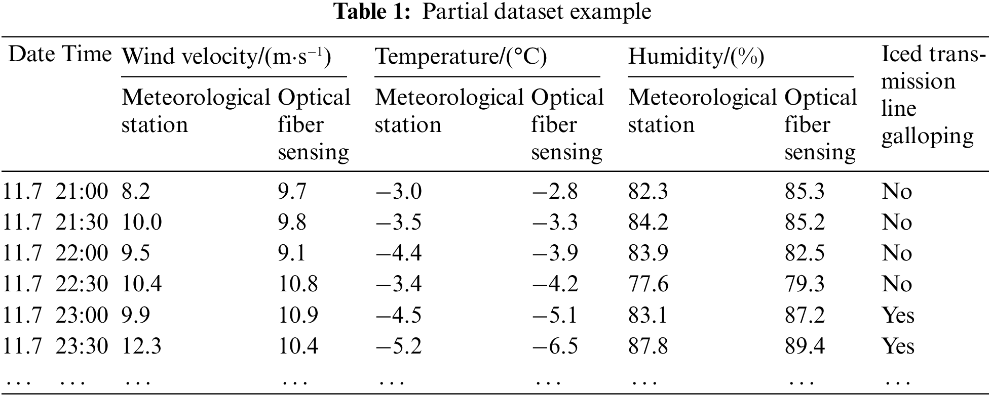
•   Multi-Dimensional Scenario Simulation Validation for Galloping Early Warning Based on Realistic Dataset: By collecting a vast amount of realistic data from iced transmission line galloping, a comprehensive dataset is established. Each data point includes input factors such as temperature, humidity, and wind velocity data obtained from optical fiber monitoring and meteorological stations, with output factors including manually determined galloping conditions. Utilizing this realistic dataset, multi-dimensional scenarios are constructed to simulate and validate multiple indices, including environmental data prediction accuracy, galloping risk coefficient errors, early warning accuracy, miss rates, and false alarm rates. Scenario 1 simulates the prediction errors of galloping under various data sources and clustering parameters to determine the optimal number of clusters for each parameter. These optimal parameters are then inputted into Scenario 2, where the network is trained and learned using the realistic dataset and optimal parameters, thereby enhancing the accuracy of the galloping early warning simulation validation.

2  Multi-Source Time Series Data Fusion and Clustering

Transmission line galloping often relies on single time series data sources like optical fiber sensing or weather forecast, which may not accurately reflect the actual galloping state and potential risks of the lines [11,24]. The principle of multi-source time series data fusion and clustering is shown in Fig. 1. Fusion and clustering of multi-source time series data related to transmission line galloping can significantly enhance the monitoring and early warning capabilities of transmission lines. Multi-source time series data for transmission lines include weather forecast data and optical fiber sensing data. Weather forecast data reflect external environmental conditions such as temperature, humidity, and wind velocity, while optical fiber sensing data also capture the physical states of transmission lines such as temperature and humidity in real-time. By fusing and clustering these multi-source time series data, it is possible to better capture the nonlinear relationships within the data, uncover characteristics that vary over time, identify potential line anomalies, and achieve more precise early warnings of galloping on iced transmission lines.

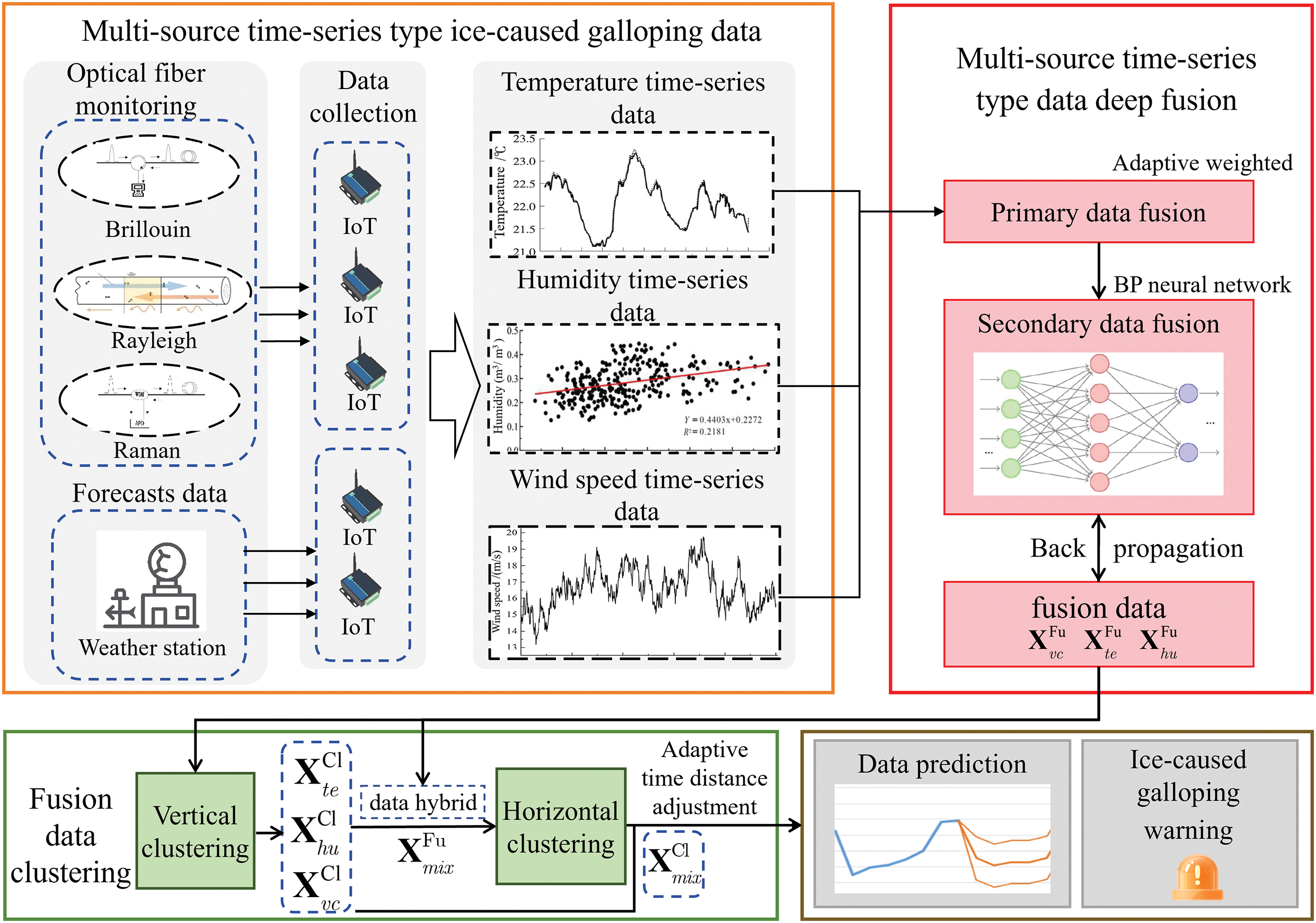
Figure 1: Multi-source time series data fusion and clustering

2.1 Deep Fusion of Multi-Source Time Series Data Based on Adaptive Weighted Learning

Through the adaptive weighted fusion of IoT driven real-time optical fiber sensing data and weather forecast data, precise assessments of the galloping state on iced transmission lines can be achieved. This section introduces a method for deep fusion of multi-source time series data based on adaptive weighted learning, providing a foundation for early warning of transmission line galloping. Initially, multi-source time series data such as temperature, humidity, and wind velocity collected by IoT driven optical fiber monitoring devices and ground meteorological stations are fused using primary adaptive weighting, with the criterion of minimizing mean square error to synthesize global environmental information at each sampling time of the transmission line. On this basis, to enhance the temporal relationships of the fused data, time series information is further extracted using a BP neural network, thus improving the quality of the fused data.

(1) Primary Data Fusion Based on Adaptive Weighting

Data types related to galloping on iced transmission lines and sensed by optical fiber sensors include temperature, humidity, and wind velocity. Taking temperature data of the transmission line as an example, suppose there are N optical fiber temperature sensors along the transmission line, each sensor collects temperature data at a fixed time interval τ. Similarly, suppose there are M ground meteorological stations that predict the temperature of the transmission line at the same interval, resulting in M sets of weather forecast data. The multi-source temperature dataset at the t-th sampling time, which combines optical fiber sensing and weather forecast, is represented as

Xte(t)={Xte,1(t),⋯,Xte,i(t),⋯,Xte,N(t),⋯,Xte,N+M(t)}(1)

where Xte,i(t),i=1,2,⋯,N represents the temperature data sensed by the i-th optical fiber temperature sensor at the t-th sampling time, providing an unbiased estimate of the true temperature Xtereal(t), with sensing errors due to equipment aging. Each measurement is independent. Xte,i(t),i=N+1,N+2,⋯,N+M corresponds to the temperature prediction data from the i-th ground meteorological station, offering a biased estimate of the true temperature Xtereal(t), with each prediction also being independent. The variances of the temperature data errors relative to their true values are denoted by δte,12,⋯,δte,N2,δte,N+12,⋯,δte,N+M2. Therefore, the total mean square error of the temperature data at time t is represented as

δte2(t)=E[(x−x^)2]=E[∑i=1N+Mwi(Xte(t)−Xte,i(t))2]=∑i=1N+Mwiδte,i2(2)

where w1,⋯,wN,wN+1,⋯,wN+M represents the adaptive weighting coefficients for each optical fiber sensing data and weather forecast data, and it is established that ∑i=1N+Mwi=1. δte2(t) is a multivariate quadratic function of these adaptive weights. According to the principle of extremum determination for multivariate functions, the minimum mean square error is achieved when δte2(t)=1/∑i=1N+M1δte,i, which represents the lower bound of the error.

The primary fusion process of adaptive weighted multi-source time series data maximizes the inherent correlations among the temperature data sensed by different sensors. The fusion result, which minimizes the mean square error, serves as the final outcome for the multi-dimensional temperature data fusion. The adaptive weighted primary fusion results of the optical fiber sensing data and weather forecast data at the t-th sampling instance can be expressed as

Xtefu(t)=∑i=1N+MwiXte,i(t),i=1,…,N,N+1,…,N+M(3)

Following the aforementioned steps, the fused time series dataset of transmission line temperatures can be obtained as Xtefu={Xtefu(1),Xtefu(2),⋯,Xtefu(T)}. Similarly, the adaptive weighted primary fusion time series sequences for humidity and wind velocity data can be obtained as Xhufu={Xhufu(1),Xhufu(2),⋯,Xhufu(T)} and Xvcfu={Xvcfu(1),Xvcfu(2),⋯,Xvcfu(T)}.

(2) Secondary Data Fusion Based on BP Neural Network

While the primary adaptive weighted fusion of multi-source optical fiber sensing data and weather forecast data can enhance the accuracy of early galloping warnings, the temporal and spatial differences between fiber optic sensors and ground meteorological stations mean that adapting weights based on sampling instances may not fully preserve the temporal characteristics of the galloping data. Therefore, this section proposes a secondary data fusion method based on the BP neural network. The temperature, humidity, and wind velocity data from the transmission lines, fused via adaptive weighting, are used as input to the BP neural network to learn and capture latent temporal patterns. The output is the secondary fused data at each sampling instance, effectively reducing data noise and irregularities. Taking the primary fusion time series sequence of temperature Xtefu as an example, the dataset is divided into a training set and a test set at a ratio of 3:1, and the steps to train the secondary data fusion BP neural network are as follows:

Step 1: Initialize network weights ϖte and bias b;

Step 2: Input the temperature time series sequence Xtefu, derived from primary adaptive weighted fusion, as the training sample for forward network training;

Step 3: Compute the loss function as

LFu=1t∑q=1|XteFu|∑p=1t(Xte,qFu(p)−X^te,qFu(p))2(4)

where |XteFu| is the number of fused time series samples, X^te,qFu(p) represents the fused value, and Xte,qFu(p) is the actual value, which is obtained through field measurements. The loss function LFu is used to assess the error in the secondary data fusion by the BP neural network, facilitating subsequent network training.

Step 4: Based on the loss function, perform back propagation using gradient descent to update the network parameters.

Step 5: Re-input the results obtained from the primary fusion into the trained secondary data fusion BP neural network to achieve the final secondary fusion results.

Based on the above steps, the secondary fusion data for temperature, humidity, and wind velocity can be obtained as XteFu={XteFu(1),XteFu(2),⋯,XteFu(T)}, XhuFu={XhuFu(1),XhuFu(2),⋯,XhuFu(T)}, and XvcFu={XvcFu(1),XvcFu(2),⋯,XvcFu(T)}.

2.2 Galloping Fusion Data Clustering Processing of Iced Transmission Lines Based on K-Medoids

After obtaining the fused data, due to the complexity and strong non-linearity of optical fiber sensing data and weather forecast data, direct prediction of the fused data can lead to non-convergence of the neural network, thereby affecting the accuracy of data predictions. Therefore, the K-Medoids algorithm is employed to cluster the high-dimensional fused data, effectively reducing data redundancy and better mining the nonlinear features of the galloping data on iced transmission lines. Clustering includes vertical clustering analysis of the data itself and horizontal clustering analysis of various fused data. Vertical clustering, by analyzing the correlations within the fused data, identifies typical patterns of variation over different time periods, thereby revealing the periodicity and anomalies of data, and enhancing data interpretability and the accuracy of prediction models. Horizontal clustering combines various fused data for a comprehensive analysis. This approach reveals the complex interactions and correlations between different data sequences. It helps to identify multidimensional interaction patterns and potential causal relationships, thus enhancing the understanding and prediction of the risks associated with galloping on iced transmission lines.

K-medoids, an improvement over K-means, select the mean of data samples as the cluster center point. Choosing actual data points from the fused data samples as cluster centers, it can mitigate the impact of outlier values during clustering, thereby addressing the issue of clustering results falling into local optima. The steps of the K-medoids clustering method include initializing cluster centers, clustering into clusters, updating the cluster center point, and convergence judgment. Taking the temperature fusion data XteFu as an example, the steps are described as follows:

Step 1: Initialize the cluster centers by randomly selecting Kte temperature fusion data samples from the transmission line as the initial set of center points for vertical clustering.

Step 2: Sequentially calculate the Euclidean distance from all data points in the fused dataset to each vertical cluster center point, and assign each data point to the cluster whose center point is closest. The calculation of the Euclidean distance is given by

Δ(kte)=∑i=1t(XteFu(i)−XteFu(kte))2(5)

where kte is an initial randomly selected cluster center point, and XteFu(i) represents the value of the temperature fusion data at the i-th sample point.

Step 3: After completing the vertical clustering, select each sample point within each cluster to serve as a new center for vertical clustering. Recalculate the Euclidean distances and select the sample point that minimizes the total distance within the cluster, designating this point as the new center of the cluster, represented as

ktenew=argminXteFu(i)∈kte∑XteFu(j)∈kte∥XteFu(i)−XteFu(j)∥2(6)

where XteFu(i) and XteFu(j) are the sample points in the cluster, and kte is the vertical clustering center.

Step 4: When the set of vertical cluster centers remains unchanged, the algorithm terminates and outputs the final vertical clustering result as XteCl={XteFu(1),⋯,XteFu(ktel),⋯,XteFu(Kte)}, where XteFu(ktel) is the dataset of the ktel-th cluster in the vertical fusion of temperature data. Otherwise, update the cluster centers and repeat Steps 2 to 4 until the set of cluster centers stabilizes.

Using the described method, the vertical clustering results for humidity and wind velocity are obtained as XhuCl={XhuFu(1),⋯,XhuFu(ktel),⋯,XhuFu(Khu)} and XvcCl={XvcFu(1),⋯,XvcFu(ktel),⋯,XvcFu(Kvc)}, where Khu and Kvc are the numbers of clusters for the vertical clustering of humidity fusion data and wind velocity fusion data, respectively. Furthermore, to analyze the relationships among different types of data, the three types of fused data are horizontally mixed. The horizontal data format for a single sample point in the mixed fused data is represented as XmixFu(t)=ωteXteFu(t)+ωhuXhuFu(t)+ωvcXvcFu(t)}, where ωte, ωhu, and ωvc are the normalized weights for the corresponding fused data. The results of the horizontal clustering of the mixed fused data are expressed as XmixCl={XmixFu(1),⋯,XmixFu(ktel),⋯,XmixFu(Kmix)}, where Kmix is the number of clusters for the mixed fused data.

2.3 Irregular Time Series Analysis of Multi-Source Data

The principle of irregular time series in multi-source data is shown in Fig. 2. The time interval of time series data is defined as the time difference between traditional adjacent sensing points, and the time distance is defined as the time difference between historical sensing points and prediction points. Typically, time-series data such as temperature, humidity, and wind velocity are collected at fixed time intervals. For instance, temperature fusion data have regular time interval [XteFu(t)−XteFu(t−1)]=[XteFu(t−1)−XteFu(t−2)]=τ and regular time distance d={d(t)=τ,d(t−1)=2τ,⋯,d(t−n)=[t+1−n]τ}. Such regularity allows time series neural networks to effectively learn these temporal patterns and achieve prediction outcomes. However, after data clustering, the data points within each subclass are no longer temporally continuous, and their intervals become irregular, leading to issues of irregular time distance. On one hand, after clustering similar data, the time distance within each data subset changes irregularly, causing vertical irregularities in time series among similar data subsets. On the other hand, after clustering the fused data, the time distance of each fused data subset changes irregularly, resulting in horizontal irregularities in time series. For example, the vertical irregular time distance for temperature data can be represented as d={d(t)=τ+N1τ,d(t−1)=2τ+N1τ,⋯,d(t−n)=[t+1−n]τ+Nnτ}, leading to irregular time series. Directly inputting these clustered subset data into a time series neural network for training makes it difficult to capture the temporal patterns, resulting in convergence performance degradation.

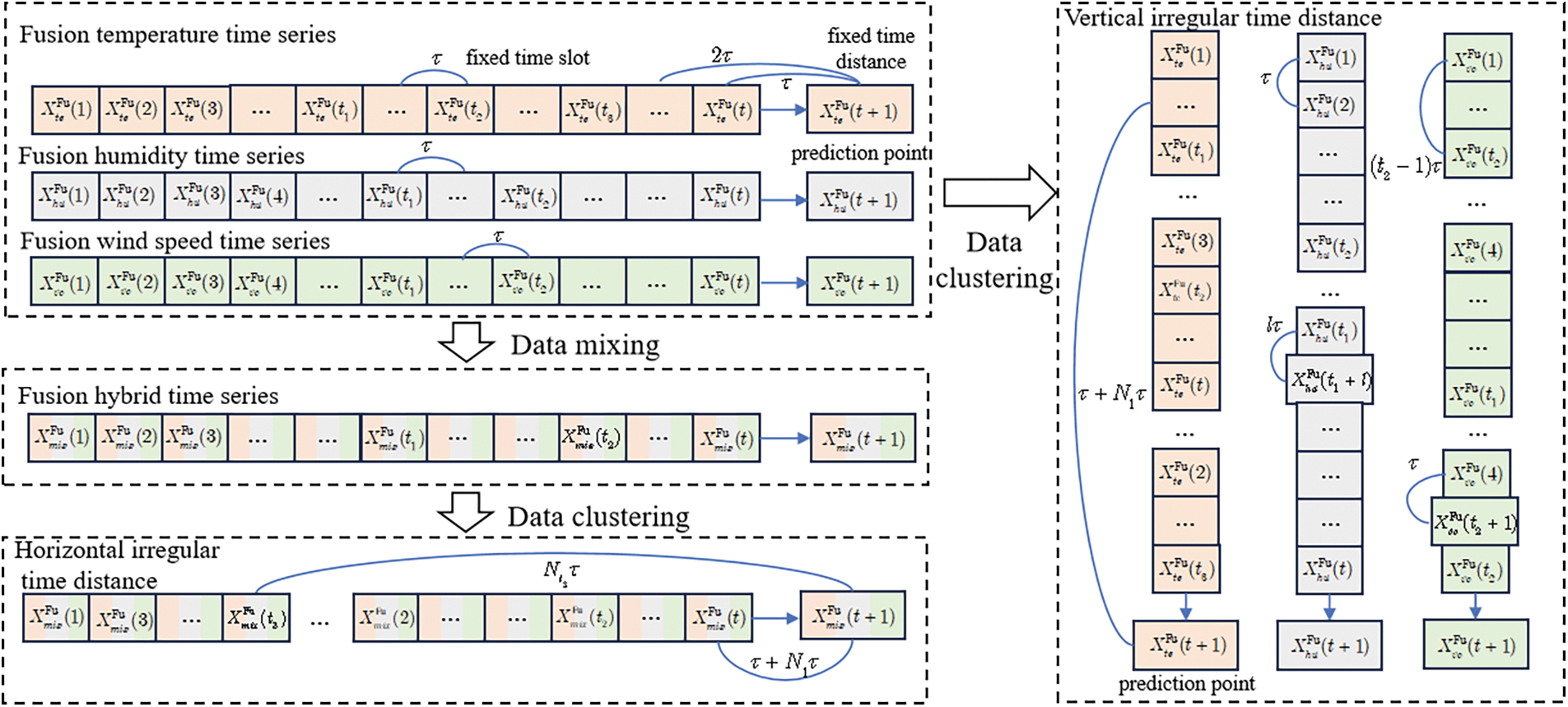
Figure 2: Irregular time series of multi-source data

3  Early Warning Algorithm for Iced Transmission Line Galloping Based on Irregular Time Series Perception and Closed-Loop Attention Mechanism

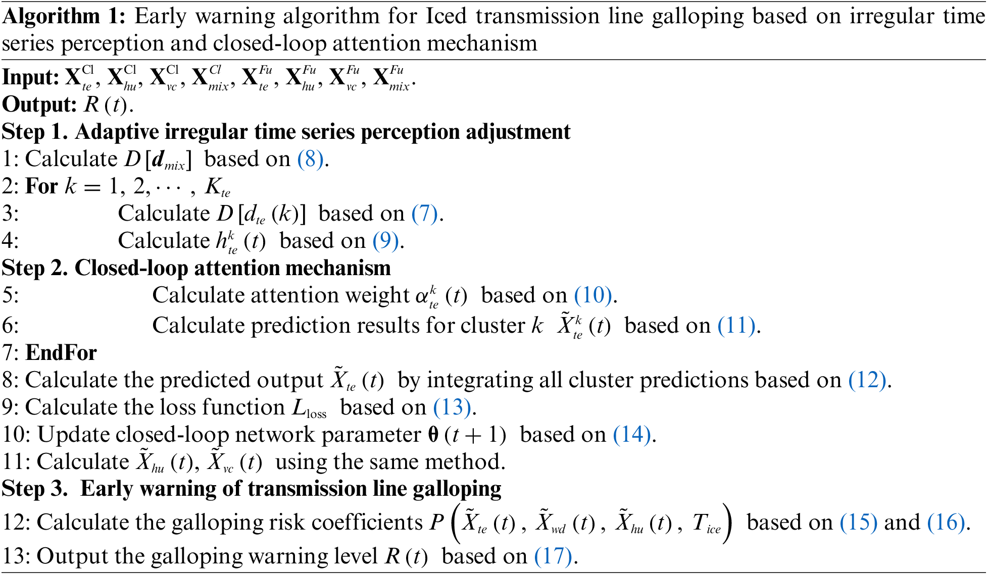
To address the issue of irregular time series in multi-source data from the clustering process, we present an early warning algorithm for iced transmission line galloping based on irregular time series perception and closed-loop attention mechanism. The principle of the algorithm is illustrated in Fig. 3. The GRU algorithm was used in this paper to predict galloping motion data. GRU is a variant of recurrent neural networks, capable of effectively handling sequential data and is a type of deep learning algorithm. Deep learning is a method of machine learning that aims to mimic the way the human brain processes information by constructing multi-layered neural networks. It extracts high-level features from input data through multiple layers of nonlinear transformations. Initially, multiple GRU networks, which are sensitive to irregular time series, predict temperature, humidity, wind velocity, and fused data separately. These networks are enhanced with an attention mechanism to refine traditional GRU network predictions, calculate risk values, and output warning results. Finally, the loss function is calculated based on the comparison between the final prediction outcomes and actual values, facilitating closed-loop training for attention and GRU network parameters. The specific flow of the algorithm is shown in Algorithm 1.

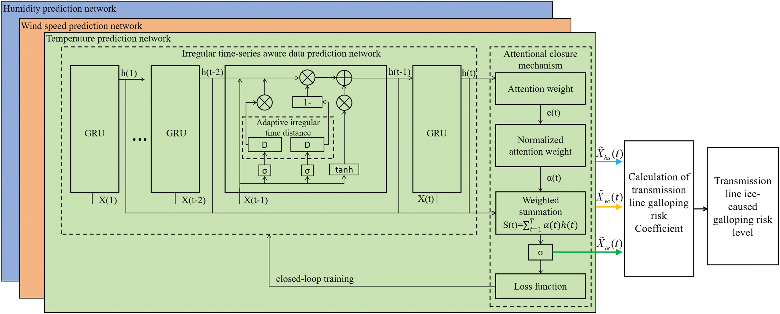
Figure 3: Early warning algorithm for iced transmission line galloping based on irregular time series perception and closed-loop attention mechanism

3.1 Irregular Time Series Perception Based Data Prediction Network

3.1.1 Irregular Time Series Perception Based Adaptive Adjustment

To address the issue of vertical irregular time series in similar fused data, taking multi-source temperature data fusion as an example. We propose a method for adaptive adjustment of vertical irregular time series distance, represented as

D[dte(k)]=αte−exp⁡[−βte×dte(k)]αte+exp⁡[−εte×dte(k)](7)

where αte, βte, and εte denote the parameters for adaptive irregular time series perception in temperature data, which together determine the construction of the time distance function and can adaptively adjust the time distance function based on data from different subsets. dte(k) represents the original time distance before adjustment for the k-th subclass in the temperature clustering results. Considering the irregular time series issues of different data sources, we further implement adaptive adjustment of horizontal irregular time series distance using mixed data clustering of temperature, wind velocity, and humidity, represented as

D[dmix]=1Kmix∑k=1Kmixαmix(k)−exp⁡[−βmix(k)×dmix(k)]αmix(k)+exp⁡[−εmix(k)×dmix(k)](8)

where αmix, βmix, and εmix represent the parameters for horizontal adaptive irregular time series perception. dmix={dmix(1),dmix(2),⋯,dmix(k),⋯,dmix(Kmix)} is the set of horizontal irregular time distance; dmix(k) indicates the time distance before adjustment for the k-th subclass in the mixed data clustering results.

3.1.2 Data Prediction Network Based on Closed-Loop Attention Mechanism

We improve the traditional GRU gate structure by enabling the update gate and reset gate to adaptively learn from irregular time distance information [25–27]. The enhanced time series perception function is integrated with the traditional GRU structure to update the gate structures as

{ztek(t)=D[dte(k−1)]D[dmix]σ(wtez×[xtek(t),htek(t−1)])rtek(t)=D[dte(k)]D[dmix]σ(wter×[xtek(t),htek(t−1)])Htek(t)=tanh⁡(wteH×[xtek(t),rtek(t),htek(t−1)])htek(t)=[1−ztek(t)]×htek(t−1)+ztek(t)×Htek(t)(9)

where xtek(t) represents the current input unit after interactive updating; htek(t−1) is the output from the hidden layer after interactive updating; ztek(t) is the update gate unit that incorporates time distance information; rtek(t) is the reset gate unit that incorporates time distance information; Htek(t) is the summation of the input and past hidden layer states; htek(t) is the output state of the hidden layer; wtez, wter, wteH are the weight parameters.

To rapidly filter out important information from a large volume of data and further enhance the temporal capture capability of the irregular time series perception based data prediction network, we use the attention mechanism to swiftly filter a large amount of information by assigning different weights to the outputs of the hidden layer, thereby strengthening the impact of important information. The attention weights are represented as

{etek(t)=uteetanh⁡[wteehtek(t)+btee]αtek(t)=softmax[etek(t)](10)

where etek(t) is the attention probability distribution, αtek(t) is the normalized attention probability distribution, utee, btee, and wtee are the attention weight parameters. The hidden layer output corrected by the attention weights and the final prediction output are given by

{Stek(t)=∑t=1Tαtek(t)htek(t)X~tek(t)=σ(wteoStek(t)+bteo)(11)

where Stek(t) is the attention-corrected hidden layer output; X~tek(t) is the prediction output at time t+1 based on clustering result k; wteo and bteo are the output weight parameters. Considering the prediction data of all clustering results, the final prediction output is expressed as

X~te(t+1)=1Kte∑k=1KteωtekX~tek(t)(12)

where ωtek is the prediction weight for the temperature clustering result k.

The goal of the irregular time series perception based data prediction network is to minimize the error between the predicted data and the actual data. We combine mean absolute error and root mean square error to train the irregular time series perception based data prediction network. The gradient of the loss function is used to update the model parameters, thereby gradually reducing the loss function and improving the accuracy of the model’s early warning predictions. The loss function and closed-loop attention training method are expressed as

Lloss=αMAET∑t=1T|Xte(t)−X~te(t)|+αRMSE1T∑t=1T(Xte(t)−X~te(t))2(13)

θ(t+1)=θ(t)−ρ∇θLloss(14)

where θ(t)={utee,wtee,btee,wteo,bteo,wtez,wter,wteH} are the network parameters, and ρ is the learning rate. The prediction method and network training method for wind velocity and humidity data are the same as those for the temperature irregular time series perception based data prediction network described above.

3.2 Transmission Line Galloping Early Warning Based on Prediction Data and Galloping Risk Coefficient

Based on the aforementioned irregular time series perception based data prediction network, the prediction datasets for temperature, humidity, and wind velocity can be obtained, represented as

{X~te={X~te(T+1),X~te(T+2),⋯,X~te(T+N)}X~hu={X~hu(T+1),X~hu(T+2),⋯,X~hu(T+N)}X~vc={X~vc(T+1),X~vc(T+2),⋯,X~vc(T+N)}(15)

Iced transmission line galloping is a process where environmental temperature, relative humidity, and wind velocity collectively accumulate energy, eventually causing the line to gallop. When analyzing the factors affecting galloping, besides the meteorological parameters such as temperature and humidity at specific times, physical quantities representing the accumulation process, such as duration, should also be considered. The four parameters that have the greatest impact on transmission line galloping under icing conditions are temperature, wind velocity, humidity, and icing duration. The transmission line galloping risk coefficient is expressed as

P(X~te(t),X~wd(t),X~hu(t),Tice)=∑t∈Ticek⋅f(t)⋅X~teα(t)⋅X~wdβ(t)⋅X~huγ(t)(16)

where X~te(t), X~wd(t), and X~hu(t) represent the predicted values of temperature, wind velocity, and humidity at time t, respectively. Tice is the icing duration, k is the icing galloping intensity coefficient, and f(t) is the unit time galloping risk factor. The galloping of the transmission line under icing conditions requires sustained meteorological factors to generate energy accumulation, and the unit time galloping risk factor decreases over time. According to statistical principles, the unit time galloping risk factor can be expressed as

f(t)=1−122π∫te−(τ−6)28dτ(17)

Substituting (17) into (16), the transmission line galloping risk coefficient can be expressed as

P(X~te(t),X~wd(t),X~hu(t),Tice)=∑t∈Tice(1−122π∫te−(τ−6)28dτ)⋅X~teα(t)⋅X~wdβ(t)⋅X~huγ(t)(18)

Further based on the principles of mathematical statistics and actual data of iced transmission line galloping, the galloping risk coefficients of different galloping events are classified to derive the transmission line icing galloping risk levels characterized by the galloping risk coefficient, expressed as

R(t)={Level IVP(X~te(t),X~wd(t),X~hu(t),Tice)>0.9Level III0.8<P(X~te(t),X~wd(t),X~hu(t),Tice)⩽0.9Level II0.6<P(X~te(t),X~wd(t),X~hu(t),Tice)⩽0.8LevelI0.4<P(X~te(t),X~wd(t),X~hu(t),Tice)⩽0.6(19)

4  Simulation

To verify the effectiveness of the proposed method, we employ a realistic historical dataset from a transmission line for case verification. The dataset contains historical data spanning several months, with the minimum time interval between each raw data point being 5 min. The dataset comprises 20,000 samples, with each sample point including input factors such as temperature, humidity, and wind velocity data obtained through optical fiber sensing and meteorological stations, and output factors including manually determined galloping conditions. The dataset is shown in Table 1. The first 15,000 samples are used as the training set, and the remaining 5000 samples are used as the test set. The training set data and results are used to train the irregular time series perception based data prediction network. The meteorological data from the test set are input into the trained network for data prediction and galloping early warning. According to (18), the predicted data are compared with the actual monitoring data, and the early warning results are compared with the actual records to verify the effectiveness of the proposed method. Multi-dimensional simulation scenarios are constructed, where Scenario 1 is used for the analysis of data clustering and fusion results, and Scenario 2 is used for the analysis of prediction results and early warning results.

In addition, to verify the effectiveness of the proposed irregular time series perception based data prediction network, two comparison algorithms are selected for analysis. Baseline 1 uses the traditional GRU algorithm without data clustering fusion and irregular time series perception adjustment [27]. Baseline 2 uses the LSTM algorithm with data clustering but without irregular time series perception adjustment [28]. The comparison algorithms use the same training set and test set as the proposed algorithm for simulation. By comparing data prediction accuracy and algorithm convergence speed, the performance of the proposed algorithm is verified.

4.1 Data Clustering and Fusion Results Analysis

Fig. 4 illustrates the clustering results using temperature data as an example. As seen in the figure, the number of samples in each subset after clustering is 1908, 2297, 5523, 4915, 3014, and 2343, respectively. The histogram further illustrates that the average time intervals between different subsets vary, with mean values of 28, 23, 6, 9, 19, and 22 steps, respectively, and an overall average of 17.83 steps. It is evident that subsets with fewer sample points tend to have longer time intervals. In practical applications, if the data within a subset is too sparse after clustering, the number of clusters can be appropriately reduced. The results in the figure reflect the irregular time distance generated by the clustering algorithm, laying the foundation for subsequent adaptive irregular time series perception adjustment.

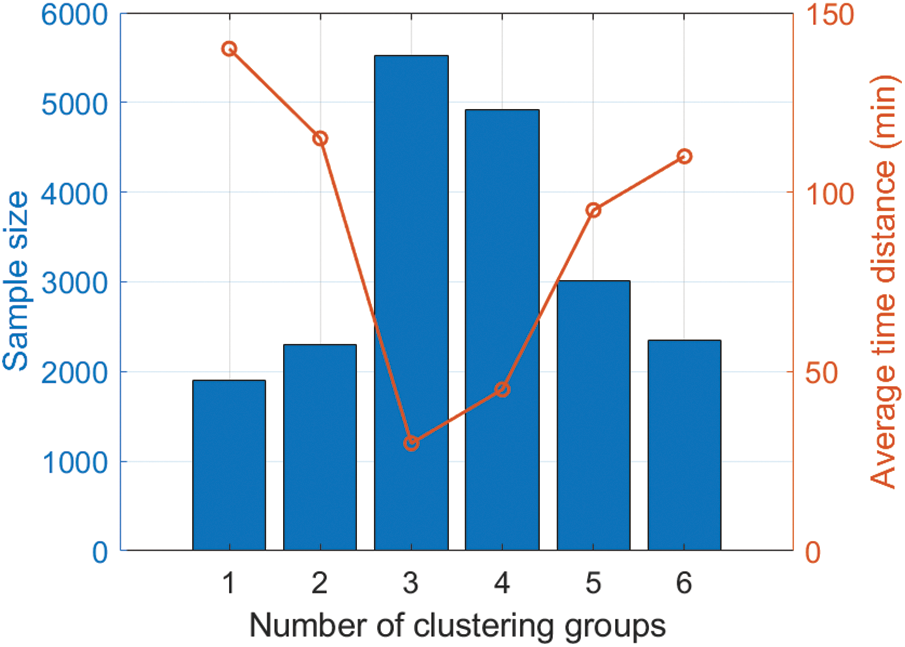
Figure 4: The clustering results using temperature data

Fig. 5 illustrates the meteorological data prediction errors under different data sources and clustering parameters using the proposed algorithm. When using fused data from both meteorological stations and optical fiber sensing, the average prediction error decreases by 32.4% and 12.9%, respectively, compared to using each data source independently. This improvement is due to the better capture of nonlinear relationships within multi-source time series data through fusion and clustering, resulting in more accurate predictions. For different data sources, the number of clusters significantly affects prediction accuracy. The figure indicates that the minimum prediction error occurs with 5, 5, and 6 clusters for the three data sources, respectively. This is because the data characteristics become more complex after fusion, and more clusters can better capture the potential correlations within the data, enhancing prediction accuracy. However, when the number of clusters continues to increase, prediction error grows rapidly due to the separation of correlated features, reducing the temporal correlation within similar data, and leading to decreased prediction accuracy.

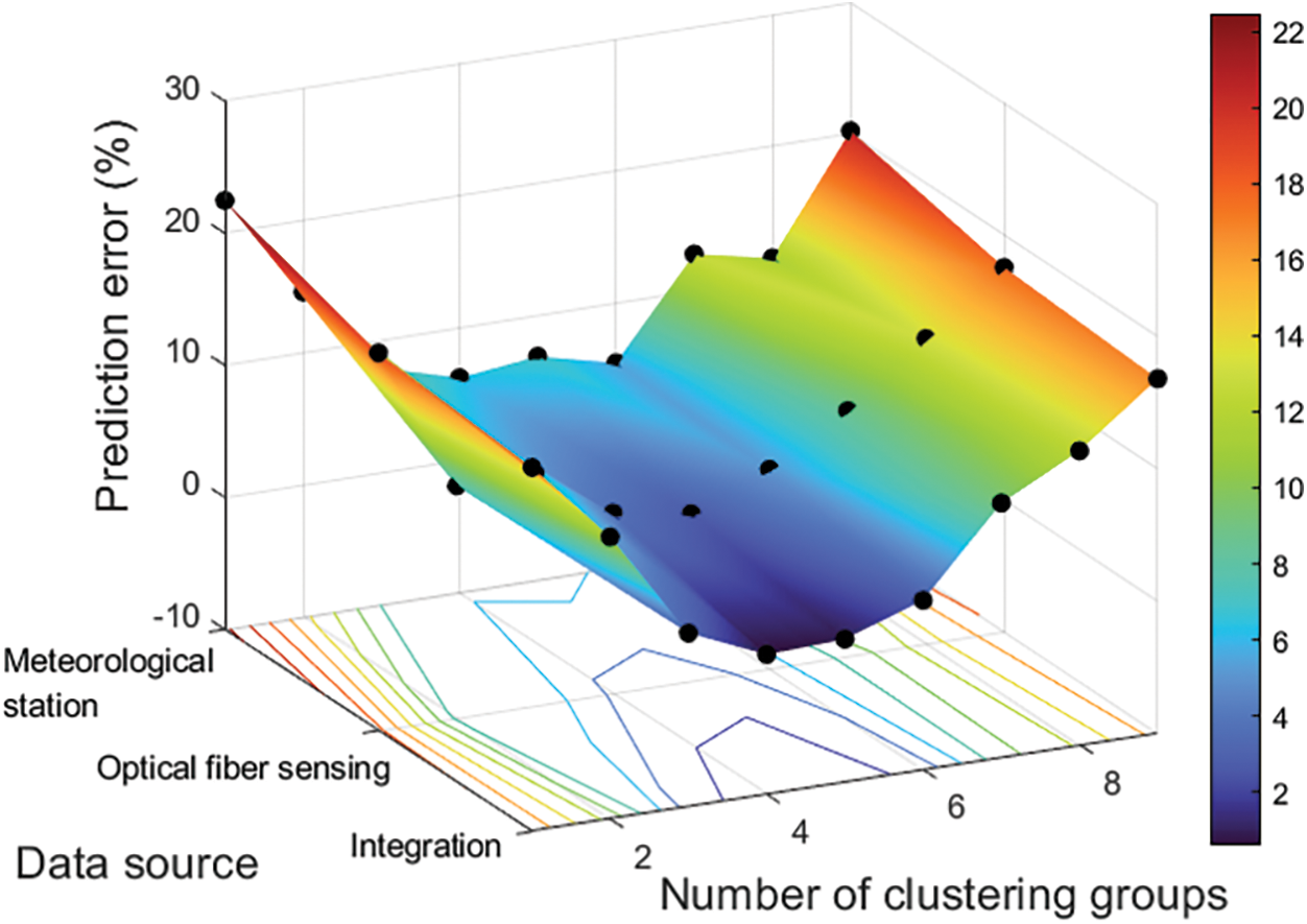
Figure 5: The meteorological data prediction errors under different data sources and clustering parameters using the proposed algorithm

4.2 Data Prediction Performance Analysis

Figs. 6–8 respectively illustrate the prediction results of temperature, wind velocity, and humidity for the time period from 17:00 to 23:00 using the proposed algorithm. The figures indicate that the prediction errors for the three data types are reduced by 69.47% and 14.13%, 55.25% and 22.44%, and 72.48% and 28.29% compared to the two comparison algorithms, respectively. This is because the proposed algorithm first performs a secondary deep fusion of multi-source time series data, which better captures the nonlinear relationships within the data. Secondly, the proposed algorithm performs horizontal and vertical clustering on the fused data to improve data correlation and constructs an adaptive time series perception adjustment module to address the issue of irregular time series in the clustered data, ensuring the algorithm’s ability to perceive and predict irregular time series data. Furthermore, the proposed algorithm introduces a closed-loop attention mechanism into the traditional GRU network structure, enhancing the algorithm’s ability to filter important information, and strengthening the learning capability through closed-loop updates, ultimately improving the prediction accuracy of the proposed algorithm.

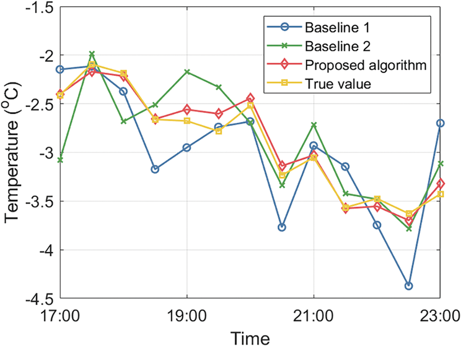
Figure 6: The prediction results of temperature vs. time

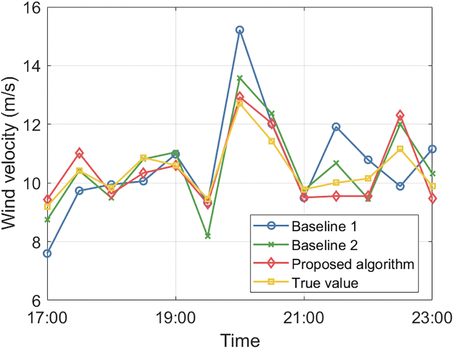
Figure 7: The prediction results of wind velocity vs. time

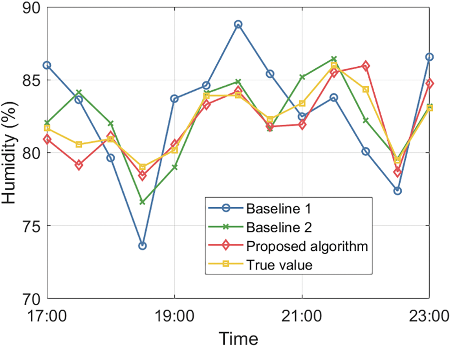
Figure 8: The prediction results of humidity vs. time

Fig. 9 illustrates the comparison of the loss function value reduction process vs. iterations. The figure demonstrates that after 200 iterations, the loss function value of the proposed algorithm is reduced by 47.98% and 38.82% compared to Baseline 1 and Baseline 2, respectively. This improvement is due to the proposed algorithm’s consideration of irregular time series perception during model training, addressing the irregular time series issue in multi-source data, thereby increasing the algorithm’s convergence speed. Additionally, the proposed algorithm improves the gate structure of the traditional GRU network, enabling the update and reset gates to adaptively learn from irregular time distance information, thus enhancing the network’s data prediction accuracy.

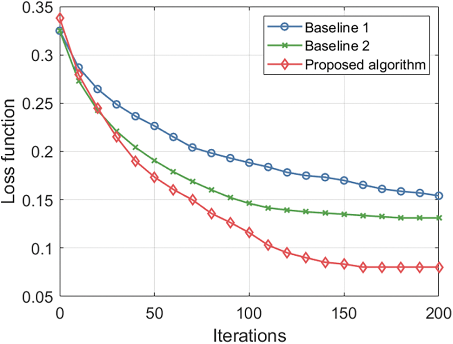
Figure 9: The comparison of the loss function value reduction process vs. iterations

4.3 Early Warning Effectiveness Analysis

Fig. 10 illustrates the relative error in calculating the galloping risk coefficient for 80 randomly selected sample points using different algorithms, where the true values are obtained from actual meteorological data. The figure indicates that the average error in the galloping risk coefficient calculated by the proposed algorithm is reduced by 67.1% and 59.4% compared to the comparison algorithms. This improvement is due to the deep fusion as well as horizontal and vertical clustering of multi-source raw data by the proposed algorithm, which significantly enhances the correlation of the original data and deeply mines the temporal characteristics of the data, laying a foundation for subsequent data prediction. Additionally, the proposed algorithm constructs an attention closed-loop mechanism that can backpropagate to adjust network parameters based on the final prediction error, enhancing the learning ability of the algorithm and ensuring the accuracy of meteorological prediction data. With more accurate prediction data, the final calculation of the galloping risk coefficient by the proposed algorithm is more precise. The relevant simulation results are shown in Fig. 11 and Table 2.

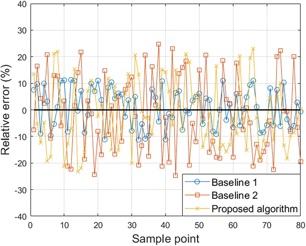
Figure 10: The relative error in calculating the galloping risk coefficient using different algorithms

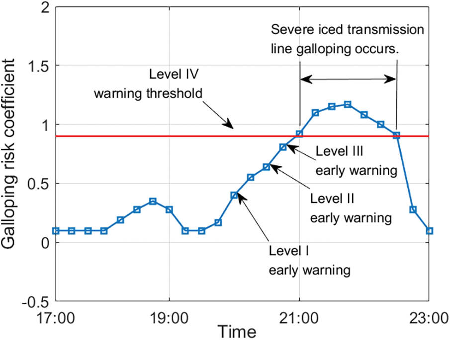
Figure 11: The early warning process of the proposed algorithm before and after an iced transmission line galloping event

Fig. 11 illustrates the early warning process of the proposed algorithm before and after an iced transmission line galloping event in the dataset. The figure shows that the proposed algorithm issues Levels I, II, and III warnings respectively before the galloping event, providing early warnings up to 4 h in advance, thus ensuring ample time for emergency response. This is because the proposed algorithm constructs an adaptive time series perception adjustment module, enabling the neural network to adjust for irregular time series. Additionally, the introduction of the attention closed-loop mechanism enhances the network’s ability to filter and learn important information, ensuring the accuracy of the prediction data, and thereby providing data support for galloping early warning. Furthermore, the proposed algorithm calculates the galloping risk coefficient using the unit time impact factor, perceiving energy accumulation during iced transmission line galloping, thereby increasing the sensitivity to time series data and achieving precise early warnings for icing galloping.

The early warning results of the proposed algorithm for the test set data of iced transmission line galloping are shown in Table 2. The missed alarm rate of the proposed algorithm is reduced by 71.07% and 63.52%, respectively, compared to the comparison algorithms, and the false alarm rate is reduced by 42.71% and 46.58%. This improvement is due to the proposed algorithm’s comprehensive consideration of data fusion, adaptive irregular time series perception adjustment, and attention closed-loop mechanisms, enhancing the perception and prediction capabilities for time series data. The proposed meteorological data prediction network achieves accurate meteorological data predictions, providing a data foundation for subsequent galloping early warning. The reasons for false alarms in the proposed algorithm are as follows: 1. The proposed model is highly sensitive to future line galloping, which may result in early warning signals, and such false alarms can still provide early warning function; 2. The dataset’s galloping conditions are manually labeled, which may result in missed labels where small-scale galloping events occurred but were not observed manually. The low missed alarm rate of the proposed algorithm ensures comprehensive early warnings for transmission line galloping, achieving the purpose of early warning and prevention in actual application.

5  Conclusion

In this paper, we proposed an early warning method of transmission line galloping based on the integration of optical fiber sensing and weather forecast time series data. First, multi-source time series data were deeply fused based on adaptive weighted learning, and K-mediods were used to cluster the fused data of iced transmission line galloping. Next, the traditional iced transmission line galloping data prediction network was improved through adaptive adjustment of irregular time series perception and attention to closed-loop mechanism, comprehensively considering the effects of temperature, humidity, wind velocity, and duration to construct an iced transmission line galloping risk coefficient, and early warnings were issued based on the risk coefficient. Finally, using a historical dataset of transmission lines, the proposed algorithm’s performance was validated by dividing the dataset into training and test sets. The results show that, compared to the two comparison algorithms, the proposed algorithm reduces the prediction errors of temperature by 69.47% and 14.13%, the prediction errors of wind velocity by 55.25% and 22.44%, and the prediction errors of humidity by 72.48% and 28.29%. The average error of the galloping risk coefficient is reduced by 67.1% and 59.4%, the missed alarm rate is reduced by 71.07% and 63.52%, and the false alarm rate is reduced by 42.71% and 46.58%. The current research in this paper still has some limitations. For example, only the early warning of galloping is considered, and the integrated mechanism of perception and control is not established, which cannot realize the highly-reliable monitoring of icing galloping on transmission lines. In addition, this paper uses an idealized perception data model, without considering the problem of data loss caused by sensor and communication errors, which may lead to a decline in the accuracy of the final warning results in practical application. In the future, we will establish a comprehensive monitoring system for transmission lines based on machine learning, taking into account the impact of false data injection on predictive models, and introduce data encryption and identity authentication mechanisms to further improve the accuracy of transmission line icing galloping warning and the cyber security of the comprehensive monitoring system.

Acknowledgement: The authors appreciate it that this research was funded by Science and Technology Project of State Grid Corporation of China.

Funding Statement: This research was funded by Science and Technology Project of State Grid Corporation of China under grant number 5200-202319382A-2-3-XG.

Author Contributions: Conceptualization, Zhe Li, Yun Liang, and Jinyu Wang; methodology, Zhe Li, Yun Liang, Jinyu Wang and Yang Gao; formal analysis, Yun Liang and Yang Gao; investigation, Zhe Li; simulation, Zhe Li, Jinyu Wang and Yang Gao; data curation, Yun Liang and Jinyu Wang; writing—original draft preparation, Zhe Li, Yun Liang and Jinyu Wang; writing—review and editing, Zhe Li, Yun Liang, Jinyu Wang and Yang Gao. All authors reviewed the results and approved the final version of the manuscript.

Availability of Data and Materials: Data sharing is not applicable to this article as no new data were created or analyzed in this study.

Ethics Approval: Not applicable.

Conflicts of Interest: The authors declare no conflicts of interest to report regarding the present study.

References

1. Y. Liu et al., “A novel foreign object detection method in transmission lines based on improved YOLOv8n,” Comput. Mater. Contin., vol. 79, no. 1, pp. 1263–1279, Apr. 2024. doi: 10.32604/cmc.2024.048864. [Google Scholar] [CrossRef]

2. L. Yang, Y. Chen, Y. Hao, L. Li, H. Li and Z. Huang, “Detection method for equivalent ice thickness of 500-kV overhead lines based on axial tension measurement and its application,” IEEE Trans. Instrum. Meas., vol. 72, no. 4, pp. 1–11, Apr. 2023. doi: 10.1109/TIM.2023.3264035. [Google Scholar] [CrossRef]

3. L. Huang et al., “The quantitative detection system and method for natural ice covering of composite insulators by quasi-distributed fiber bragg gratings,” IEEE Trans. Power Deliv., vol. 38, no. 6, pp. 4061–4069, Dec. 2023. doi: 10.1109/TPWRD.2023.3301027. [Google Scholar] [CrossRef]

4. A. Shoukat, M. A. Mughal, S. Y. Gondal, F. Umer, T. Ejaz and A. Hussain, “Optimal parameter estimation of transmission line using chaotic initialized time-varying PSO algorithm,” Comput. Mater. Contin., vol. 71, no. 1, pp. 269–285, Jan. 2022. [Google Scholar]

5. J. Si, X. Rui, L. Bin, L. Zhou, and S. Liu, “Development of a wind spoiler anti-galloping device for bundle conductors of UHV overhead transmission lines,” IEEE Trans. Power Deliv., vol. 35, no. 3, pp. 1348–1356, Jun. 2020. doi: 10.1109/TPWRD.2019.2943383. [Google Scholar] [CrossRef]

6. W. Lou, Z. Wen, and H. Liang, “A multi-objective optimization framework for anti-galloping of UHV transmission lines using MTTMD based on weighted satisfaction,” IEEE Trans. Power Deliv., vol. 37, no. 1, pp. 249–257, Feb. 2022. doi: 10.1109/TPWRD.2021.3056094. [Google Scholar] [CrossRef]

7. B. Huo, X. Liu, and S. Yang, “Galloping of iced transmission lines considering multi-torsional modes and experimental validation on a continuous model,” IEEE Trans. Power Deliv., vol. 37, no. 4, pp. 3016–3026, Aug. 2022. doi: 10.1109/TPWRD.2021.3121269. [Google Scholar] [CrossRef]

8. Z. Zhang et al., “Vulnerability of machine learning approaches applied in IoT-based smart grid: A review,” IEEE Internet Things J., vol. 11, no. 11, pp. 18951–18975, Jun. 2024. doi: 10.1109/JIOT.2024.3349381. [Google Scholar] [CrossRef]

9. K. Sharma, A. Malik, I. Batra, A. S. M. S. Hosen, M. A. L. Sarker and D. S. Han, “Technologies behind the smart grid and internet of things: A system survey,” Comput. Mater. Contin., vol. 75, no. 3, pp. 5049–5072, Apr. 2023. doi: 10.32604/cmc.2023.035638. [Google Scholar] [CrossRef]

10. X. Zhong, X. Sun, and Y. Wu, “Double-layer-optimizing method of hybrid energy storage microgrid based on improved grey wolf optimization,” Comput. Mater. Contin., vol. 76, no. 2, pp. 1599–1619, Aug. 2023. doi: 10.32604/cmc.2023.039912. [Google Scholar] [CrossRef]

11. T. Tan et al., “Research on monitoring the transmission line tension and galloping based on FBG fitting sensor,” IEEE Trans. Instrum. Meas., vol. 71, no. 11, pp. 1–8, Nov. 2022. doi: 10.1109/TIM.2022.3216598. [Google Scholar] [CrossRef]

12. K. Ji, L. Zhang, J. Han, H. Tang, X. Ma and K. Li, “Integrated monitoring technology for tension and inclination of overhead transmission lines based on fiber bragg grating,” in 2023 3rd Int. Conf. Electr. Eng. Mechatron. Technol. (ICEEMT), Nanjing, China, 2023, pp. 81–85. [Google Scholar]

13. S. Gao, X. Zeng, J. Li, S. Feng, and Y. Chen, “Capturing energy from power transmission lines galloping and self-powered sensing of galloping state through a rotary structural electromagnetic energy harvester,” IEEE Trans. Energy Convers., vol. 38, no. 3, pp. 1855–1867, Sep. 2023. doi: 10.1109/TEC.2023.3244661. [Google Scholar] [CrossRef]

14. L. Zheng et al., “Study on forecasting method of transmission line galloping via BP neural network,” in Proc. POWERCON, Guangzhou, China, 2018, pp. 4305–4312. [Google Scholar]

15. X. Jin, X. Zhang, X. Cheng, G. Jiang, L. Masisi and W. Huang, “A physics-based and data-driven feature extraction model for blades icing detection of wind turbines,” IEEE Sens. J., vol. 23, no. 4, pp. 3944–3954, Feb. 2023. doi: 10.1109/JSEN.2023.3234151. [Google Scholar] [CrossRef]

16. R. Jiang et al., “Intelligent fault diagnosis of hydraulic systems based on multisensor fusion and deep learning,” IEEE Trans. Instrum. Meas., vol. 73, pp. 1–15, Jul. 2024. [Google Scholar]

17. C. Liang, “Construction of soft computing anomaly detection model based on independence criteria and maximum entropy clustering algorithm,” IEEE Access, vol. 12, pp. 111111–111125, Aug. 2024. doi: 10.1109/ACCESS.2024.3440335. [Google Scholar] [CrossRef]

18. X. Zhou, N. Zhai, S. Li, and H. Shi, “Time series prediction method of industrial process with limited data based on transfer learning,” IEEE Trans. Ind. Inf., vol. 19, no. 5, pp. 6872–6882, May 2023. doi: 10.1109/TII.2022.3191980. [Google Scholar] [CrossRef]

19. Y. Wei and X. Gao, “Transmission line galloping prediction based on GA-BP-SVM combined method,” IEEE Access, vol. 9, no. 7, pp. 107680–107687, Jul. 2021. doi: 10.1109/ACCESS.2021.3100345. [Google Scholar] [CrossRef]

20. Y. Yao, M. Yang, J. Wang, and M. Xie, “Multivariate time-series prediction in industrial processes via a deep hybrid network under data uncertainty,” IEEE Trans. Ind. Inf., vol. 19, no. 2, pp. 1977–1987, Feb. 2023. doi: 10.1109/TII.2022.3198670. [Google Scholar] [CrossRef]

21. X. Wang and Y. Zhang, “Multi-step-ahead time series prediction method with stacking LSTM neural network,” in 2020 3rd Int. Conf. Artif. Intell. Big Data (ICAIBD), Chengdu, China, 2020, pp. 51–55. [Google Scholar]

22. T. Pelech-Pilichowski, “On adaptive prediction of nonstationary and inconsistent large time series data,” in 2018 41st Int. Conv. Inform. Commun. Technol., Electron. Microelectron. (MIPRO), Opatija, Croatia, 2018, pp. 1260–1265. [Google Scholar]

23. W. Wang, F. Liu, W. Wang, and M. Cheng, “The chaotic time series prediction method based on sparrow search algorithm optimization,” in 2021 2nd Int. Conf. Intell. Comput. Human-Comput. Interaction (ICHCI), Shenyang, China, 2021, pp. 104–107. [Google Scholar]

24. L. He, J. Luo, and X. Zhou, “A novel deep learning model for transmission line icing thickness prediction,” in 2021 IEEE 5th Adv. Inform. Technol., Electron. Autom. Control Conf. (IAEAC), Chongqing, China, 2021, pp. 733–738. [Google Scholar]

25. W. Chen, C. Zhai, X. Wang, J. Li, P. Lv and C. Liu, “GCN- and GRU-based intelligent model for temperature prediction of local heating surfaces,” IEEE Trans. Ind. Inf., vol. 19, no. 4, pp. 5517–5529, Apr. 2023. doi: 10.1109/TII.2022.3193414. [Google Scholar] [CrossRef]

26. C. Li, G. Tang, X. Xue, A. Saeed, and X. Hu, “Short-term wind velocity interval prediction based on ensemble GRU model,” IEEE Trans. Sustainable Energy, vol. 11, no. 3, pp. 1370–1380, Jul. 2020. doi: 10.1109/TSTE.2019.2926147. [Google Scholar] [CrossRef]

27. W. Chen, H. Zhou, L. Cheng, and M. Xia, “Wind turbine blade icing diagnosis using convolutional LSTM-GRU with improved African vultures optimization,” IEEE Open J. Instrum. Meas., vol. 1, no. 11, pp. 1–9, Nov. 2022. doi: 10.1109/OJIM.2022.3217850. [Google Scholar] [CrossRef]

28. Y. Wan, H. Hou, X. Bai, J. Lv, D. Cai and Y. Shen, “Prediction of transmission line icing thickness based on long short-term memory network,” in 2023 IEEE Int. Conf. Energy Technol. Future Grids (ETFG), Wollongong, Australia, 2023, pp. 1–6. [Google Scholar]