Assessor Feedback Mechanism for Machine Learning Model

1  Introduction

Over the last two decades, artificial intelligence (AI)-based approaches have developed many remarkable solutions, including image recognition [1], speech recognition [2], machine translation [3], sentiment analysis [4], and text and image generation [5]. Hence, the significance of the safety of deployed AI systems is boosted by the increase in the leveraging of proposed models and AI applications. If the power of AI models is not adequately assessed before deployment, it can cause remarkable undesirable events in the future [6–8].

Evaluating the robustness of AI models is challenging because researchers have encountered many issues while developing machine learning (ML). Especially deep neural network (DNN) models as adversarial examples change their outputs from the correct one to wrong [9], on image classification [10,11], on large language models [12]. Explaining these models in this phenomenon is to identify its source, which is related to either a hard instance or unknown [13]. Many conventional techniques fail when a little distribution shift occurs in the unseen data [14,15].

Traditionally, we evaluate an AI system using cross-validation (the prevailing method), which involves assessing its average performance on unseen datasets, such as accuracy in classification or mean absolute error in regression tasks on test sets. Additionally, we consider model self-confidence, which indicates the extent to which an instance aligns closely with the target. For instance, a logistic regression model generates the Maximum Class Probability (MCP), indicating the probability to which a given object belongs to either the first or second class. However, this information can be obtained only after acquiring an ML model’s output. Moreover, this represents solely the system’s certainty regarding a specific example without indicating whether the system’s prediction is accurate. As an illustration, when a DNN model classifies a perturbed image, it generates probabilities indicating the likelihood of the input image belonging to each class, following the softmax distribution [16]. However, the generated output needs to be more accurate due to its classification as an adversarial example. These methods can lead to severe accidents. For instance, if a self-driving car misidentifies a “stop sign” as a “45-km/h speed limit” due to adversarial perturbations [17].

Hence, it is essential to ascertain the accuracy of the anticipated output of any AI system prior to its deployment, at the very least by assessing the probability of success or failure for each instance. The assessor model, recently introduced by [7], is designed to evaluate AI systems in specific scenarios, determining the likelihood of success for a deployed system. This framework is underpinned by various broader impacts and illustrated with a single straightforward example of a classification problem. At its core, the model serves as an AI meta-model, overlaying deployed AI systems, and is mandated to fulfill five fundamental properties: anticipatory-forecasting the success of system outcomes for a given task before utilizing the system; autonomous-operating as a distinct model without access to internal system workings; granular-providing individual predictions for system behavior on each object; behavioral-incorporating emerging traits of deployed systems during prediction; and distributional-predicting outcomes based on system populations. Based on the characteristics, the assessor model is expected to predict the behavior of the system differently and consistently in specific scenarios. For instance, even if two systems perform the same task, they may do so in different ways, or a single system might vary its approach across situations or tasks due to varying levels of complexity.

Another method of evaluating ML models involves the application of item response theory (IRT), which gathers prediction outcomes for analysis. Unlike traditional approaches like calculating average accuracies for classification tasks, IRT pertains to the domain of psychometrics, aiming to gauge and analyze the abilities of respondents and the difficulty levels of items within a given survey. In this case, items and subjects correspond to input objects and ML models, respectively [13]. In IRT, there is done wide a range of analysis, particularly estimating the hardness of predicting each new instance by an AI system is considered [13,18]. In this paper, we also leverage responses from ML models similar to IRT to construct datasets to train and evaluate assessor models, however, the assessor-meta model learns these responses instead of computing IRT parameters to explain ML models.

In this research, we enhance the effectiveness of the assessor model by introducing a methodology aimed at reducing system errors. The initial assessor approach predicts a system’s single-input prediction’s success or failure, similar to binary classification. Therefore, if we have AI systems and their predictions on a test set, we can train an assessor model on this tuple of <system, input, systemsuccess> by assuming we have classification problems. However, this approach must be adjusted for regression problems. To implement with setting <system, input, systemsuccess>, we replace “system success” with its “error” and train the assessor model on this setting without losing any properties. Upon obtaining a prediction error from the assessor, we can determine whether to utilize the selected system based on a predefined threshold.

Our key contributions to this work: developing transformation from success probabilities to predicting errors with their inverse for continuous variables; adjusting this idea for regression, logistic regression, and classification with softmax output tasks on NN models and SVM. We also demonstrate our results in over 30 datasets to validate this proposal. Additionally, as the research focuses on ML models, the paper uses the terms “systems” or “models” interchangeably to refer to ML models, and calls the assessor model the “assessor” throughout.

The rest of the paper is organized as follows: the next section summarizes relevant work; in Section 3, we introduce the core elements of the assessor procedure, the transformation, and our proposed approach to empower it; Section 4 presents a broad range of experiments as examples of three widely used ML tasks; final sections discuss and conclude our findings.

2  Related Work

Since these assessor models have been recently proposed, their practical implementations are rare, so the following subsections present an overview of other assessing methods divided into several types. Nevertheless, one very similar approach is the use of instance hardness measure as part of the learning process [19] by subtracting the value from the output of softmax. This measurement is also computed from responses by a set of ML models, particularly multilayer perceptron, for classification tasks. Since the instance hardness is combined in the training process with backpropagation in an MLP model, the approach is not standalone.

2.1 Automated Machine Learning

Automated ML (AutoML) has been used widely to automate the entire process of building AI system pipelines, including collecting data, data preprocessing, feature engineering, feature selection, meta-learning, hyperparameter searching, and neural network architecture searching without requiring a deep knowledge of ML or any human intervention. During the hyperparameter and neural network architecture searching using meta-learning, it may use various parameters to find an appropriate model for the given task, likewise fine-tuning NN models [20,21]. Since it is so popular, many ML frameworks have developed their AutoML versions, including Autosklearn, AutoTensorflow, and AutoPyTorch. In the case of an instance-level assessment (the paper’s primary focus), we also leverage similar parameters to constitute the emergent behavior of AI systems with other related factors to this process.

The most significant difference between them is the assessor model aims to assess before employing an AI system on each task. Suppose we know how an AI system behaves for every job. In that case, we can apply this result to a range of AI problems such as combining models, explaining AI systems, fixing outputs (the main objective of this paper), and auditing or certifying [7]. Moreover, AutoML does not satisfy all properties of the assessor model listed above except distributional1.

2.2 Item Response Theory

One way to explain AI systems is to derive their IRT difficulties developed [13] supported by regression examples for a broad range of ML tasks, including adversarial examples and out-of-distribution samples. Authors acquire 10–20 responses for each item from models to estimate the difficulties by training a meta-learning model on the responses. In this case, the “difficulty estimator” model is not an assessor model that holds the above properties. Similarly, IRT responses are leveraged to build a weighted majority voting framework based on the hardness of instances in ensembles by measuring how close the objects are to the boundary [19,22]. Another analysis of AI models at the granular level based on IRT explored ML classifiers to estimate their behavior [13]. To explain these classifiers, the authors combined latent variables of items and responses by models. Most of this research has benefited from the two-parameter logistic model to identify instance abilities and difficulties as a function of probabilities as follows:

Pr(Uij=1|θj)=11+e−ai(θj−bj),

where Uij, ai, and bj are binary response of respondent i to question j, a slope, and a difficulty accordingly. These parameters facilitate explaining the model abilities and instance hardness (difficulty). Our main aim in this work is to train the assessor model to fix models’ outputs. However, we also used similar responses to construct a dataset to train the assessor model on it. These approaches also do not complete the properties of the assessor. Other work has been proposed to evaluate robustness testing of ML families [18], speech synthesis [23].

2.3 Practical Implementations of Assessors

Several recommended fields of assessors are listed in a previous study [7] along with the proposal of the assessor and its properties, providing a simple classification example to demonstrate its ability. Moreover, one study proposed selecting and combining several systems to improve performance [24]. They developed a small random forest model to estimate how large language models can compile an input prompt properly. To construct the relationship between items and responses, they extract instance features from text and use the number of shots in training with systems’ characteristics as three-dimensional space. Instead, we build this relationship differently because we aim to reduce models’ errors.

2.4 Failure Predictions

Since many practical AI solutions are based on deep neural networks, their output mainly produces MCP; this raises the question of whether the outputs are correct. One particular work in [25] devoted to this is to depend on the True Class Probability instead of MCP by building an extra loss function based on the model confidence. Similar to [19], this work also benefits from the actual predictor. Therefore, it cannot be an assessor model.

3  Assessor Feedback Mechanism

This section explains the paper’s novelty by introducing the assessor and its significance. We illustrate the proposed methodology as a regression task and consider classification problems as regression tasks.

3.1 Notation

We define a set of systems representing their emergent behaviors by S={s1,…,sN}, si∈Rn, and a set of objects by matrix X∈RM×m with corresponding target value vector y. Once we have both input data and systems to predict them, we can construct a set to train an assessor model by denoting it with matrix A∈RK×(m+n), where K is the number of examples in an assessor dataset (which is later used to train the assessor model), and m and n are dimensions of system and instance features, respectively. To collect responses from systems likewise in IRT, we can write as a matrix A.

A=(s1,1…s1,nx1,1…x1,m………………sN,1…sN,nx1,1…x1,ms1,1…s1,nx2,1…x2,m………………sN,1…sN,nx2,1…x2,m………………………………sN,1…sN,nxM,1…xM,m………………sN,1…sN,nxM,1…xM,m).(1)

Dataset A represents a full combination of pair (si,xj) by joining the emergent behavior vector si and input vector in each row of the matrix. In practice, we cannot build such a combination, so we can randomly select pair (si,xj) to create batch examples. We also need to denote a error of pair (si,xj) by eji which is a error of system i on prediction instance j. These emergent behaviors and errors may vary slightly in different tasks so that we will define them for each task separately later.

3.2 Background

Explaining AI/ML systems is one of the challenging parts of AI; therefore, a considerable amount of research efforts has been dedicated over the years. Early assessment of their behaviors before acquiring their outputs may prevent unexpected incidents in the future. One straightforward example of selecting problems from our life is a leader controlling a group to do given tasks and control the results of finished tasks. The problem of the leader is to assign each task to one of the group members. As the leader is experienced, the leader probably knows what tasks certain members can successfully finish and what kind of errors the member can make on a particular task. Like the leader, we also wish to build a meta-model called “assessor” that must satisfy the properties in section Introduction and explain any system for a given task.

The first significant benefit is to estimate probability Pr(success;si,xj) indicating the likelihood of successfully predicting instance i for system j if the prediction results are categorical. Building such a model is easier for a classification task, but if the task is continuous, then another method should be considered. In [7], authors advised using a parametric assessor model by supposing Gaussian distribution. However, in the current study, the assessor learning strategy is the target contribution by introducing an error threshold.

The first step to implementing an assessor model is to construct a meta-model with two inputs: system behaviors and input data (if we join them as shown in Eq. (1), it may have only one input). Then, we should collect responses from each system for each instance as shown in Section 3.1. In practice, the size of A would be N×M if it is built; therefore, we randomly chose system i and instance j and trained the assessor model in batches.

The flow of input instances in the deployed systems with their assessor meta-model: firstly, the input data are used in the assessor model with system features; then, regarding the assessor’s decision, whether it is passed to a desirable system to predict or reject; if not rejected, then, finally, the system output will be fixed with the assessor’s output, and if the actual value of the output exists, then it will be added to the assessor dataset to train the assessor model further.

3.3 The Proposed Methodology

This methodology is based on learning errors of system responses over instances instead of just assessing a system to see whether it can succeed. To adapt it, assume we have a regression task, and we have given a set of pretrained systems S with their behaviors. For a pair of system i and instance j, we can find the true error as follows:

eji=yj−y^ji,(2)

where yj is a given target value of xj, and y^ji is predicted value of target yj for instance j by system i. Now, we can train our assessor model on a joint vector of pair (si,xj) by targeting error eji. After selecting one of the systems2 . According to the output of the assessor, the output of system i in predicting instance j can be fixed by simple substitution of Eq. (2):

yj=y^ji+ftrun(e^ji),(3)

where e^ji is a prediction of the assessor since the assessor itself is an ML model, e^ji is not a true error of system i for instance j, and ftrun is a truncation function as follows:

ftrun(e^ji)={e^jiif|e^ji|≤ϵ0otherwise,(4)

where ϵ denotes a threshold parameter determined differently. The critical characteristic of assessor models is that they are meta-ML models, similar to other models designed to operate under uncertainty. This inherent uncertainty can sometimes result in significant prediction errors in specific cases, making it necessary to clip such errors to prevent the adverse side effects associated with assessor models. The optimal value of the error threshold, ϵ, depends on the nature of the task, the task type, and the methodology employed to solve it. For instance, an ϵ value of 0.25 may be sufficient for logistic regression tasks, but in regression tasks, ϵ cannot be universally applied, as the range of model errors can be significantly larger. Therefore, each task requires a distinct and carefully calibrated value of ϵ to manage prediction errors effectively. We will primarily use Eq. (4) in experiments in the subsequent section and evaluate its utility in Section 5.1.

After introducing an error-learning strategy by the assessor instead of the success probability of systems, we cannot convert that error to this probability Pr(success;si,xi) as proposed originally for only regression tasks. So, one straightforward method is including maximum-error parameter emax>0. If the predicted error of pair (si,xj) by the assessor is less than the parameter, we can then make a decision that system i can succeed in predicting instance j. However, this approach produces only success or failure, not probability Pr(success;si,xj) as defined in [7]. To overcome this limitation, we might use the following definition for only regression problems, but Eq. (5) cannot give us Pr(success;si,xj) directly, instead it is only “Relative Success”.

Predicting instance performance (PIP) For the pair (si,xj) and a pretrained assessor model with a threshold emax. Eq. (5) computes the performance of predicting (Relative Success) an instance for regression tasks.

Rpip={1−|e^i|emaxif|e^i|≤emax0otherwise,(5)

where e^ji is the predicted error by the assessor on object j for a given system i.

Similarly, we adjust the proposed methodology above to logistic regression tasks by elementary changes. The logistic regression with sigmoid output usually varies in the interval [0,1] that identifies the class probability of an input instance. Suppose we have data set by in matrix X∈RM×m with target value yi∈{0,1}. Without loss of generality, we can apply this method to logistic regression tasks. However, if the task is a multiclassification task, where yi={0,1,2,…,k}, a workaround with one-hot encoding should be applied, which is the core of the softmax solution. So, Eq. (3) will be a subtraction of vectors: true one-hot encoded vector of yj=[0,…,1,…,0] and prediction vector by softmax output y^ji∈Rk of system i for instance j. Hence, the assessor model also produces a vector e^ji∈Rk for each one-hot encoding.

4  Experiments

This section demonstrates a wide variety of results of the proposed methodology shown above for described tasks. In the first subsection, we provide more examples than others based on one dataset in various settings to present the proposed methodology’s abilities and limitations along with some challenges.

4.1 Construction Assessor Dataset

The assessor dataset on which we train our assessor model consists of system feature values, instance feature values, and systems’ error responses in predicting these instances. The process of gathering responses might have several considerable challenges with various solutions. We build the behavior of ML models for each type of task slightly differently, mainly concentrating on the architecture of NN and SVM models described in Appendices A and E, including the hidden layer, number of parameters, hyperparameters, and other aspects. In turn, we leverage instance feature values without any preprocessing, but Reference [24] constructs these values from some patterns of texts, such as numbers and dates.

4.2 Regression Task Results

To illustrate the results derived from the assessor model on regression task, we leverage blog feedback [26,27] that contains about 60 k instances extracted from approximately 6 GB plain HTML documents collected from 37,279 Hungarian blog pages. Each object in the dataset is described by 280 features and one target value, which is the number of feedback (comments). The task of the dataset is to forecast the number of feedback for a given piece of news. Additionally, the dataset was split into a train set (52 K objects) and 60 test sets (roughly 127 instances in each) to analyze the model performance.

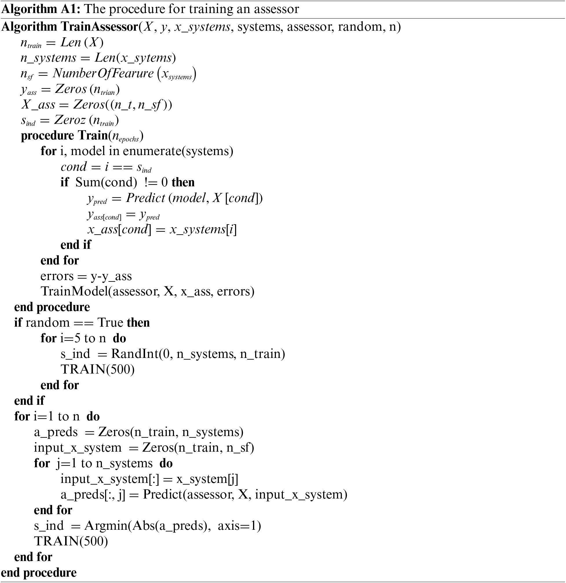
First, 30 randomly generated systems were trained on the training set, and then how the assessor model assessed these systems was investigated by averaging the results over the examples. Each system is a one-hidden layer NN model with the following architecture shown in Appendix A. Due to the random selection of losses during training systems, we remove some systems with NaN (Not a Number) loss values or some systems’ average PIP is less than a threshold value on the training set3. After omitting these systems, we have left several systems, so the assessor accuracies on a system whose average PIP is the highest4 are shown in Fig. 1 over 59 test sets, and the first set is used to train the assessor model. The detailed setups and steps of the training assessor model are described in Appendices B and C.

Figure 1: Average assessor accuracies on 59 test sets by four metrics

In Fig. 1, all accuracies are close to 1 except the balanced one. According to these accuracies, the developed assessor model usually predicts well; it reaches near one on a few test sets without dispatching the considered system. Nevertheless, this assessor performance for a system with the lowest average PIP significantly differs from that in Appendix D, as both systems have various behaviors.

Typically, all rates in the latter scenario are markedly higher than in the former. This occurrence is similar to the class imbalance problem in classification settings because the assessor model suffers from few error responses produced by exceptionally reliable systems. This issue also occurs in the proposed feedback mechanism for the best and selected systems while not for the worst system demonstrated in Fig. 2; the corrections have contrasting effects. As the chosen system for each input instance is determined by the assessor’s identification of the lowest error, this phenomenon does not exert a significant negative impact but manifests in highly accurate models.

Figure 2: Regression output correction by the assessor

After correcting the model outputs, the worst system outperforms two out of nine systems, and the rest of the errors are close to the best and selected models. Nevertheless, the correction technique can have little influence on the two systems. In contrast to these outcomes, we see better results for classification problems in the following subsection. Both results are produced on various feedback truncation rules than Eq. (4), as detailed in Appendix B

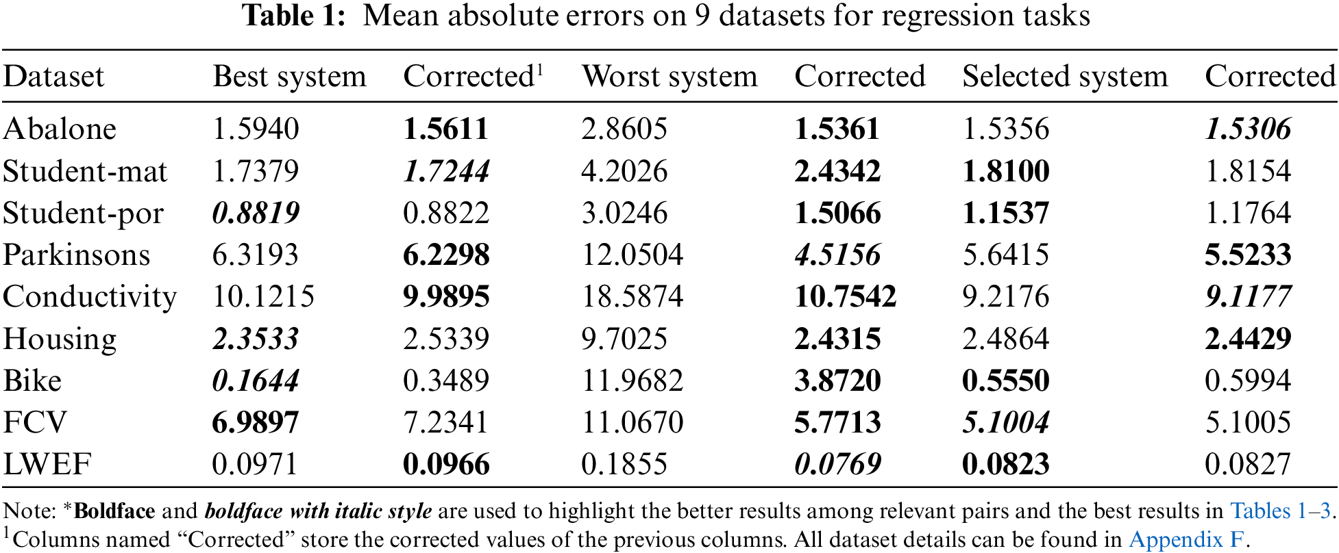
Furthermore, Table 1 presents additional findings regarding regression tasks across various datasets. Similarly, the preceding results in the regression corrections shown do not demonstrate improvement for “the best” and “the selected” systems. However, they positively affect the worst systems, with the outcomes being the best in two datasets and comparable in others.

4.3 Classification Task Results

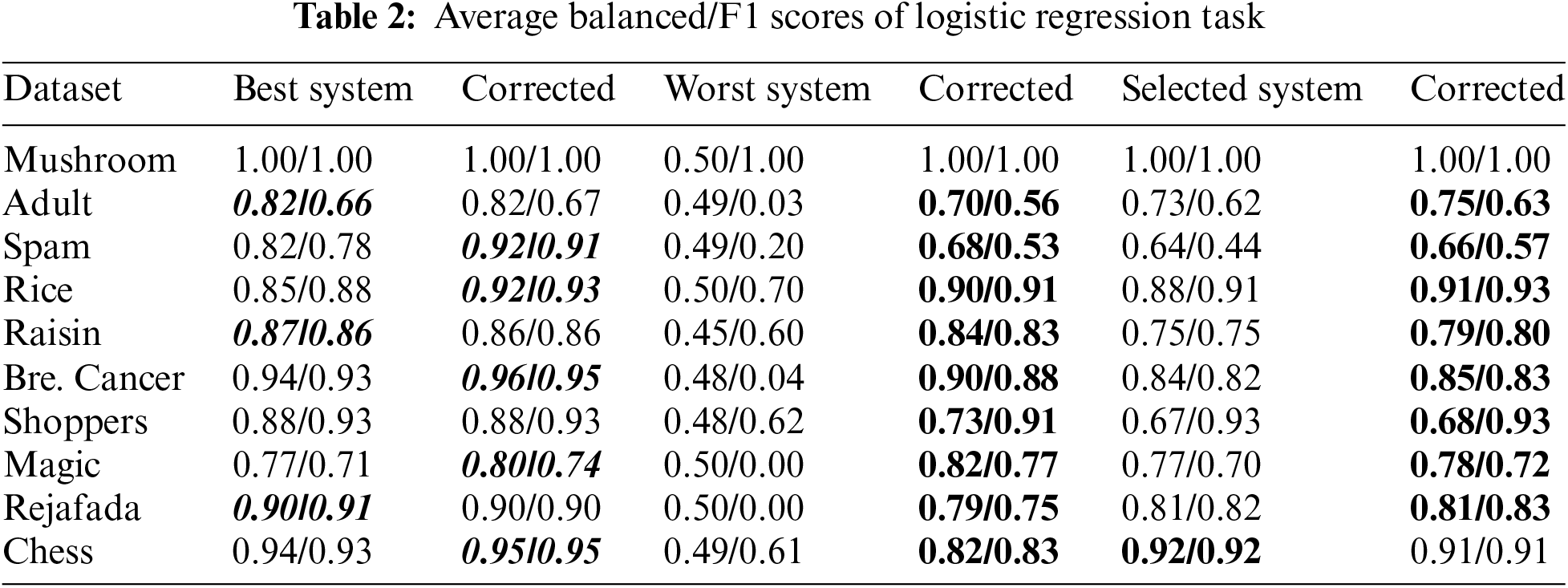
Likewise in the regression task, in this case, we also generate all NN models with only one hidden layer randomly and train an assessor model on their error responses across datasets. However, the assessor model is not as large as in the regression. We utilized 10 datasets to showcase the results of the proposed methodology in balanced and F1 scores presented in Table 2 for binary classifications. In most cases in Table 2, the feedback produced by the assessor model has affected on the values of both metrics considerably well (i.e., negative effects occurred on only three datasets for the best system and one dataset for the selected system).

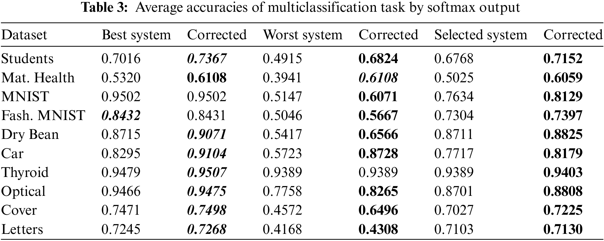
To demonstrate the results for softmax output, we apply the proposed approach for multiclassification problems, and likewise the earlier experiments, we also employ NN models in the same manner. As described in the preceding section, we encode class labels into their one-hot form. For example, the true labels are encoded as y=[0,0,…,1,…,0], the respective predicted ones as y^=[0.02,0.05,…,0.95,…,0], and the errors are computed as yerror=y−y^=[−0.02,−0.05,…,0.05,…,0]. Since the error term in this task is not a scale similar to preceding both experiments, we sum absolute values of yerror to prefer and decide whether an ML model can succeed on a particular example. In turn, our assessor model also produces multiple outputs for each class. Table 3 presents the outcomes of the proposed method on this task. Analogous to outcomes in Table 2, error correction increased the average accuracies of most systems on almost all datasets, except in two cases: MNIST and Fashion MNIST for the best model.

5  Discussion

Assessors were initially introduced to elucidate the behaviors of AI models, mitigating their unpredictable decisions on each new incoming instance. Before deploying them, we can utilize assessors to evaluate whether a system functions correctly, determining the probability of success or failure. Retaining all the attributes of assessors, the proposed method transforms the probability into an error term, which serves as the training input for the assessor meta-model. This model provides feedback for each case to rectify the outputs. The first challenge here is to construct a vector that explains the emergent characteristics of predictors. This work builds it from NN model architectures and other hyperparameters relevant to the training process. A broad range of provided computational research results shows that the current approach has considerable positive outcomes for inaccurate systems along with notable increases for more accurate models. The rationale behind this might be that each dataset should be treated individually, which is also associated with calibration concerns. This study employs nearly identical architectures across all datasets.

This constraint primarily pertains to regression problems. While reducing errors in less accurate systems also elevates errors in other systems. Nonetheless, as depicted in Fig. 1 for 59 test sets, there is a slight improvement, as evidenced in Table 1. Specifically, this constraint is observed in only 8 out of 18 cases, yet most values are very similar. Moreover, in the final two task categories, the results presented in Tables 2 and 3 exhibit notable improvement compared to the regression task.

Analyzing the limitations of the proposed approach is worthwhile, given that the method has not yet been theoretically guaranteed. Initially, we partitioned datasets into three segments: training (for ML model training), validation (to create an assessor dataset), and testing (for assessor evaluation), using seeds that may vary. In specific configurations, we encountered outcomes that were not advantageous. Nevertheless, conducting research across multiple datasets necessitates meticulous implementation of both models and assessors tailored to each domain5 . Another limitation is that the bigger architecture of assessors is utilized compared to the systems to calibrate two inputs6. We hope that if tasks demand more complex ML models, then the lack disappears since the application in [24] is a tiny Random Forest model that helps to train Large Language Models. Finally, the study exclusively utilized NN and SVM-based models, indicating that adapting it to other models would require additional research, which could be identified as future work.

5.1 Ablation Study

Other models. We conducted analogous experiments employing SVM models for regression and classification tasks on the datasets. However, the behaviors of SVM models differ from those of NN models, resulting in diverse outcomes, as illustrated in Appendix E. Individual datasets and models require distinct approaches when selecting mechanism components.

Truncations. Truncation systems7 is one way to balance a dataset on which we train an assessor model whereas, Truncating high errors8 by particular systems mitigates sudden instabilities of the assessor model since these values are targets for assessor datasets. Ultimately, with both ML models and a meta-model, an assessor trained on the responses of these models, we need to address two uncertainties: those of the ML models and the assessor. As a solution, we specifically introduced a truncation function in Eq. (3), such as Eq. (4), detailed in Appendix G. Without feedback truncations, the proposed method could prove ineffective, yielding unfavorable outcomes, as demonstrated in Table A6.

Broader impacts. Modifying the assessor models’ original concept makes it possible to harness their capabilities. It opens up new research avenues, complementing existing ones outlined in [7], including failure explanation, maintenance, and revision. For instance, this could represent a novel step toward ensemble learning and AutoML, aiming to preempt ML model failures and address their inaccuracies in detail. Specifically, employing each weak learner with an assessor model is a potential avenue for future research, particularly in bootstrap aggregating.

6  Conclusion

We proposed an approach to enhance the advent of assessor models by introducing the error term instead of probabilities on a particular instance. This enables us to solve two relevant problems jointly to explain the behaviors of AI models as examples of ML models. The empirical findings underscore the benefits of the proposed method and the challenges that require resolution in future work.

Acknowledgement: Not applicable.

Funding Statement: This work is supported by BK21 Four Project, AI-Driven Convergence Software Education Research Program 4199990214394 2, and also supported by National Research Foundation of Korea 2020R1A2C101 2196.

Author Contributions: The authors confirm contribution to the paper as follows: study conception and design: Musulmon Lolaev, Anand Paul; data collection: Musulmon Lolaev; analysis and interpretation of results: Anand Paul, Jeonghong Kim; draft manuscript preparation: Musulmon Lolaev, Anand Paul, Jeonghong Kim. All authors reviewed the results and approved the final version of the manuscript.

Availability of Data and Materials: Data openly available in a public repository. The data that support the findings of this study are openly available in the UCI Machine Learning Repository at https://archive.ics.uci.edu/ (accessed on 17 November 2024) and Appendix F.

Ethics Approval: Not applicable.

Conflicts of Interest: The authors declare no conflicts of interest to report regarding the present study.

1Nevertheless, AutoML searches several AI models and evaluates them based on some metrics according to the considered tasks. It usually suggests one of these models while the assessor models evaluate them based on each instance separately. If the task is selecting a system, the assessor selects a system for each instance separately based on success rate. In contrast, AutoML chooses only one system for generalization metrics, such as accuracy or loss on test sets.

2In this case, we suppose that the task of the assessor mode is selecting the best model. In general, we can select any system out of the systems, and we fix its error.

3According to PIP in Eq. (5), it is computed based on the predicted error by the assessor for pair (Si, Xj). If we replace the predicted error with the true error after acquiring an output of system i on object j and average it over examples in the training set, we calculate the average PIP for system i.

4In the rest of the paper, we refer to a system with the highest PIP as “The best system,” and a system with the lowest PIP as “The worst,” and a system selected by the assessor model concentrating the lowest error for each input instance as “The selected system”.

5The complete source code is located in the link.

6In all settings, the calibration has only been adjusted for the feedback mechanism, not for selection models. Therefore, the best models based on average accuracy are more accurate than the selected ones by assessors.

7Dropping less accurate systems is natural since we do not prefer them in practice.

8We only applied truncations for regression tasks with values of 70, 50 for the first and second regression results.

References

1. A. Krizhevsky, I. Sutskever, and E. G. Hinton, “Imagenet classification with deep convolutional neural networks,” Commun. ACM, vol. 60, no. 6, pp. 84–90, 2012. doi: 10.1145/3065386. [Google Scholar] [CrossRef]

2. J. Li, “Recent advances in end-to-end automatic speech recognition,” 2022, arXiv:2111.01690. [Google Scholar]

3. F. Stahlberg, “Neural machine translation: A review and survey,” J. Artif. Intell. Res., vol. 69, pp. 343–418, 2020. doi: 10.1613/jair.1.12007. [Google Scholar] [CrossRef]

4. X. Fang and J. Zhan, “Sentiment analysis using product review data,” J. Big Data, vol. 2, no. 5, 2015. doi: 10.1186/s40537-015-0015-2. [Google Scholar] [CrossRef]

5. D. Dasgupta, D. Venugopal, and K. Gupta, “A review of generative ai from historical perspectives,” 2023. doi: 10.36227/techrxiv.22097942. [Google Scholar] [CrossRef]

6. D. Amodei, O. Christopher, J. Steinhardt, P. Christiano, J. Schulman and D. Manê, “Concrete problems in AI safety,” 2016, arXiv:1606.06565. [Google Scholar]

7. J. Hernandez-Orallo, W. Schellaert, and F. Martinez-Plumed, “Training on the test set: Mapping the system-problem space in ai,” Proc. AAAI Conf. Artif. Intell., vol. 36, no. 111, pp. 12256–12261, 2022. [Google Scholar]

8. J. Mislav, S. Agneza, and B. Mario, “AI safety: State of the field through quantitative lens,” in 43rd Int. Conv. Inf., Commun. Electron. Technol. (MIPRO), 2020, pp. 1254–1259. [Google Scholar]

9. S. Han, C. Lin, C. Shen, Q. Wang, and X. Guan, “Interpreting adversarial examples in deep learning: A review,” ACM Comput. Surv., vol. 55, 2023. doi: 10.1145/3594869. [Google Scholar] [CrossRef]

10. K. Alexey, I. Goodfellow, and S. Bengio, “Adversarial examples in the physical world,” in Pro. ICLR 2017, 2017. [Google Scholar]

11. H. Liang, E. He, Y. Zhao, Z. Jia, and H. Li, “Adversarial attack and defense: A survey,” Electronics, vol. 11, no. 8, 2022, Art. no. 1283. doi: 10.3390/electronics11081283. [Google Scholar] [CrossRef]

12. L. Schwinn, D. Dobre, S. Günnemann, and G. Gidel, “Adversarial attacks and defenses in large language models: Old and new threats,” 2023, arXiv:2310.19737. [Google Scholar]

13. F. Martínez-Plumed, D. Castellano, C. Monserrat-Aranda, and J. Hernández-Orallo, “When AI difficulty is easy: The explanatory power of predicting IRT difficulty,” Proc. AAAI Conf. Artif. Intell., vol. 36, no. 7, pp. 7719–7727, Jun. 2022. doi: 10.1609/aaai.v36i7.20739. [Google Scholar] [CrossRef]

14. O. Wiles et al., “A fine grained analysis on distribution shift,” 2021, arXiv:2110.11328. [Google Scholar]

15. T. Fujimoto, J. Suetterlein, S. Chatterjee, and A. Ganguly, “Assessing the impact of distribution shift on reinforcement learning performance,” 2024, arXiv:2402.03590. [Google Scholar]

16. J. S. Bridle, Probabilistic Interpretation of Feedforward Classification Network Outputs, with Relationships to Statistical Pattern Recognition, F. F. Soulié, J. Hérault, Eds. Berlin, Heidelberg: Springer Berlin Heidelberg, 1990. [Google Scholar]

17. K. Kumar, C. Vishnu, R. Mitra, and C. Mohan, “Black-box adversarial attacks in autonomous vehicle technology,” in 2020 IEEE Appl. Imagery Pattern Recognit. Workshop (AIPR), 2020, pp. 1–7. [Google Scholar]

18. R. Fabra-Boluda, C. Ferri, F. Martínez-Plumed, and J. Ramírez-Quintana, “Robustness testing of machine learning families using instance-level IRT-difficulty,” in EBeM’22: Workshop on AI Evaluation Beyond Metrics. Vienna, Austria: RWTH Aachen University, Jul. 25, 2022, vol. 107. [Google Scholar]

19. M. Smith, T. Martinez, and C. Giraud-Carrier, “An instance level analysis of data complexity,” Mach. Learn., vol. 95, no. 2, pp. 225–256, 2014. doi: 10.1007/s10994-013-5422-z. [Google Scholar] [CrossRef]

20. C. Thornton, F. Hutter, H. H. Hoos, and K. Leyton-Brown, “Auto-WEKA: Combined selection and hyperparameter optimization of classification algorithms,” in Proc. 19th ACM SIGKDD Int. Conf. Knowl. Discov. Data Mining, New York, NY, USA, Association for Computing Machinery, 2013, pp. 847–855. doi: 10.1145/2487575.2487629. [Google Scholar] [CrossRef]

21. F. Hutter, L. Kotthoff, and J. Vanschoren, “Automatic machine learning: Methods, systems, challenges,” in Challenges in Machine Learning. Germany: Springer, 2019. [Google Scholar]

22. Z. Chen and H. Ahn, “Item response theory based ensemble in machine learning,” Int. J. Autom. Comput., vol. 17, no. 5, pp. 621–636, 2020. doi: 10.1007/s11633-020-1239-y. [Google Scholar] [CrossRef]

23. C. Oliveira and R. Prudêncio, “Item response theory to evaluate speech synthesis: Beyond synthetic speech difficulty,” in EBeM’22: Workshop on AI Evaluation Beyond Metrics. Vienna, Austria: CEUR Workshop Proceedings, Jul. 25, 2022, vol. 107. [Google Scholar]

24. L. Zhou, F. Martínez-Plumed, J. Hernández-Orallo, C. Ferri, and W. Schellaert, “Reject before you run: Small assessors anticipate big language models,” in EBeM’22: Workshop on AI Evaluation Beyond Metrics. Vienna, Austria: RWTH Aachen University, Jul. 25, 2022, vol. 107. [Google Scholar]

25. C. Corbière, N. Thome, A. Bar-Hen, M. Cord, and P. Pérez, Addressing Failure Prediction by Learning Model Confidence. Red Hook, NY, USA: Curran Associates Inc., 2019. [Google Scholar]

26. K. Buza, “Feedback prediction for blogs,” in Data Analysis, Machine Learning and Knowledge Discovery. Germany: Springer, Aug. 2021, pp. 145–152, 2014. [Google Scholar]

27. D. Dua and C. Graff, “UCI machine learning repository,” Accessed: Nov. 17, 2024. [Online]. Available: https://archive.ics.uci.edu/ [Google Scholar]

Appendix A. Neural Network Architecture Properties

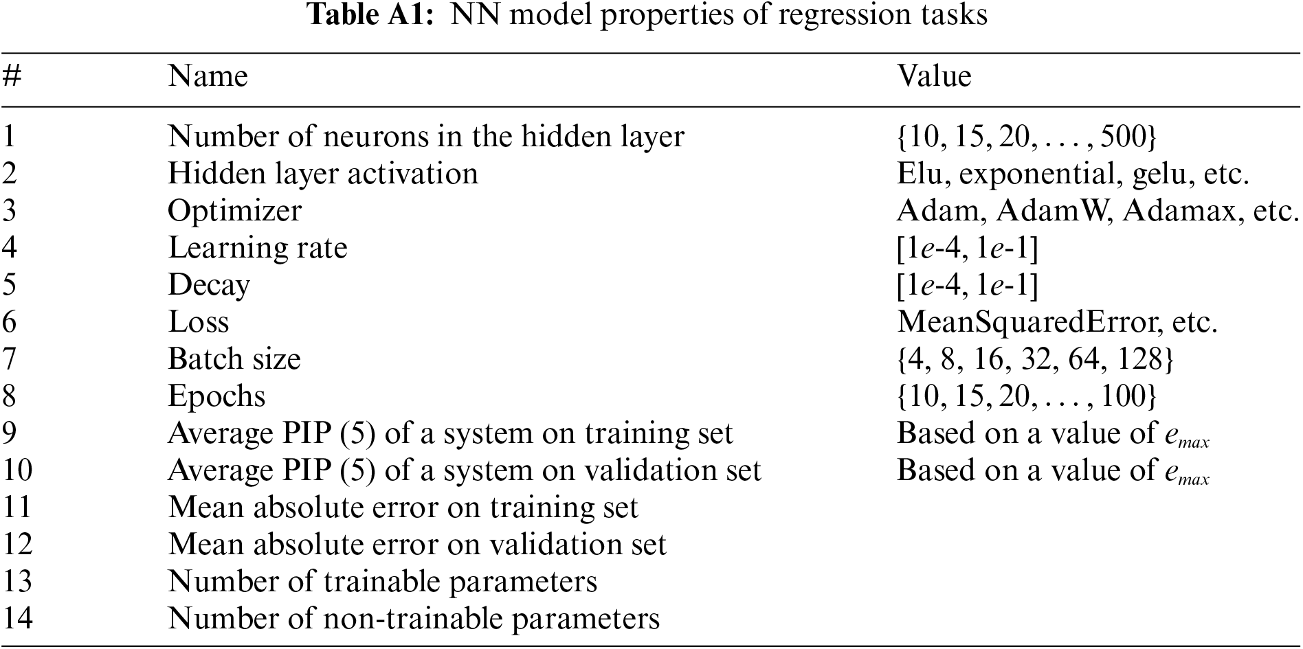
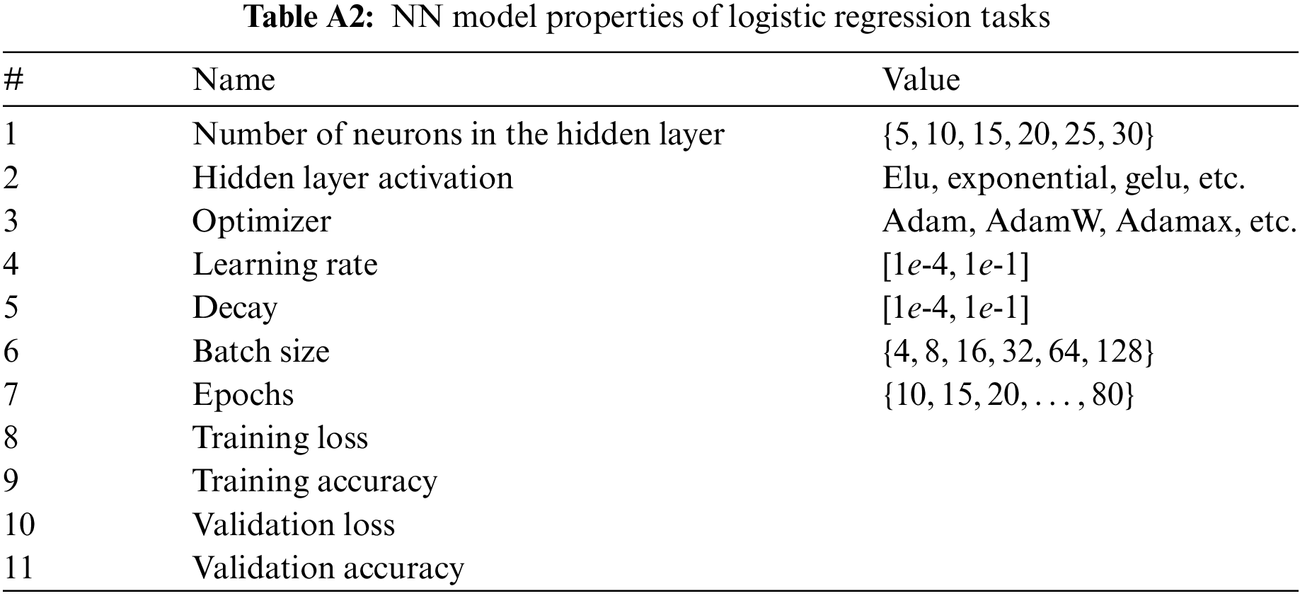
Table A1 presents each NN regression model built with a single hidden layer by randomly selecting its parameters. These parameters that describe the emergent behaviors of systems are so flexible that we can modify them regarding our task. However, they have to save all properties of the assessor model. Table A2 also illustrates the same parameters for logistic regression and softmax outputs. We built each NN regression model with a single hidden layer by randomly selecting its parameters presented in Table A1.

Appendix B. Neural Experimental Setups and Details

While producing research results, we leveraged two different setups for regression and logistic regression with multiclassification tasks due to the difference between datasets. In both setups, we first generated NN models (numbers of models may vary in different tasks on datasets) according to their system features presented in Tables A1 and A2. Next, we train them on the training sets and check their performance on validation sets to complete their behavior values, such as validation scores. Once we have trained systems, we truncate them regarding their performance. Finally, we produce the error responses from randomly selected systems on the training sets to warm up the assessor model, and we then train the assessor model on error returns from the validation sets.

During the training, we used the early stopping strategy with different values for systems and assessors. Therefore, the initial randomly selected epochs also changed according to this, and we updated the relative values of systems. The dataset used in the regression task has few values significantly greater than most examples. This circumstance generated a few huge errors (target truncation) that caused the assessor model to be trained inconsistently over batches of examples. To mitigate this challenge, we truncated the errors with a threshold 70. However, this problem can only occur in part of the two tasks. Moreover, feedback truncation is applied as the following equation for the first experiment, Blog feedback dataset:

for the best and selected systems, ftrun(e^ji)={e^jiif|e^ji|≤7.50otherwise;

for the worst system, ftrun(e^ji)={e^jiif|e^ji|≥50otherwise.

The equations for the second regression experiment on 9 datasets are shown in Table A1 (in Section 4.2):

for the best and selected systems, ftrun(e^ji)={e^jiif|e^ji|≤0.25emax0otherwise;

for the worst system, ftrun(e^ji)=e^ji.

Experimental parameter settings. In the first research, we set up the following: the number of randomly generated systems to truncate less accurate systems was used, and the random seed. Since the maximum value of the dataset target is, that is an appropriate value. The parameters of logistic regression and multiclassification tasks varied significantly in different datasets. Due to the randomness, the presented results will vary even in the same settings. Tables A3–A5 illustrate the number of neurons and parameters during the experiments in Tables 1–3 (in Section 4). Additionally, in all problems, we use the same random parameters: learning_rates = linspace (1e-5, 1e-1, 50), weigth_decays = linspace (1e-5, 1e-1, 50), epochs = range (10, 80, 5), batch_size z = [4, 8, 16, 32, 64, 128], 30 random models, random seed = 42 for all datasets. Note that the seed value, 42, is only used in datasets into three subsets: training, validation (also for collecting responses for assessor datasets), and testing for testing assessors’ performances.

Appendix C. The Procedure for Training an Assessor

Algorithm A1 trains an assessor model by collecting error responses from a given ML population and dataset. Initially, we do not know which model produces lesser error than others, so we train an assessor on errors produced by randomly selected models. In this, we assume that we have some functions. The complete code of the implementation can be found in the https://anonymous.4open.science/r/ass-feedback-616Clink, accessed on 18 October 2024.

Appendix D. Average Accuracies of the Worst System

All scores in some sets are close to 70%. Therefore, the assessor works quite well for this system, as shown in Fig. A1.

Figure A1: Average assessor accuracies of 59 test sets by 4 metrics for the worst system

Appendix E. Results of Other Models

For the ablation study, we also included SVM-based models to illustrate the advantages and disadvantages of the proposed work. To implement using SVM, we leveraged scikit-learn library. As emergent behaviors of models, the hyperparameters: kernel types (‘linear’, ‘rbf’, ‘poly’, ‘sigmoid’), C (regularization term, range (1, 50, 1)), degree of the polynomial kernel range (1, 10, 1), coefficient linspace (0, 0.2, 10), tolerance linspace (1e-3, 1e-2, 10), training accuracy and validation accuracy are used to describe SVM-classification models. For regression tasks, we only included mean absolute errors on training and validation tests. The rest of the settings are the same as the NN models described in the central part of the work. For instance, we trained the assessor models using Algorithm A1. Table A6 illustrates the outcomes in various settings. The last column of the table, ‘truncation values,’ is feedback truncation. Note that the seed value, 42, is only used to divide datasets into three subsets: training, validation (also for collecting responses for assessor datasets), and testing for reporting assessors’ performances.

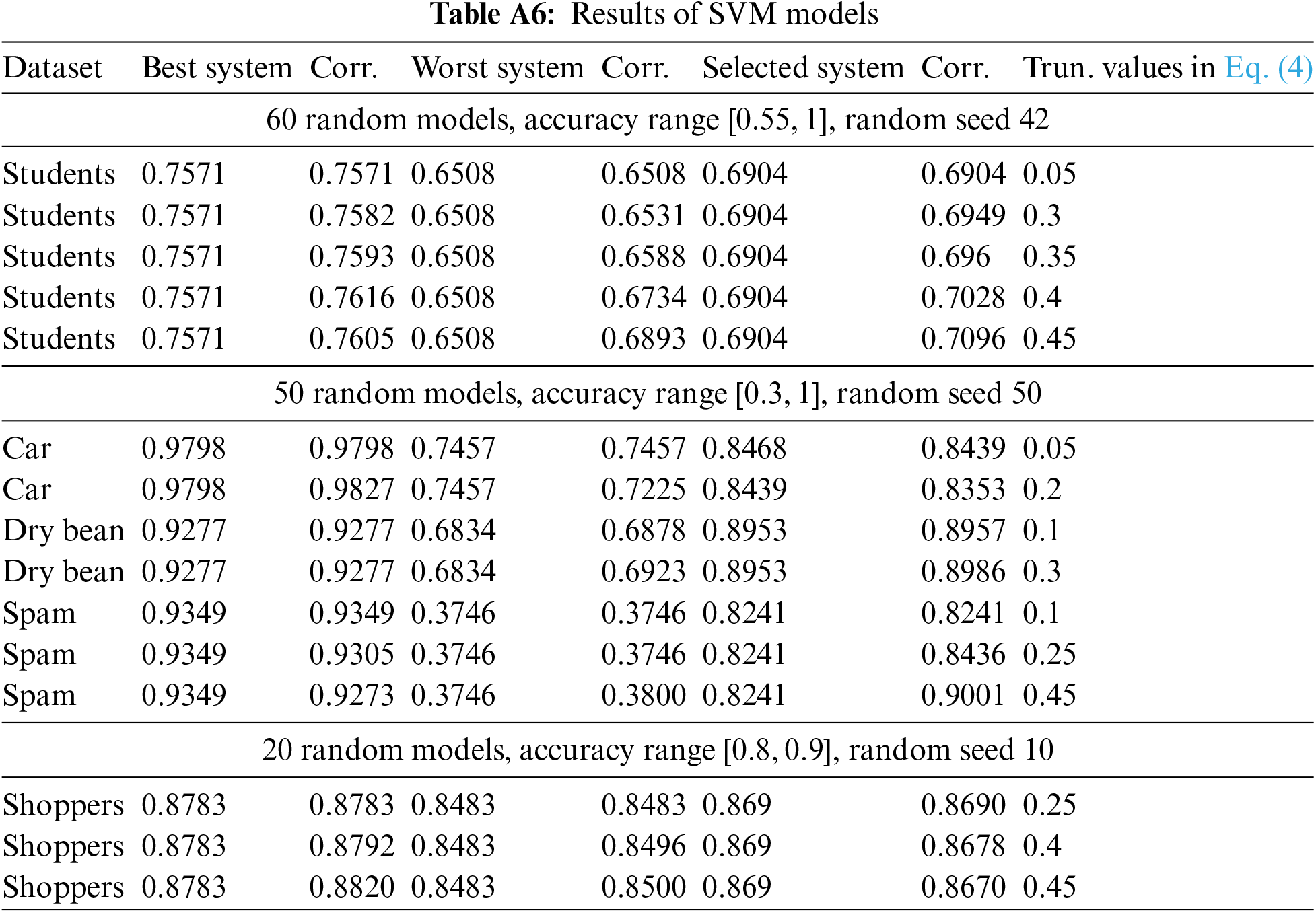
Truncation effects. The table stores a range of examples with various settings to illustrate how truncations are helpful. In the first setting, all error mitigations are positive from 5% to up to 45%, whereas they are only slightly better for the best model in the second setting and not valid for other models.

Appendix F. Datasets

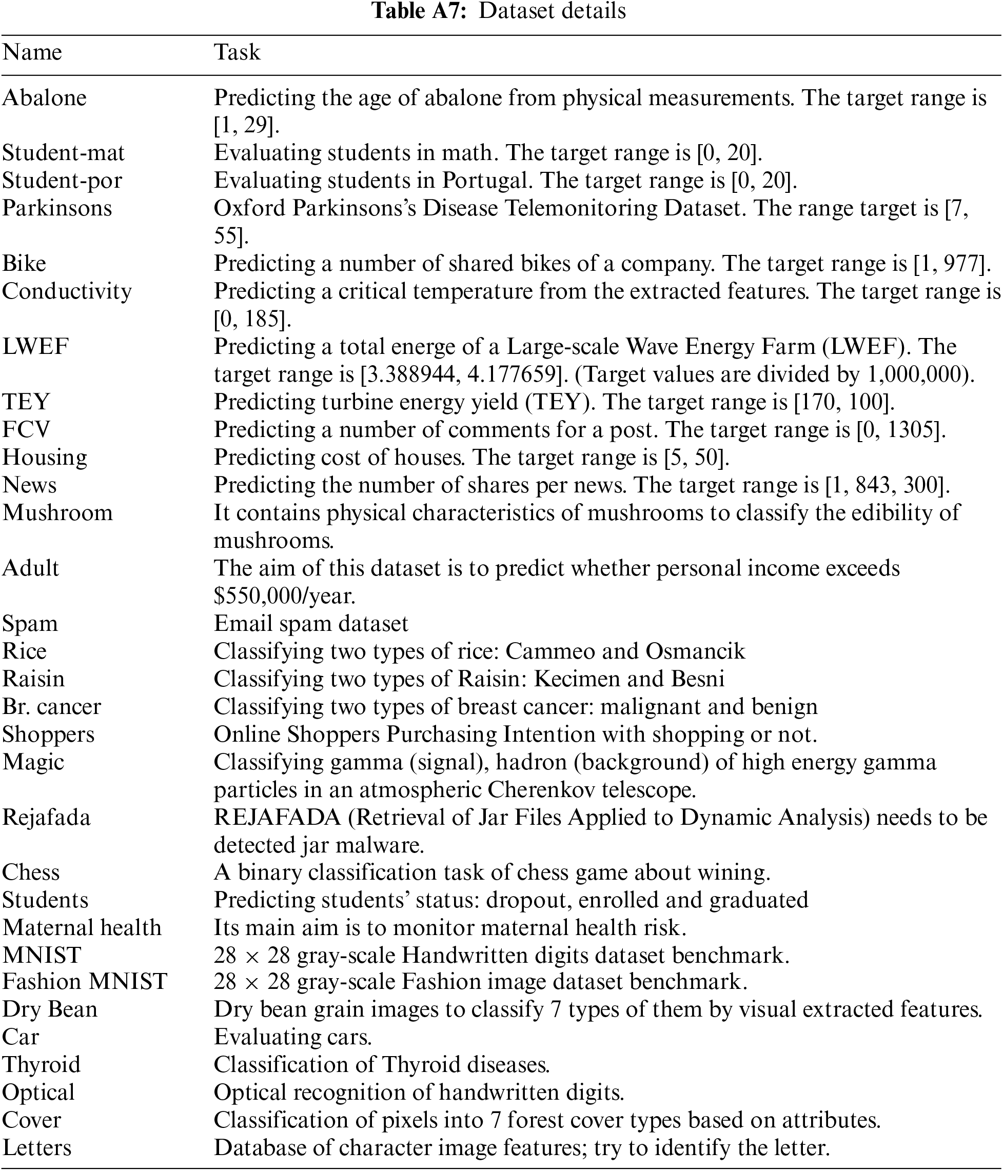
All used datasets are well-known and publicly available to leverage in research works. Most of them are downloaded from [27] (UCI), and the number of instances in each dataset is more than 500, up to 581,000 for better evaluation. Table A7 describes all datasets and their external links used in the work.

Appendix G. Truncations

Feedback truncations have been carried out differently for regression and classification tasks. For regression, we use a threshold of 0.25*max_error for only the most accurate and selected systems, not for the worst systems. That is, we do not add predicted errors by assessors to the outputs of worst models. Whereas, for classification tasks, we employ a different approach to adjust the idea for all datasets simultaneously; instead of one threshold, we use thresholds [0.1,0.2,0.3,0.4,0.5] because the output for this task ranges from 0 to 1. While choosing results, we took only the best ones from the five results because we have 20 datasets, and each requires a distinct threshold, which is rare even when altering any hyperparameters. For this reason, the classification results look better than the regressions’. If we remove this truncation, the corrects often are unfavorable, decreasing accuracies instead of increasing.