Weather Classification for Autonomous Vehicles under Adverse Conditions Using Multi-Level Knowledge Distillation

1  Introduction

Autonomous cars, or self-driving vehicles, are transforming sectors like transportation, agriculture, and security by using sensors, perception systems, and artificial intelligence to navigate independently. These cars offer improved road safety, enhanced traffic flow, reduced fuel consumption, and lower pollution. Accurate weather condition awareness is crucial for secure navigation, route decisions, safety assessments, and performance enhancement [1,2]. Classifying weather conditions from images presents several challenges: ambiguity in defining class boundaries, variability in weather appearances, image quality degradation due to adverse weather, and the difficulty of obtaining a diverse, large-scale dataset for robust model training models [3–5].

Traditional weather classification methods use hand-crafted features like colour, texture, and shape descriptors with machine learning algorithms such as Support Vector Machines (SVM). These methods are time-consuming, labour-intensive, and often inaccurate because hand-crafted features may miss subtle weather nuances, and machine learning algorithms may be imprecise if the dataset does not accurately represent real-world conditions [6]. Recent advances in deep learning, particularly using Convolutional Neural Networks (CNNs) like ResNet, VGG, and EfficientNet, have significantly improved image classification tasks, including weather condition classification. These models learn hierarchical representations of images, capturing both low-level and high-level weather features [7–9]. Transfer learning further enhances these models by leveraging pre-trained models on large, non-weather datasets, enabling the models to learn useful general features. This approach facilitates faster convergence, reduces computational demands, and is particularly beneficial when resources or time is limited [10].

The advancement of autonomous vehicles is hindered by limited perception of challenging weather. Plested et al. [11] investigated the effects of various weather conditions on ADS sensors and reviewed state-of-the-art algorithms and deep learning techniques, such as weather classification and remote sensing, that improve perception. It categorizes simulators, experimental facilities, weather-inclusive datasets, and sensor fusion solutions. It also explores V2X communication and potential sensor options for ADS, addressing weather-related perception challenges. Adverse weather conditions like fog, haze, snow, mist, and glare challenge autonomous vehicle vision systems. To ensure safe operation, image dehazing is crucial. Mehra et al. [12] introduced ReViewNet, a fast, lightweight dehazing technology for autonomous vehicle cameras. ReViewNet demonstrated superiority over existing methods through extensive quantitative analysis on five datasets and component-wise ablation tests by incorporating spatial feature pooling, quadruple colour cues, multi-look architecture, and multi-weighted loss function.

Addressing Neural Networks (NNs) challenges in real-world image recognition for autonomous driving, Yu et al. [13] proposed the RobuTS dataset for Robust Traffic Sign Recognition, featuring images with environmental variations like rain, fog, darkening, and blurring. They introduced Robust Training without adverse scenario data (REIN) and Self-Teaching (ST) with unlabeled adverse data, reducing data collection and annotation needs. These schemes showed significant performance improvements, with REIN achieving 15%–25% and ST achieving 16%–30% in classification tasks. The paper [13] presented a deep learning-based framework for classifying weather conditions to aid autonomous vehicle decision-making, especially in adverse situations. Using transfer learning, it evaluates three deep CNNs, SqueezeNet, ResNet50, and EfficientNet, on a dataset combining DAWN2020 and MCWRD2018 with six weather classes. ResNet50 achieved the highest metrics with 98.48% accuracy, 98.51% precision, and 98.41% sensitivity. Despite attaining a marginally lower accuracy than [14], it is noteworthy that our work has extended the classification to encompass seven classes, compared to the six classes used in their study.

Vehicle detection challenges in traffic management, focusing on both day and night conditions using fast R-CNN, is proposed in [15], which demonstrates improved performance in various scenarios, including low illumination and long shadows, achieving an average accuracy of 94.20% and precision of 90%. A modified Cascade RCNN is introduced [16] for vehicle detection, enhancing the feature pyramid and integrating context information to improve detection accuracy. The method shows a 2.82% and 2.89% improvement for small and medium objects, respectively, and a 90.57% accuracy for large objects, effectively addressing detection challenges for small and occluded vehicles. The study [17] introduced MeteCNN, a new deep-learning model for classifying weather phenomena in images. The WEAPD dataset, created for this research, boasts more categories than prior efforts. MeteCNN achieves impressive accuracy (around 92%) on WEAPD, displaying its potential for future weather prediction and image classification tasks.

Muşat et al. [18] highlighted the impact of adverse weather on sensors like Lidar, GPS, cameras, and radar, noting significant performance reductions, such as a 45% decrease in mm-wave radar range during heavy rain. Addressing these issues can enhance autonomous vehicle performance in such conditions. In [19], polarimetric imaging improved road scene analysis under adverse weather, providing a 15%–44% performance boost in foggy conditions by combining polarimetric images with a tailored learning model. A visibility enhancement scheme was proposed [20], and a robust vehicle detection and tracking method using a multiscale deep convolutional neural network. Tested on DAWN, KITTI, and MS-COCO datasets, the method outperformed others, significantly improving detection in fog, rain, snow, and sand by 10.36%, 13.94%, 21.46%, and 15.17%, respectively.

Oluwafemi et al. [21] utilized a stacked ensemble algorithm, Selection Based on Accuracy Intuition and Diversity (SAID), employing histogram features to classify various weather scenes. This method achieved an accuracy of 86% across four classes. Ibrahim et al. [22] proposed a WeatherNet framework where different classes are trained separately using ResNet50 due to the distinct characteristics of the images. This approach resulted in a notable accuracy of 97.69% with four classes. In contrast, Wang et al. [23] explored nine classes using CNN variants such as ResNet50, ResNet101, and DenseNet121 but only attained an accuracy of 81.25%, which is suboptimal by contemporary standards. Xia et al. [24] and Al-Haija et al. [25] implemented variations of ResNet, specifically ResNet15 and ResNet18, achieving accuracies of 96.03% and 98.20% respectively for four classes. The study in [17] employed DeepMeteCNN with eleven classes and achieved an impressive accuracy of 92%. However, despite the public availability of the dataset from Xiao et al. [17], it was designed explicitly for weather classification and does not meet our specific objective of classifying weather conditions for autonomous vehicles. Consequently, we chose not to use this dataset, opting to gather and analyze data explicitly tailored to the context of autonomous vehicles.

MLKD [26] is a deep learning technique for transferring knowledge from complex teacher models to smaller student models, known as distillation. Using a student model reduces model size, memory use, and computational needs while maintaining accuracy. MLKD includes response-based, relation-based, and feature-based distillation, which can be performed offline or online. Response-based MLKD (R-MLKD) learns from the teacher models’ SoftMax output, relation-based MLKD captures class relationships, and feature-based MLKD uses feature representations. Offline distillation uses pre-trained, fixed teacher models, whereas online distillation trains teachers and students simultaneously, offering greater computational efficiency [27] ResNet50V2 [28] and EfficientNetV2B3 [29] are notable pre-trained CNNs used as teacher models. ResNet50V2 uses skip connections to improve gradient flow, while EfficientNetV2B3 balances model size and performance with compound scaling and multi-level feature representations.

Authors in [30] proposed a novel teacher-student model to enhance medical image denoising. Their model incorporates a NoiseContextNet Block and an Attention-based Depth-wise Convolution Network (ADWC) to improve image quality. The staggered distillation technique is crucial, optimizing knowledge transfer while maintaining computational efficiency. Evaluated on diverse datasets, including Chest X-rays, Heart MRI, AAPM, and abdominal CT, the model demonstrated superior performance. Notably, it achieved impressive Structural Similarity Index Measure scores of 95.49% and 96.57% on Heart MRI and abdominal CT, respectively.

Furthermore, the model consistently outperformed other Peak Signal-to-Noise Ratio (PSNR) methods, confirming its effectiveness. A knowledge distillation (KD) framework for efficient facial emotion recognition is proposed in [31]. By distilling knowledge from a computationally intensive Emonet teacher model into lightweight student models (EfficientFormer and MobileNetV2), the proposed method achieves a substantial computational reduction from 4G to 0.3G multiply-accumulate (MAC) operations while maintaining competitive performance. The key innovation lies in a teacher-bounded loss function that effectively combines classification and regression tasks, enhancing both accuracy and efficiency. Evaluated on the AffectNet dataset, the model demonstrates impressive results, achieving accuracies of 73.62% and 73.36% for facial expression classification and RMSE values around 0.3 for valence, arousal, and MAC estimation.

The paper [32] proposed an advanced system that leverages IoT and deep learning to enhance precision agriculture in India. Integrating intelligent farming techniques, the system automates weather forecasting and field monitoring through wireless sensor data to a web server. It uses Gated Recurrent Units (GRU) to forecast weather conditions with 94% accuracy and ResNet50 for disease detection in crop images, achieving 98% accuracy. This approach improves crop productivity and timely alerts farmers about adverse weather and pest issues, optimizing agricultural output and efficiency. The authors [33] proposed the DoSe framework, which addresses the challenge of catastrophic forgetting in Deep Neural Networks (DNNs) for domain generalization and unsupervised domain adaptation. The framework uses Domain-aware Self-Distillation with batch normalization prototypes to maintain model performance across varying target domains. By enforcing consistency in batch normalization statistics and employing a novel exemplar-based replay buffer, DoSe improves knowledge retention. Experiments on the ACDC dataset show that DoSe achieves a 26% improvement in Domain Generalization, a 14% boost in Unsupervised Domain Adaptation, and a 70% increase in Daytime settings compared to existing methods.

MKT-Net, a multi-level knowledge transmission network designed to enhance object detection in challenging rainy nighttime (RNT) conditions, is proposed in [34]. MKT-Net integrates object detection with rain removal and low-illumination enhancement through three interconnected subnetworks. It utilizes feature transmission modules to improve detection accuracy by aggregating multiscale features. Evaluation of various datasets shows that MKT-Net outperforms existing methods by up to 25.43% in mean average precision on an RNT dataset and 15.26% on the rain in the driving dataset while maintaining high detection speed.

This paper introduces R-MLKD, a framework for improving weather classification in autonomous vehicles through offline distillation with multiple teacher models, including ResNet50V2 and EfficientNetV2B3. These models are selected for their state-of-the-art performance in image recognition, with ResNet50V2 excelling in hierarchical feature extraction and EfficientNetV2B3 optimizing depth, width, and resolution scaling for high-resolution data. The dual-model approach facilitates robust knowledge distillation, ensuring comprehensive feature representation. A vanilla CNN is the student model, benefiting from the distilled knowledge to enhance weather classification accuracy.

The proposed Multi-level Knowledge Distillation (MLKD) framework demonstrates the integration of AI and Big data analysis in solving real-world problems in autonomous vehicles. By leveraging pre-trained models and transfer learning, the study enhances weather classification—a critical task for autonomous vehicle safety and efficiency—highlighting the synergy between AI, data modelling, and analysis. There are too many equations. It is highly recommended that only the most relevant equations be included and that well-known equations be avoided.

This approach is a novel application of R-MLKD in this context. The contributions are:

1.    It proposes R-MLKD, a framework that uses two advanced teacher models, ResNet50V2 and EfficientNetV2B3, to train a CNN student model, enhancing weather classification accuracy for autonomous vehicles.

2.    Evaluate the performance of both individual models and the R-MLKD approach, demonstrating reduced computational complexity, making the method suitable for real-time applications by leveraging pre-trained models and transfer learning.

3.    Employing seven weather condition classes based on real-world images from datasets like Berkeley Deep Drive 100K (BDD100K) [35], Diverse Aerial Weather Dataset (DAWN) [36] and Connected Intelligent Transportation Systems (CITS) traffic alerts [37].

The work is structured as follows: Section 2 reviews recent studies related to our research. Section 3 discusses the materials, models, and methods, including datasets and data augmentation techniques. Section 4 presents the objectives, performance evaluation metrics, and a detailed analysis of R-MLKD results. Section 5 concludes and suggests future enhancements.

2  Architecture and Work Methodology

This section presents the architectures of both the teachers and the students, which collectively form the foundation of the R-MLKD framework.

2.1 ResNet50V2–Teacher 1

ResNet50V2 (Residual Network-50V2) is a CNN architecture commonly used in image classification. It is an improved version of the original ResNet50, designed to enhance performance and address limitations. ResNet50V2, as shown in Fig. 1, comprises convolutional layers, residual blocks, and a global average pooling layer, working with an input image size of 224 × 224. It follows residual learning principles to mitigate the degradation problem in deeper networks, where accuracy decreases due to the vanishing gradient issue.

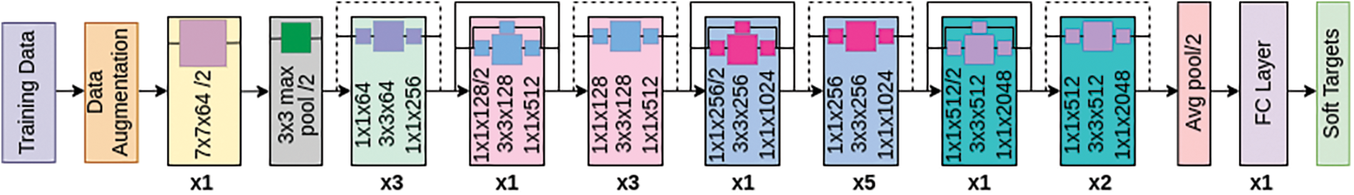
Figure 1: Functional blocks of ResNet50V2

ResNet50V2 is an improvement over ResNet50 [8] in constructing residual blocks. In ResNet50, the residual blocks use the “bottleneck” design, which includes three convolutional layers. On the other hand, as shown in Fig. 2, ResNet50V2 introduces an improved bottleneck design by adding a Batch Normalization (BN) [38] layer before each convolutional layer. This modification enhances the training process and enables better information flow within the network.

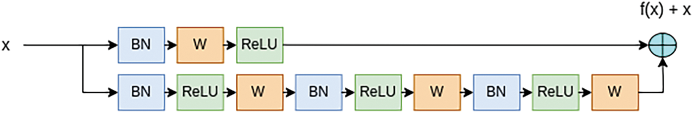
Figure 2: Bottleneck design of ResNet50V2

a) Architecture of ResNet50V2

Shortcut Connections: Also known as identity mappings or skip connections, these allow the network to learn residual functions directly. They preserve original information, mitigating degradation and facilitating deep network training.

Bottleneck Design: This design reduces the input feature maps’ dimensions using convolutions before convolutions. This reduces computational complexity while maintaining representation capacity.

BN: Positioned before each convolutional layer in the residual blocks, BN layers normalize input, reducing overfitting, improving training stability and speed, and enhancing generalization by reducing internal covariate shift. BN is defined by Eq. (1).

(1)

is the input, is the mean, is the variance calculated over the mini-batch, is a small constant for numerical stability, is the scale parameter, and is the shift parameter that is learned during training.

In a residual block in ResNet50V2, which consists of two convolutional layers, batch normalization (BN), and Rectified Linear Unit (ReLU) activation functions, the output is obtained by adding the input directly to the output of the second convolutional layer. Here, the input is passed through the convolutional layers, BN, and ReLU activation, and this transformed output is added to the original input. This process, referred to as a skip connection, allows the network to learn residual functions, making it easier to train deeper networks.

b) Activation function of ResNet50V2

ResNet50V2 primarily utilizes the ReLU activation function, which introduces non-linearity to the network. In this context, the ReLU function returns the input if it is positive and zero otherwise.

AveragePooling2D: Used for down-sampling feature maps by dividing the input into non-overlapping rectangular regions and averaging the values within each region. This reduces spatial dimensions and computational complexity. A stride of 2 cuts spatial dimensions in half.

Flatten and Dense Layers: These are common in both teacher and student models. The flattening layer converts multi-dimensional feature maps into a single vector. The Dense layer, fully connected, links each neuron to every neuron in the previous layer, applying a linear operation followed by a non-linear activation function. The SoftMax function ensures output probabilities sum to one.

2.2 EfficientNetV2B3-Teacher 2

EfficientNetV2B3 is an advanced CNN architecture for efficient image classification and computer vision tasks, with an input size of 300 × 300. Fig. 3 shows the blocks of the EfficientNetV2B3 model derived from [39].

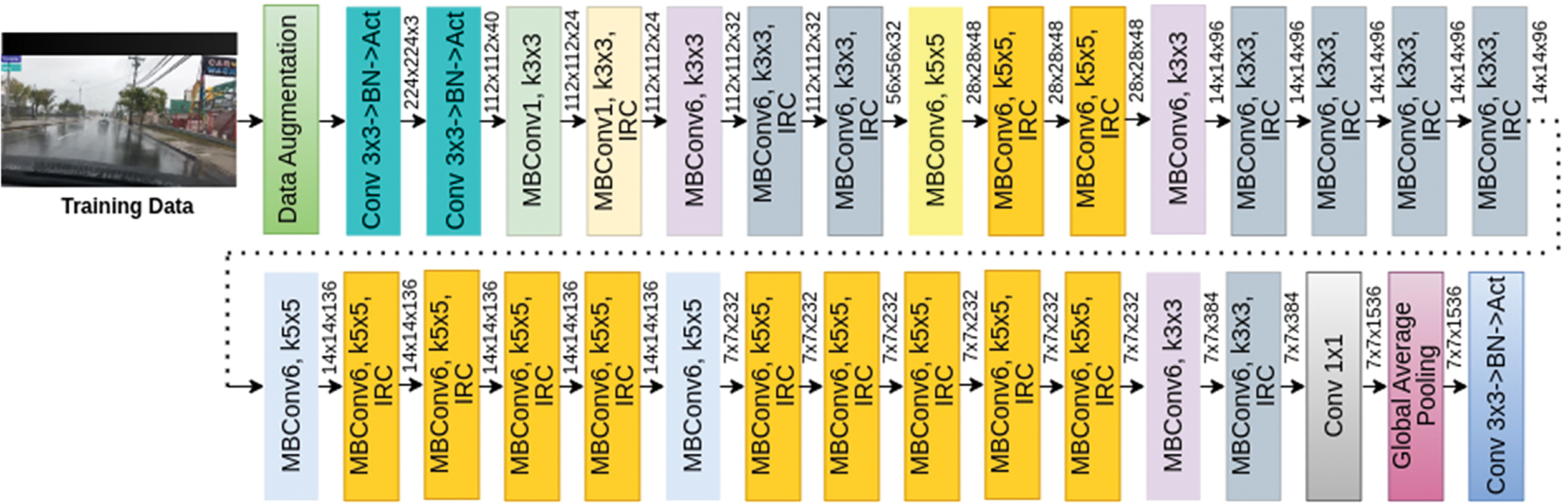
Figure 3: Essential blocks of EfficientV2B3

EfficienetV2B3 is an enhanced version of EfficientB3, featuring compound scaling that simultaneously adjusts network width, depth, and resolution. It includes Squeeze-and-Excitation (SE) modules to improve feature representation. Inverted residual connections link low-resolution feature maps from earlier layers to higher-resolution ones in later layers, enhancing performance with similar parameter counts.

a) Components of EfficientNetV2B3

Stem Convolutional Layers: These initial layers from EfficientNetV2B3 extract low-level features like edges and textures, building a hierarchical image representation.

Stack of Blocks: EfficientNetV2B3 comprises multiple stacked blocks, each including depthwise separable convolutions, SE modules, and inverted residual connections.

Depthwise Separable Convolutions: This method applies filters separately to each input channel (depthwise convolution) and then uses 1 × 1 convolutions (pointwise convolution) to control output depth, significantly reducing parameters compared to standard convolutions. Eq. (2) illustrates depthwise separable convolution, with ∇ representing element-wise multiplication.

(2)

b) Squeeze-and-Excitation (SE) Modules

The SE (Squeeze-and-Excitation) module dynamically adjusts the contribution of each channel based on its importance. It consists of two main operations: squeezing and exciting. The squeezing operation computes channel-wise statistics by globally averaging the input feature maps, which results in a vector representing the importance of each channel. The excitation operation then applies two fully connected layers with a ReLU activation function, followed by a sigmoid activation. This allows the SE module to learn channel-wise excitation weights, which are applied to re-weight the input feature maps, emphasizing informative channels and reducing the influence of less relevant ones.

c) Activation function of EfficientNetV2B3

EfficientNetV2B3 uses the hard Swish activation function, an improved version of ReLU.

2.3 R-MLKD

R-MLKD is a technique used to transfer knowledge from one or multiple teacher networks to a student network, and Fig. 4 shows the framework with two teachers. The goal is to enhance the student network’s performance by leveraging the teachers’ collective knowledge. In this work, ResNet50V2 and EfficienetV2B3 are used as teachers and a basic CNN architecture as a student model. Both teacher networks are trained on the same dataset, and their predictions serve as the source of knowledge for the student network. The knowledge transfer is achieved using the Kullback-Leibler (KL) [40] divergence error. The KL divergence measures the difference between the probability distributions of the teacher networks and student networks’ probability distributions, is robust to overfitting, and allows assigning different probabilities to different classes.

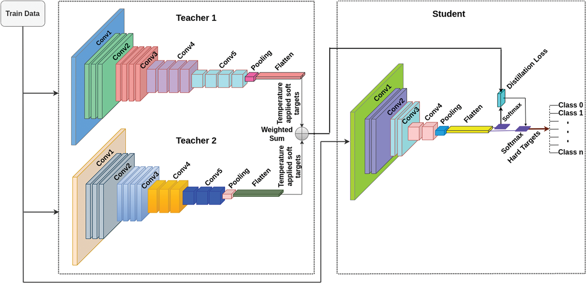
Figure 4: R-MLKD model with two teachers and one student

2.4 Student Model

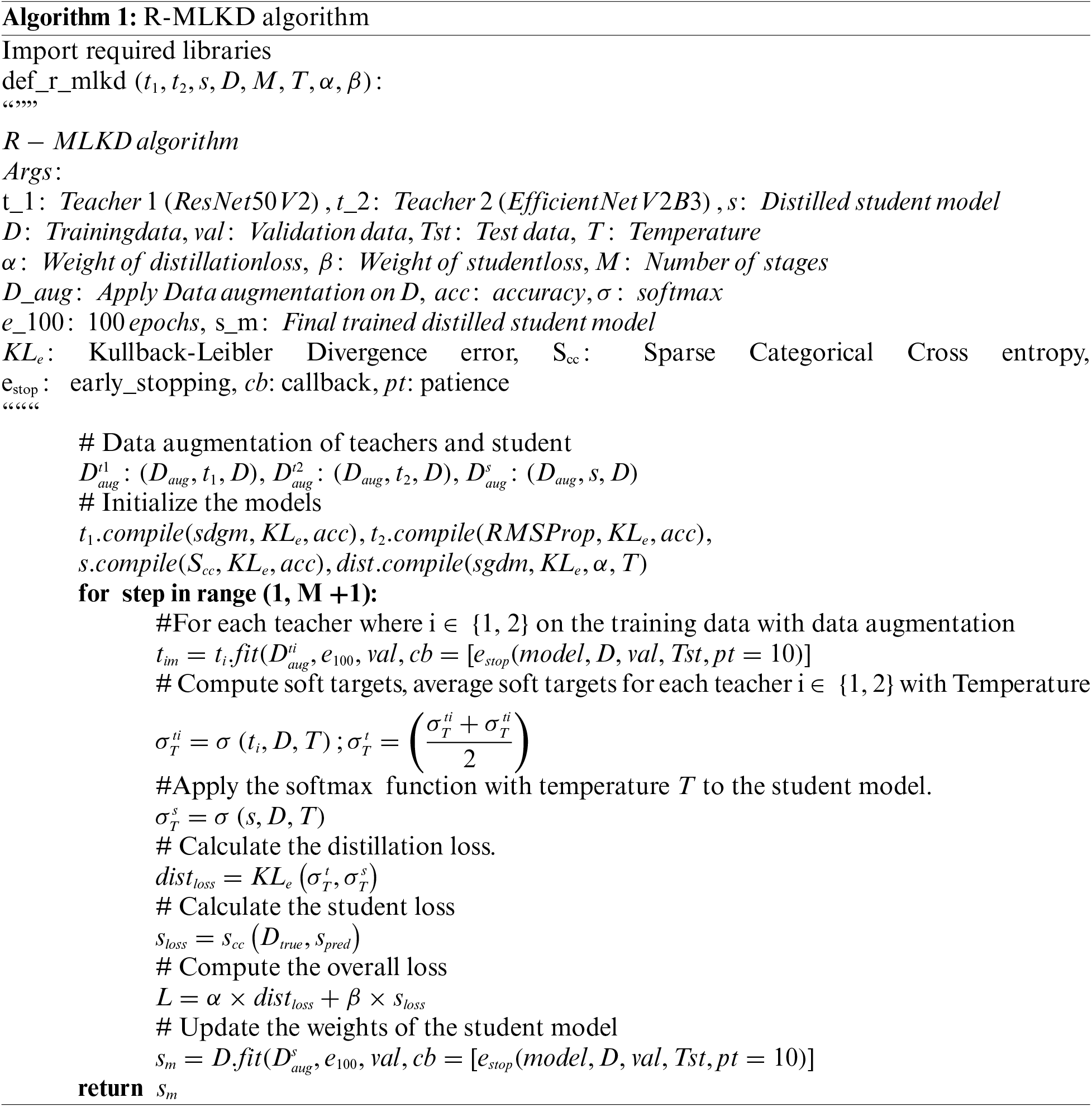
Fig. 5 utilizes visual keras [41] to visually represent the architecture of the student model, which is designed as a simple CNN architecture. The functioning of the proposed R-MLKD is detailed in Algorithm 1. The building blocks of the student model are Conv2D Layer, BN Layer, MaxPooling2D Layer, Dropout, Flatten and a Dense layer. Convolution is a fundamental operation in CNNs that extracts spatial patterns or features from the input data. The Conv2D layer in a CNN performs the convolution operation on the input image using a set of kernels (filters) and produces a feature map. Each filter is a small window that slides across the input image, computing the dot product between the filter weights and the corresponding pixel values in the input.

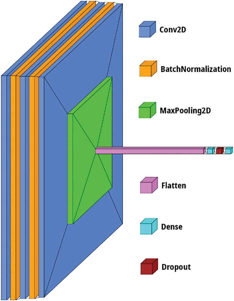
Figure 5: Architecture of student

This dot product operation is performed at each spatial location, resulting in the feature map. The Conv2D layer learns the filter weights during training, optimizing them to detect various local patterns or features in the input image. By stacking multiple Conv2D layers with different filters, the network can capture increasingly complex and abstract features. The operation of the BN layer is like that of ResNet50V2 and MaxPooling2D. The student model is trained to minimize the KL divergence error with respect to the predictions of both teacher networks. By doing so, the student network learns to mimic the combined knowledge of the teachers, allowing it to benefit from their expertise, which helps the student to improve its performance and generalization capabilities.

2.5 Datasets Utilized

This work uses a combination of the seven classes of datasets: fog, overcast, partly cloudy, rain, sandstorm, snow and sunshine.

a) BDD100K (Berkeley DeepDrive 100K)

BDD100K is a large, diverse driving dataset with high-resolution images and videos from various locations and times, including different weather conditions. It includes labelled bounding boxes for six weather classes: foggy, partly cloudy, overcast, rainy, snow, and sunny. Despite each class except Foggy having thousands of images, many are repeated or mislabeled. A rigorous automatic and manual process curated a subset accurately representing each class.

b) DAWN (Diverse Adverse Weather Dataset)

DAWN focuses on adverse weather, containing about 1000 images of rain, snow, fog, and sand, with labelled images for each class, aiding weather-related computer vision research.

c) CITS Traffic Alerts

The CITS dataset has real-time traffic camera images from Irvine, California, capturing various traffic and weather scenarios, particularly fog and sand. Only significantly different images were selected from continuous snapshots, and a supervised approach ensured accurate weather class labelling.

Approximately 2000 images in .jpeg format were selected from DAWN and parts of BDD100K and CITS datasets. The availability of “sand” class images limited the sample size. Fig. 6 shows the class distribution and a sample image from each class. To ensure fair model evaluation, the data was split into 70% training, 15% validation, and 15% testing sets, totalling around 1400 training images and 300 for validation and testing. Equal samples from all classes were collected to avoid class imbalance, promoting robust decision-making, better model performance, and enhanced generalization. An imbalance in the datasets can lead to biased predictions, where the model may favour classes with more examples, resulting in lower performance for underrepresented classes. The imbalance can cause poor overall accuracy and reduced sensitivity and specificity for specific weather conditions. Consequently, the model may fail to generalize to real-world scenarios with diverse weather conditions. To mitigate such issues, the proposed work followed a balanced class approach.

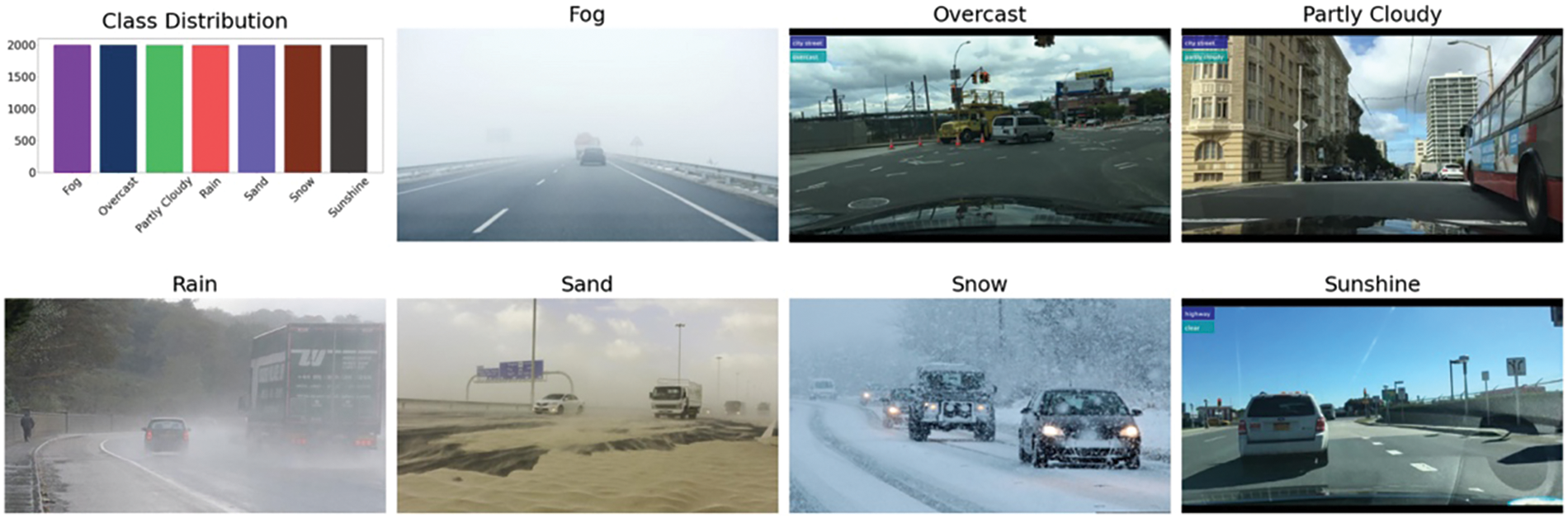
Figure 6: Class distribution of dataset and sample image from each class

2.6 Image Augmentation

Image augmentation techniques enhance training data diversity and variability, making models more robust and less sensitive to specific patterns or artifacts. They help prevent overfitting by exposing the model to a broader range of inputs, improving generalization. Using an Image Data Generator from TensorFlow [42], the original training data undergoes random transformations like rotations, shifts, flips, and zooms in each batch or epoch. Normalizing image pixels to the (0, 1) range ensures faster convergence and reduces training time. This process enriches training data without the need for manually creating or storing additional images, allowing the model to experience diverse augmented examples. Fig. 7 shows the data augmentation on an image from the fog class.

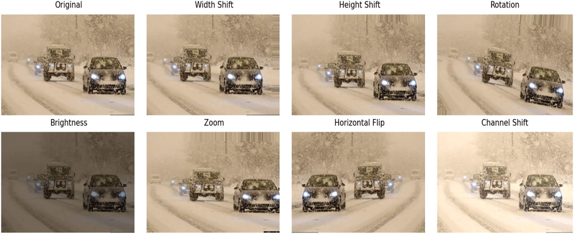
Figure 7: Image augmentation results on a single image from fog class

Empirical analysis shows that the following image augmentation techniques yield optimal results:

Rotation: Randomly rotates the image within a specified angle range, aiding in recognizing variations in object orientation.

Shifts: Includes width and height shifts (horizontally and vertically) and channel shifts (color intensity), mimicking displacement and color variations.

Brightness: Adjusts the overall brightness of an image.

Zoom: Randomly applies a zoom effect, simulating varying distances or scales of weather conditions.

Flips: Randomly flips the image horizontally.

3  Objectives, Outcome, and Interpretation

This section provides an overview of the experimental setup for the proposed work, detailing the environment in which the research was conducted. It covers the performance metrics utilized, optimization techniques employed during training, and the generated plots of the training progress. Also, the section presents the confusion matrices of the test data, which evaluate and assess the performance of the proposed work.

3.1 Experiment Environment

The test setup consists of a 13th Gen Intel Core i7-13620H CPU, NVIDIA GeForce RTX 4060 GPU (8 GB GDDR6), 32 GB RAM, running Windows 11, Python 3.10, and TensorFlow 2.12.

3.2 Key Performance Indicators (KPIs)

Metrics used to evaluate the performance of the developed model, such as Precision, Recall and F1-score.

3.3 Training R-MLKD

70% of the data is used for training, 15% for validation, and 15% for testing to evaluate model performance. The dataset is balanced across all seven classes.

a) Optimization Objective

In R-MLKD, KL divergence error ( measures the dissimilarity between two probability distributions, p and q. It is non-negative and equals zero when the distributions are identical. is an asymmetric measure, meaning that is not equal to ), making it useful for quantifying differences between distributions. between is defined in Eq. (5), where represent the kth elements of the and respectively.

(3)

Let and be the SoftMax probabilities with the Temperature of the first and second teacher networks and for the student network. With being the elements of the probability distributions of respective models, the distillation loss is defined in Eq. (4).

(4)

Here, is the number of samples in the batch. In this context, and are the SoftMax probabilities of the teacher and student, respectively.

Let , and represent the softened output probability distributions of the first teacher, second teacher and student models. They are obtained by applying the SoftMax function with a temperature T to the logits of the teacher and student models. Here, represents the indices of the probability distributions, i.e., the class probabilities. (••) the Kullback-Leibler (KL) divergence measures how one probability distribution diverges from a second, expected probability distribution. It measures the difference between each class’s teacher and student distributions in this context.

The distillation loss is the average KL divergence between the softened output distributions of the teachers and the student model. By minimizing this loss, the student model is encouraged to produce probability distributions similar to those of the teacher models, effectively “distilling” the knowledge from the teachers into the student. N1 is a normalization factor, where N represents the batch’s number of samples or data points. It ensures that the loss is averaged over all samples, providing a consistent scale for the loss regardless of the batch size.

The summation of the KL divergence terms indicates that both teacher models’ knowledge is considered. The student model is trained to mimic both teachers’ output distributions, combining their learned knowledge.

By substituting Eq. (4) into Eq. (3), we derive the student loss using KL divergence, resulting in Eq. (5). Eqs. (5) to (8) detail the distillation loss.

(5)

If we expand , we get Eq. (6).

(6)

By simplifying log terms in Eq. (6), we get Eq. (7).

(7)

Similarly, expanding and simplifying,

(8)

Minimizing the distillation loss helps the student model approximate the teacher models’ probabilities, effectively transferring their knowledge.

Temperature (T): Controls the softness or hardness of the probability distribution. A higher T results in softer probabilities, while a lower T results in more complex probabilities. T divides the networks’ SoftMax probabilities in the distillation loss equation before calculating KL divergence. The SoftMax function converts logits into probabilities, with its temperature-adjusted form defined in Eq. (9).

(9)

Here, represents the logits, and is the temperature parameter.

When T is greater than 1, the exponentiated values become smaller, making the differences between the output probabilities less pronounced, resulting in a “softer” probability distribution where the probabilities are more evenly spread across all classes. When T is less than 1, the exponentiated values become larger, especially for higher values of x. This amplifies the differences between the output probabilities, making the distribution “sharper” by increasing the probability for the most likely classes while reducing it for the others. When T = 1, the raw scores (logits) directly determine the output probabilities without any modification. A softer distribution (higher T) provides more information to the student model about the relative importance of all classes.

b) Overall Loss

The overall loss in R-MLKD combines distillation loss and student loss, weighted by hyperparameters, alpha and beta , where as defined in Eq. (10).

(10)

The weights and in the loss function were determined through manual tuning. Initially, equal weights were considered, and adjustments were made based on validation performance. A higher α was found beneficial for emphasizing the teacher outputs, particularly useful when dealing with limited or noisy labeled data. In contrast, a higher β was useful for focusing on the labeled data to prevent overfitting to the teachers’ outputs. The optimal balance was achieved by iteratively adjusting these weights to enhance the model’s performance on the validation set.

is the student loss based on the between the soft probabilities of the student network and the teacher networks and is calculated in Eq. (11).

(11)

is the training data. The weights balance the importance of distillation loss and student loss in the training objective, that is tuned for optimal knowledge transfer and learning. The primary objective is to reduce the overall loss.

c) Loss Function

KL divergence is used for both teachers and distillation, with details in Eq. (3). For final prediction, sparse categorical cross entropy loss measures the discrepancy between the predicted probabilities and true labels.

d) Regularization

BN, Dropout, and L2 Regularization are employed to improve model performance and prevent overfitting. In Batch Normalization, the inputs are normalized to have a standard distribution, aiding in faster convergence. Dropout works by randomly setting a fraction of input units to zero at each update during training, effectively preventing the model from over-relying on specific neurons. The input is multiplied by a binary mask generated from a Bernoulli distribution, which determines which units to drop.

L2 Regularization, also known as Weight Decay, adds a penalty term to the loss function, which helps reduce overfitting by minimizing the sum of the squared weights in the model. This ensures smoother gradients and prevents vanishing gradient problems. In the process, the regularization strength (λ) is set to 0.001, and the model parameters are adjusted based on the size of the training dataset.

e) Optimization Techniques

SGD with Momentum accelerates the convergence of standard SGD by incorporating momentum from previous updates. Instead of relying solely on the current gradient to update model parameters, it accumulates a moving average of past gradients, helping to navigate the optimization landscape more efficiently. This approach reduces oscillations and improves stability, especially in regions where the gradient direction changes frequently.

RMSprop adjusts the learning rate of each parameter individually based on a moving average of squared gradients, preventing drastic oscillations during updates. By maintaining an exponentially decaying average of the squared gradients, RMSprop stabilizes the learning process and improves convergence speed, especially in non-stationary or noisy environments.

f) Training Implementation

During training, the student loss function evaluates how closely the student’s predictions match the actual labels, while the distillation loss function measures the disparity between the softened predictions of the teachers and those of the student. The compile step configures the optimizer, metrics, student loss weight (alpha), Temperature (for softening probability distributions), and other hyperparameters. Callbacks, such as Model Checkpoint, customize training by saving the best model based on validation accuracy. Metrics monitor performance, and training continues across multiple epochs to enhance the replication of knowledge by the student.

The R-MLKD model was trained on a dataset comprising 1400 images (200 images per class). In Fig. 8, (a) and (b) depict accuracy and loss plots for ResNet50V2 (Teacher 1), achieving approximately 99.8% training accuracy and 96.2% validation accuracy, with respective losses of about 1.3% and 1.6%. Minor fluctuations of around 0.3% were observed, and using early stopping with a patience of 10, optimal performance was attained after 71 epochs. EfficientNetV2B3 (Teacher 2) exhibited similar trends, with training and validation accuracies near 99.9% and 97.4%, and losses around 1.7% and 1.8%, peaking at 61 epochs, 10 fewer than ResNet50V2. Training and validation losses were approximately 2.3% and 3.3%, respectively, with accuracy varying between 0.3% and 0.5%, and losses fluctuating between 0.7% and 1.5%.

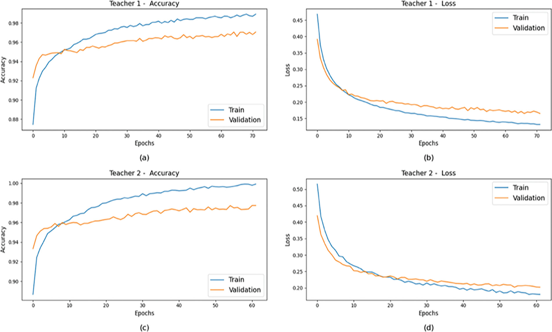
Figure 8: Comparison of Accuracy and Loss between training and validation data for (a) Accuracy of ResNet50V2, (b) Loss of ResNet50V2, (c) Accuracy of EfficientNetV2B3, (d) Loss of EfficientNetV2B3

Fig. 9a,b displays the training and validation accuracy of the student model, achieving 94.1% and 90.3%, respectively. As expected, when considered independently, the simple CNN model performed worse than the teacher models. However, through knowledge distillation from the teachers, as illustrated in Fig. 9c,d, the R-MLKD model achieved superior results with 99.9% training accuracy and 98.9% validation accuracy, alongside losses of around 0.1% and 0.2%. It reached its peak after 83 epochs, fewer than the standalone student model but more than the teacher models. Achieving high accuracy through knowledge distillation requires additional training epochs to strike a balance between epoch count and desired accuracy for optimal results.

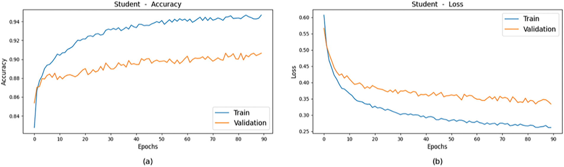
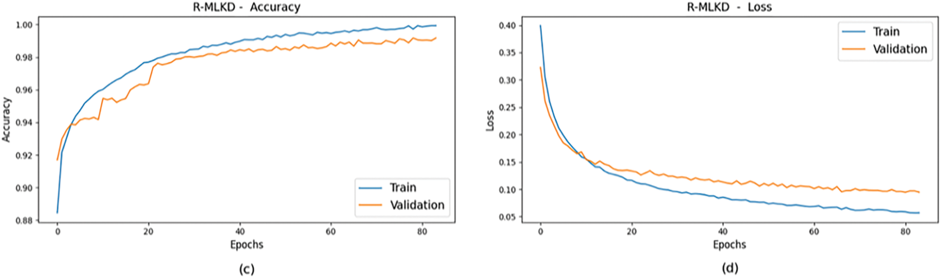
Figure 9: Comparison of Accuracy and Loss between training and validation data for (a) Accuracy Plot of Student, (b) Loss Plot of Student, (c) Accuracy Plot of R-MLKD, (d) Loss Plot of R-MLKD

The training and test procedure was carried out without data augmentation to determine the effect of data augmentation. The training accuracy showed no change, whereas the validation accuracy for Teacher 1 was 96.6% and for Teacher 2, 96.1%. The R-MLKD model’s validation accuracy was 97.2%. The results indicate the significant impact of data augmentation in improving performance. The results of the test dataset without data augmentation is provided in Table 1.

As approximated by the memory size, the model complexity is 89 MB for the ResNet50V2 teacher model and 69 MB for the EfficientNetV2B3 teacher model, while the student model (custom CNN) is 169 MB. The higher size of the student model is attributed to its architecture, which includes a significant number of trainable parameters optimized for feature extraction and classification tasks. In terms of computational load, the resource consumption (measured in GFLOPS) is 65.59 GFLOPS for ResNet50V2, 23.79 GFLOPS for EfficientNetV2B3, and 31.33 GFLOPS for the student model. Despite the custom CNN’s simpler architecture, it exhibits a relatively high GFLOPS, reflecting its capacity to effectively handle the distillation of knowledge from two complex teacher models. Regarding inference speed, the ResNet50V2 model typically requires 13 ms per image, and the EfficientNetV2B3 model requires 9 ms per image on a GPU. However, the MLKD framework student model achieves a competitive inference speed of approximately 17 ms per image on a GPU, making it suitable for practical applications that demand both efficiency and accuracy. This balance between model complexity, computational load, and inference speed highlights the effectiveness of our approach in practical engineering implementations.

3.4 Testing R-MLKD

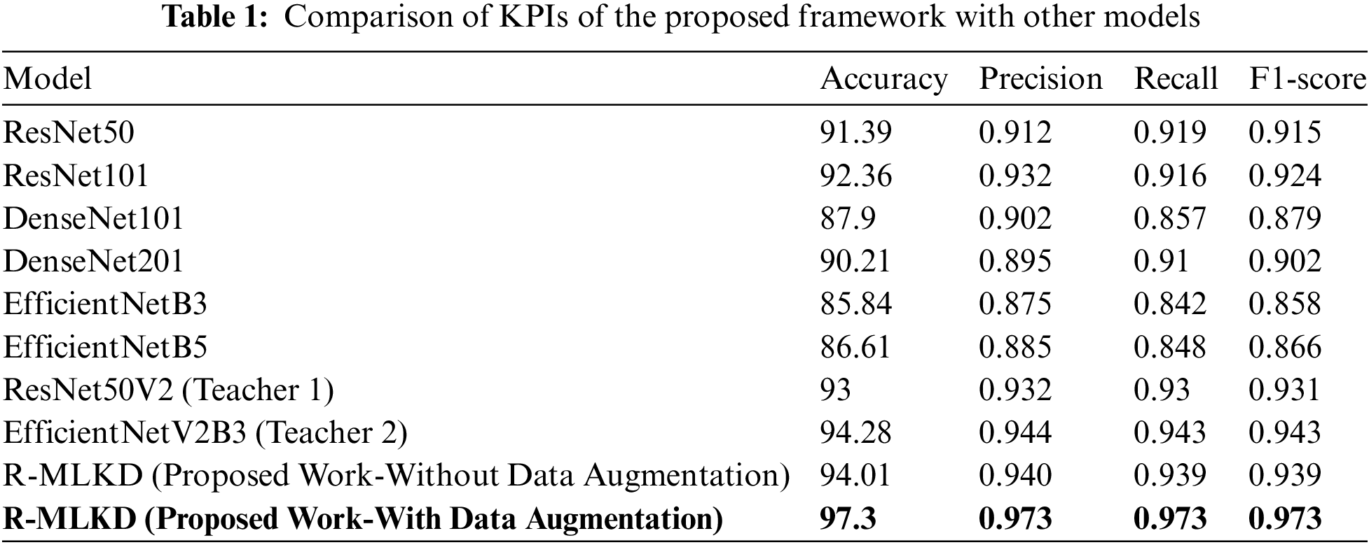
Table 1 presents key performance indicators (KPIs) evaluating teachers, students, and the R-MLKD model compared to other widely used CNN models. These include accuracy, precision, recall, and F1-score. The results indicate that the R-MLKD approach outperforms both individual teacher models and popular CNN variants. This demonstrates that multi-level knowledge distillation notably enhances weather condition classification for autonomous vehicles. Due to the utilization of a balanced dataset encompassing all seven classes, the metric values for each model are relatively consistent and comparable with R-MLKD, with about 3% higher accuracy than the EfficientNetV2B3 model.

4  Discussion

The proposed framework, R-MLKD, exhibits similarities to prior literature in its approach to detecting weather conditions for autonomous vehicles, particularly concerning the utilized datasets, learning policies, and development techniques. However, notable distinctions arise, particularly in the network architecture and the use of a balanced dataset. While the classification of weather conditions using key performance indicators and varying class numbers is explored in existing literature, a comparative analysis between our framework and state-of-the-art models would comprehensively assess our approach’s performance and effectiveness within the current research landscape.

Table 1 highlights the performance of various CNN models for weather condition classification in autonomous vehicles. The proposed R-MLKD model achieves the highest performance with 97.3% accuracy and precision, recall, and F1-scores of 0.973 each, significantly surpassing other models. Interestingly, the results of the R-MLKD model without data augmentation are still competitive, nearing the performance of EfficientNetV2B3. ResNet50 and ResNet101 show results with accuracies of 91.39% and 92.36%, respectively. DenseNet and EfficientNet models deliver respectable but lower accuracies. Teacher models, ResNet50V2 and EfficientNetV2B3 also perform well, with 93% and 94.28% accuracy, respectively. The computational complexity, resource consumption and the inference speed of each model are also calculated. The exceptional performance of the R-MLKD model highlights the substantial benefits of multi-level knowledge distillation, making it highly reliable for real-world applications like autonomous vehicle weather classification.

5  Conclusion

In this work, we have employed multi-level knowledge distillation, utilizing ResNet50V2 and EfficientNetV2B3 as teacher models and a custom CNN model as the student. The inclusion of ResNet50V2 and EfficientNetV2B3 as teacher models has proven advantageous, as these models possess deep architectures and have been pre-trained on large-scale datasets. They exhibit strong generalization capabilities and can effectively capture intricate details in weather condition images, making them well-suited for this classification task. Through the optimization and regularization techniques applied to the DAW, BDD100K, and CITS datasets, we have successfully achieved a remarkable F1-score of 0.973 in classifying weather conditions for autonomous vehicles. The results demonstrate the effectiveness of the proposed framework R-MLKD in accurately categorizing weather conditions.

Future work could incorporate temporal and multimodal data and enhance real-time performance for deployment in autonomous systems. Additionally, domain adaptation, self-supervised learning, and exploring hybrid distillation techniques can improve model generalization and scalability across diverse weather conditions while ensuring explainability for safer applications.

Acknowledgement: The authors would like to express appreciation to the MultiMedia University (MMU), Malaysia, SASTRA University, India and Garden City University, India for their technical and moral support.

Funding Statement: None.

Author Contributions: Jayakumar Chandrasekaran, Palaniyappan Sathyaprakash: Study Conception, Design, Data Collection; Bragadeesh Srinivasan Ananthanarayanan: Manuscript Preparation, Draft Preparation and Visualization; Parthasarathi Manivannan, Vaidhyashankar Jayakumar: Review of Results and Revision; Md Shohel Sayeed: Review of Results, Supervisor, Fund Acquisition. All authors reviewed the results and approved the final version of the manuscript.

Availability of Data and Materials: To validate the model, we used the following public datasets: Berkeley Deep Drive 100K (BDD100K) (10.1109/CVPR42600.2020.00271) (accessed on 05 August 2024); Diverse Aerial Weather Dataset (DAWN) (10.21227/bw1x-yh39) (accessed on 05 August 2024) and Connected Intelligent Transportation Systems (CITS) traffic alerts (https://doi.org/10.3390/s21041254) (accessed on 05 August 2024).

Ethics Approval: Not applicable.

Conflicts of Interest: The authors declare no conflicts of interest to report regarding the present study.

References

1. A. Biswas et al., “State-of-the-art review on recent advancements on lateral control of autonomous vehicles,” IEEE Access, vol. 10, pp. 114759–114786, 2022. doi: 10.1109/ACCESS.2022.3217213. [Google Scholar] [CrossRef]

2. J. Ondruš, E. Kolla, P. Vertaľ, and Ž. Šarić, “How do autonomous cars work?” Transp. Res. Procedia, vol. 44, no. 20, pp. 226–233, 2020. doi: 10.1016/j.trpro.2020.02.049. [Google Scholar] [CrossRef]

3. S. Singh and B. S. Saini, “Autonomous cars: Recent developments, challenges, and possible solutions,” IOP Conf. Ser. Mater. Sci. Eng., vol. 1022, no. 1, 2021, Art. no. 12028. doi: 10.1088/1757-899X/1022/1/012028. [Google Scholar] [CrossRef]

4. D. Parekh et al., “A review on autonomous vehicles: progress, methods and challenges,” Electronics, vol. 11, no. 14, 2022, Art. no. 2162. doi: 10.3390/electronics11142162. [Google Scholar] [CrossRef]

5. J. Vargas, S. Alsweiss, O. Toker, R. Razdan, and J. Santos, “An overview of autonomous vehicles sensors and their vulnerability to weather conditions,” Sensors, vol. 21, no. 16, 2021, Art. no. 5397. doi: 10.3390/s21165397. [Google Scholar] [PubMed] [CrossRef]

6. M. R. Bachute and J. M. Subhedar, “Autonomous driving architectures: Insights of machine learning and deep learning algorithms,” Mach. Learn. Appl., vol. 6, no. 8, 2021, Art. no. 100164. doi: 10.1016/j.mlwa.2021.100164. [Google Scholar] [CrossRef]

7. S. M. Mousavi, M. Zare, M. Ghorbani, and S. M. Moosavi, “A review of deep learning methods for weather image classification,” Sensors, vol. 21, no. 14, 2021, Art. no. 4735. doi: 10.3390/s21144735. [Google Scholar] [CrossRef]

8. K. He, X. Zhang, S. Ren, and J. Sun, “Deep residual learning for image recognition,” Comput. Vis. Pattern Recognit., 2016. doi: 10.48550/arXiv.1512.03385. [Google Scholar] [CrossRef]

9. M. Tan and Q. V. Le, “EfficientNet: Rethinking model scaling for convolutional neural networks,” in Proc. IEEE Conf. Mach.Learn. (ICML), Long Beach, CA, USA, 2019. doi: 10.48550/arXiv.1905.11946. [Google Scholar] [CrossRef]

10. K. K.Simonyan and A. Zisserman, “Very deep convolutional networks for large-scale image recognition,” 2014. doi: 10.48550/arXiv.1409.1556. [Google Scholar] [CrossRef]

11. J. Plested and T. Gedeon, “Deep transfer learning for image classification: A survey,” 2022. doi: 10.48550/arXiv.2205.09904. [Google Scholar] [CrossRef]

12. A. Mehra, M. Mandal, P. Narang, and V. Chamola, “ReViewNet: A fast and resource optimized network for enabling safe autonomous driving in hazy weather conditions,” IEEE Trans. Intell. Transp. Syst., vol. 22, no. 7, pp. 4256–4266, 2021. doi: 10.1109/TITS.2020.3013099. [Google Scholar] [CrossRef]

13. F. Yu, Z. Qin, C. Liu, D. Wang, and X. Chen, “REIN the RobuTS: Robust DNN-based image recognition in autonomous driving systems,” IEEE Trans. Comput. Aided Des. Integr. Circuits Syst., vol. 40, no. 6, pp. 1258–1271, 2021. doi: 10.1109/TCAD.2020.3033498. [Google Scholar] [CrossRef]

14. Q. A. Al-Haija, M. Gharaibeh, and A. Odeh, “Detection in adverse weather conditions for autonomous vehicles via deep learning,” AI, vol. 3, no. 2, pp. 303–317, 2022. doi: 10.3390/ai3020019. [Google Scholar] [CrossRef]

15. N. Arora, Y. Kumar, R. Karkra, and M. Kumar, “Automatic vehicle detection system in different environment conditions using fast R-CNN,” Multimed. Tools Appl., vol. 81, no. 13, pp. 18715–18735, 2022. doi: 10.1007/s11042-022-12347-8. [Google Scholar] [CrossRef]

16. X. Han, “Modified cascade RCNN based on contextual information for vehicle detection,” Sens. Imaging, vol. 22, no. 1, 2021, Art. no. 19. doi: 10.1007/s11220-021-00342-6. [Google Scholar] [CrossRef]

17. H. H.Xiao, F. Zhang, Z. Shen, K. Wu, and J. Zhang, “Classification of weather phenomenon from images by using deep convolutional neural network,” Earth Space Sci., vol. 8, no. 5, 2021, Art. no. e2020EA001604. doi: 10.1029/2020EA001604. [Google Scholar] [CrossRef]

18. V. Mușat, I. Fursa, P. Newman, F. Cuzzolin, and A. Bradley, “Multi-weather city: Adverse weather stacking for autonomous driving,” in 2021 IEEE/CVF Int. Conf. Comput. Vis. Workshops (ICCVW), Montreal, QC, Canada, 2021, pp. 2906–2915. doi: 10.1109/ICCVW54120.2021.00325. [Google Scholar] [CrossRef]

19. Y. Zhang, A. Carballo, H. Yang, and K. Takeda, “Perception and sensing for autonomous vehicles under adverse weather conditions: A survey,” ISPRS J. Photogramm. Remote Sens., vol. 196, no. 11, pp. 146–177, 2023. doi: 10.1016/j.isprsjprs.2022.12.021. [Google Scholar] [CrossRef]

20. M. Hassaballah, M. A. Kenk, K. Muhammad, and S. Minaee, “Vehicle detection and tracking in adverse weather using a deep learning framework,” IEEE Trans. Intell. Transp. Syst., vol. 22, no. 7, pp. 4230–4242, 2021. doi: 10.1109/TITS.2020.3014013. [Google Scholar] [CrossRef]

21. A. Gbeminiyi Oluwafemi and W. Zenghui, “Multi-class weather classification from still image using said ensemble method,” in 2019 South. Afr. Univ. Power Eng. Conf./Robotics Mechatronics/Pattern Recognit. Assoc. S. Afr. (SAUPEC/RobMech/PRASA), Bloemfontein, South Africa, 2019, pp. 135–140. doi: 10.1109/RoboMech.2019.8704783. [Google Scholar] [CrossRef]

22. M. R. Ibrahim, J. Haworth, and T. Cheng, “WeatherNet: Recognising weather and visual conditions from street-level images using deep residual learning,” ISPRS Int J. Geoinf., vol. 8, no. 12, 2019, Art. no. 549. doi: 10.3390/ijgi8120549. [Google Scholar] [CrossRef]

23. Y. Wang and Y. Li, “Research on multi-class weather classification algorithm based on multi-model fusion,” in 2020 IEEE 4th Inf. Technol. Netw. Electron. Autom. Control Conf. (ITNEC), Chongqing, China, 2020, pp. 2251–2255. doi: 10.1109/ITNEC48623.2020.9084786. [Google Scholar] [CrossRef]

24. J. Xia, D. Xuan, L. Tan, and L. Xing, “ResNet15: Weather recognition on traffic road with deep convolutional neural network,” Adv. Meteorol., vol. 2020, 2020. doi: 10.1155/2020/6972826. [Google Scholar] [CrossRef]

25. Q. A. Al-Haija, M. A. Smadi, and S. Zein-Sabatto, “Multi-class weather classification using ResNet-18 CNN for autonomous IoT and CPS applications,” in Proc. Int. Conf. Computat. Sci. Computat. Intell., CSCI 2020, Las Vegas, NV, USA, 2020, pp. 1586–1591. doi: 10.1109/CSCI51800.2020.00293. [Google Scholar] [CrossRef]

26. F. Tung and G. Mori, “Multi-level knowledge distillation for image classification,” 2019. doi: 10.48550/arXiv.1904.04998. [Google Scholar] [CrossRef]

27. J. Gou, L. Sun, B. Yu, S. Wan, W. Ou and Z. Yi, “Multilevel attention-based sample correlations for knowledge distillation,” IEEE Trans. Ind. Inform., vol. 19, no. 5, pp. 7099–7109, May 2023. doi: 10.1109/TII.2022.3209672. [Google Scholar] [CrossRef]

28. K. He, X. Zhang, S. Ren, and J. Sun, “Identity mappings in deep residual networks,” in Computer Vision–ECCV 2016. Cham: Springer, 2016, vol. 9908. doi:10.1007/978-3-319-46493-0_38. [Google Scholar] [CrossRef]

29. M. Tan and Q. V. Le, “EfficientNetV2: Smaller models and faster training,” in Proc. 38th Int. Conf. Mach. Learn., 2021, pp. 10096–10106. doi: 10.5555/3448030.3448192. [Google Scholar] [CrossRef]

30. S. Muksimova, S. Umirzakova, S. Mardieva, and Y. -I. Cho, “Enhancing medical image denoising with innovative teacher-student model-based approaches for precision diagnostics,” Sensors, vol. 23, no. 23, 2023, Art. no. 9502. doi: 10.3390/s23239502. [Google Scholar] [PubMed] [CrossRef]

31. K. Lee, S. Kim, and E. C. Lee, “Fast and accurate facial expression image classification and regression method based on knowledge distillation,” Appl. Sci., vol. 13, no. 11, 2023, Art. no. 6409. doi: 10.3390/app13116409. [Google Scholar] [CrossRef]

32. T. Akilan and K. M. Baalamurugan, “Automated weather forecasting and field monitoring using GRU-CNN model along with IoT to support precision agriculture,” Expert. Syst. Appl., vol. 249, no. 8, 2024, Art. no. 123468. doi: 10.1016/j.eswa.2024.123468. [Google Scholar] [CrossRef]

33. N. Reddy, M. Baktashmotlagh, and C. Arora, “Domain-Aware knowledge distillation for continual model generalization,” in 2024 IEEE/CVF Winter Conf. Appl. Comput. Vis. (WACV), Waikoloa, HI, USA, 2024, pp. 685–696. doi: 10.1109/WACV57701.2024.00075. [Google Scholar] [CrossRef]

34. T. -H. Le, S. -C. Huang, and Q. -V. Hoang, “Multi-level knowledge transmission for object detection in rainy night weather conditions,” IEEE Trans. Ind. Inform., vol. 20, no. 9, pp. 1–9, 2024. doi: 10.1109/TII.2024.3396552. [Google Scholar] [CrossRef]

35. F. Yu et al., “BDD100K: A diverse driving dataset for heterogeneous multitask learning,” in IEEE Conf. Comput. Vis. Pattern Recognit. (CVPR), Seattle, WA, USA, 2020, pp. 2633–2642. doi: 10.1109/CVPR42600.2020.00271. [Google Scholar] [CrossRef]

36. M. A. Kenk and M. Hassaballah, “DAWN: Vehicle detection in adverse weather nature,” in IEEE DataPort, 2020. doi: 10.21227/bw1x-yh39. [Google Scholar] [CrossRef]

37. O. Iparraguirre, A. Amundarain, A. Brazalez, and D. Borro, “Sensors on the move: Onboard camera-based real-time traffic alerts paving the way for cooperative roads,” Sensors, vol. 21, no. 4, 2021, Art. no. 1254. doi: 10.3390/s21041254. [Google Scholar] [PubMed] [CrossRef]

38. S. Ioffe and C. Szegedy, “Batch normalization: Accelerating deep network training by reducing internal covariate shift,” in Proc. 32nd Int. Conf. Mach. Learn. PMLR, Lille, France, 2015, vol. 37, pp. 448–456, 2015. [Google Scholar]

39. H. Alhichri, A. S. Alswayed, Y. Bazi, N. Ammour, and N. A. Alajlan, “Classification of remote sensing images using EfficientNet-B3 CNN model with attention,” IEEE Access, vol. 9, pp. 14078–14094, 2021. doi: 10.1109/ACCESS.2021.3051085. [Google Scholar] [CrossRef]

40. S. Kullback and R. A. Leibler, “On information and sufficiency,” Ann. Math. Statistics, vol. 22, no. 1, pp. 79–86, 1951. doi: 10.1214/aoms/1177729694. [Google Scholar] [CrossRef]

41. P. Gavrikov, “Visual keras,” GitHub repository, 2020. Accessed: Aug. 5, 2024. [Online]. Available: https://github.com/paulgavrikov/visualkeras [Google Scholar]

42. M. Abadi et al., “TensorFlow: Large-scale machine learning on heterogeneous systems,” 2015. doi: 10.48550/arXiv.1603.04467. [Google Scholar] [CrossRef]