Attribute Reduction on Decision Tables Based on Hausdorff Topology

1  Introduction

The rapid development of technologies in data collection and integration increases the complexity of data dimensions and noisy attributes [1,2]. Attribute reduction is indeed critical to selecting attributes according to the most significant contribution in the dataset [3,4]. Some applications of attribute reduction include data classification [1,2], and recommendation systems [5,6]. Recently, there have been some effective applications of RST in decision making support, including the diagnosis support in heart disease [7], COVID-19 (Corona Virus Disease 2019) [8], Chikungunya disease [9], Dengue fever [10] and data reduction [11]. From the original attribute set, attribute reduction aims to find out a subset that satisfies given constraints. Rough set theory (RST) is an effective tool for solving the attribute reduction problem for a long time [12–14]. RST-based attribute reduction methods often define a measure as the criteria for selecting the attributes. Some measures include fuzzy POS measure [15–17], intuitionistic fuzzy POS measure [18,19], fuzzy entropy measure [20–22], intuitionistic fuzzy entropy measure [23], fuzzy distance [24], intuitionistic fuzzy distance [25]. These measures are all based on approximate space for definition, so these approaches are expensive in storage and computation time.

Topological space is a powerful mathematical tool that is widely applied in many different areas of life [26–28]. The structure of a topology not only expresses the relationships among the objects in a set but also the relationships among the groups of objects in a set [29–31]. The reduct topology concept, proposed by Lashin et al. [29], grasped the attention of researchers in recent years [30,31]. Based on the mechanical similarity between rough sets and topologies [29], researchers have proposed many methods for building topologies according to the rough set approach, such as topology based on the RST covering approach [31], β-covering based rough sets [32], by the fuzzy rough set approach [33,34], by the intuitionistic fuzzy rough set approach [35,36] and by intuitionistic fuzzy approximate space [37]. The researchers also pointed out when the operations in the inner and outer regions of the topology are equivalent to the approximation operations of the rough set [38,39]. From the relationship between approximation operations of RST and topology, new RST models on topological space have been proposed [40]. The researchers also showed that the RST and topology are equivalent in the case of approximate space. Fig. 1 shows the approaches to attribute reduction in a decision table.

Figure 1: Attribute reduction approaches

Apart from the research on the relationship between rough set theory models and topologies, the methods used to build the Alexandrov topology structure regarding the rough set approach are also concerned and developed, including Alexandrov topologies based on the fuzzy rough set approach [33] and the intuitionistic fuzzy rough set approach [35].

Current attribute reduction methods based on algebraic topology approaches do not consider the separability of the attribute space. When separating attributes into non-intersecting groups, it will greatly reduce the number of candidate attribute sets that need to be processed. In this paper, we propose a Hausdorff topology structure using the RST approach to construct a novel attribute reduction method for decision tables. Unlike the structure of Alexandrov topologies, each element in a Hausdorff topology always has an opposite element, i.e., two different objects can be always distinguished through their neighbors. Then, we can use the Hausdorff topological structure as the standard structure for selecting the attributes. Furthermore, in 2014, Yun et al. [38] showed that two covers of attributes are different, but their topologies can be the same. Then, we can group attributes with the same topological structure. Based on those observations, a novel attribute reduction model, using the Hausdorff topology approach, is introduced. This model has the following main steps:

(1) Selecting: Filter attributes related to the reduct based on the criteria of Hausdorff’s proposed topological structure.

(2) Partitioning: Group the filtered attributes into groups based on the proposed co-structure concept. It should be noted that these groups of attributes do not intersect. Therefore, the number of groups will not be larger than the number of attributes obtained at the selection step.

(3) Wrapping: Wrapper the attribute groups obtained from the partitioning step to select the attribute group with the highest accuracy and consider this group as the reduct.

The main contributions of this paper include:

(1) Propose the Hausdorff topological structure based on the RST approach on the attribute space.

(2) Propose a novel attribute reduction method on topological space.

Apart from the introduction and conclusion sections, the paper’s structure includes: Section 2 recalls some basic knowledge of topology and rough sets. Section 3 proposes the method to construct a topology based on beta fuzzy approximation space. Section 4 studies the separability properties of the Hausdorff topology. Section 5 presents the attribute reduction model according to the Hausdorff topology structure. Section 6 presents some experimental results. The discussions are presented in Section 7.

2  Preliminaries

This section recalls some basic knowledge of RS and topology [29,38] that is essential background knowledge will be used in the next sections of this study.

The numeric decision table (shown in Table 1) is represented by the tuple DT=(U,C,D,f), where C∩D=∅, U is a non-empty set of objects, C is a non-empty set of conditional attributes, and D is a decision attribute. The function f determines a value for each u∈U corresponding to c∈C or D. For convenience, we denote DT=(U,C,D).

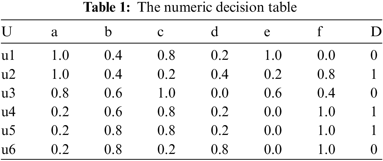
Definition 1. Given a decision table DT=(U,C,D) and an equivalence relation R on U. The pair (U,R) is an approximation space. Then the upper and lower approximation operations of X⊆U are defined by:

R_(X)={x∈U|[x]R⊆X}(1)

R¯(X)={x∈U|[x]R∩X≠∅}(2)

where [x]R is an equivalence class of x∈U according to the relation R or a subset of U that are the same with x according to the R. Then R_(X) is the set of objects in U that belong to X, and R¯(X) is the set of objects in U that could belong to X.

Definition 2. The topological space is defined as a pair (U,𝒯) consisting of a family of U subsets labelled 𝒯 that satisfy the following conditions:

(1)   ∅∈𝒯 and U∈𝒯;

(2)   𝒯 is closed under the finite intersection operation;

(3)   𝒯 is closed under any union operation.

Definition 3. Let R be an equivalence relation on U. Then R is a fuzzy equivalence relation if:

(1)   Reflexive: For all x∈U, R(x,x)=1;

(2)   Symmetric: For all x,y∈U, R(x,y)=R(y,x);

(3)   Min-transitive: For all x,y,z∈U, min(R(x,y),R(y,z))≤R(x,z).

Definition 4. Let R be a fuzzy equivalence relation on U, then R can be represented by the fuzzy equivalence relation matrix ℳ, where ℳ=[i,j]|U|×|U|.

Then, to get the lower approximation and the upper approximation of X⊆U, instead of using the approximation space (U,R) through the relation R, we can redefine the upper and lower approximation as follows:

ℳ_(X)={x∈U|M[x]⊆X}(3)

ℳ¯(X)={x∈U|M[x]∩X≠∅}(4)

Definition 5. Let 𝒜,ℬ be fuzzy equivalence relation matrices on U corresponding to A,B⊆C, then the intersection of two matrices is defined as follows:

𝒜[i,j]∩ℬ[i,j]=min(𝒜[i,j],ℬ[i,j]),∀i,j∈[1,|U|].(5)

Definition 6. Let 𝒜,ℬ be fuzzy equivalence relation matrices on U corresponding to A,B⊆C, then the union of two matrices is defined as follows:

𝒜[i,j]∪ℬ[i,j]=max(𝒜[i,j],ℬ[i,j]),∀i,j∈[1,|U|].(6)

Proposition 1. [38] Let ℳ be a relation matrix on U. For all X,Y⊆U

(1)   ℳ_(X)=(ℳ¯(Xc))c, ℳ¯(X)=(ℳ_(Xc))c where Xc=U∖X

(2)   ℳ_(U)=U, ℳ¯(∅)=∅

(3)   ℳ_(X∩Y)=ℳ_(X)∩ℳ_(Y), ℳ¯(X∪Y)=ℳ¯(X)∪ℳ¯(Y)

(4)   If X⊆Y then ℳ_(X)⊆ℳ_(Y), ℳ¯(X)⊆ℳ¯(Y)

(5)   ℳ_(X∪Y)⊇ℳ_(X)∪ℳ_(Y), ℳ¯(X∩Y)⊆ℳ¯(X)∩ℳ¯(Y)

Proposition 2. [38] Let ℳ be a relation matrix on U. For all X,Y⊆U

(1)   ℳ is serial if for any X⊆U: ℳ_(X)⊆ℳ¯(X) or ℳ¯(U)=U

(2)   ℳ is reflexive if for any X⊆U: ℳ_(X)⊆X or X⊆ℳ¯(U)

(3)   ℳ is symmetric if for any X⊆U: X⊆ℳ_(ℳ¯(X)) or ℳ¯(ℳ_(X))⊆X

(4)   ℳ is transitive if for any X⊆U: ℳ_(X)⊆ℳ_(ℳ_(X)) or X⊆U: ℳ¯(ℳ¯(X))⊆ℳ¯(X)

Proposition 3. [38] Let ℳ be a serial relation matrix on U. Then 𝒯={X⊆U|ℳ_(X)=ℳ¯(X)} is a topology on U.

3  Topologies Induced by β Fuzzy Approximation

Based on the fundamental knowledge presented in Section 2, in this section, we will discuss how to construct the topology from the β fuzzy approximation space. On that basis, we construct the algebraic structure of the proposed topology. We first define the concepts of β fuzzy equivalence relation, β fuzzy approximation space as below:

Definition 7. Let U be a non-empty set of objects in the interval [0, 1], the β fuzzy equivalence relation on U denoted by Rβ is defined as the following:

For all x,y∈U

Rβ(x,y)={1−|x−y|if1−|x−y|≥β0if1−|x−y|<β.(7)

Definition 8. Given DT=(U,C,D), the β fuzzy approximation space is denoted by (U,Rβ), where Rβ={Rβ(x,y)|x,y∈U}.

For each c∈C, we have U different values. We denote the relation Rβ with respect c∈C by Rcβ.

Definition 9. Given the decision table DT=(U,C,D) and ℳpβ, ℳqβ are β fuzzy equivalence relation matrices corresponding to Rpβ,Rqβ, p,q∈C. Then:

(1)   ℳpβ is less than (≺) ℳqβ if for all x,y∈U, Rpβ(x,y)<Rqβ(x,y);

(2)   ℳpβ=ℳqβ if for all x,y∈U then Rpβ(x,y)=Rqβ(x,y).

Proposition 4. Let (U,Rβ) be a fuzzy approximation space. Then 𝒯={X⊆U:Rβ_(X)=Rβ¯(X)} is a topology on U with respect Rβ.

Proof:

(1)   Based on the second property of Proposition 1, we have Rβ_(U)=U and Rβ¯(∅)=∅, then ∅∈𝒯 and U∈𝒯. This satisfies the first condition in Definition 2.

(2)   Assume that X,Y∈𝒯, then Rβ_(X)=Rβ¯(X), and Rβ_(Y)=Rβ¯(Y), and more Rβ_(X∩Y)⊆Rβ¯(X∩Y) and Rβ¯(X∩Y)⊆Rβ¯(X)∩Rβ¯(Y)=Rβ_(X)∩Rβ_(Y)=Rβ_(X∩Y). Then Rβ¯(X∩Y)=Rβ_(X∩Y). It follows that X∩Y∈𝒯. This satisfies the second condition in Definition 2.

(3)   Assume that Xk∈𝒯|k∈K. Then Rβ_(Xk)=Rβ¯(Xk), so for all k∈K, we have Rβ¯(∪k∈KXk)=∪k∈KRβ¯(Xk)=∪k∈KRβ_(Xk)⊆Rβ_(∪k∈KXk). In more Rβ_(∪k∈KXk)⊆Rβ¯(∪k∈KXk) so Rβ_(∪k∈KXk)=Rβ¯(∪k∈KXk). This satisfies the third condition in Definition 2.

From (1)–(3), we can conclude that 𝒯 is a topology on U with respect Rβ. ◻

Definition 10. Let DT=(U,C,D) and Raβ be a β fuzzy equivalence relation on U with respect a∈C. Then topology of the attribute a∈C denoted by 𝒯a is defined by:

𝒯a={X⊆U|Raβ_(X)=Raβ¯(X)}.(8)

Definition 11. Let 𝒯p,𝒯q be two topologies with respect Rpβ,Rqβ. Then 𝒯p⊆𝒯q if for all e∈𝒯p then e∈𝒯q.

Proposition 5. Let 𝒯p={X⊆U|Rpβ_(X)=Rpβ¯(X)} and 𝒯q={X⊆U|Rqβ_(X)=Rqβ¯(X)} be two topologies on U. Then 𝒯p⊆𝒯q if Rqβ≺Rpβ.

Proof:

Assume that Rpβ≺Rqβ, so for all x∈U we have [x]pβ⊆[x]qβ. Then for all X⊆U, if [x]qβ⊆X then [x]pβ⊆X, or in other words if X∈Tp then X∈Tq. Based on Definition 11, the Proposition has been proved. ◻

Definition 12. Let Rβ be a β fuzzy equivalence relation on U, then Rβ is the smoothest if and only if for all x,y∈U, Rβ(x,y)=1 if x=y and Rβ(x,y)=0 if x≠y. We denote the smoothest β fuzzy equivalence relation as R1β.

Proposition 6. 𝒯 is the largest topology (𝒯1) if Rβ=R1β.

Proof:

It is clear that the topology defined on R1β is the family S⊆U such that [x]1β⊆S. Furthermore, since [x]1β is the non-subset smallest of U then for all x∈U, the number of subset S⊆U such as [x]1β⊆S are |{2(U−x)}∪{x}|=|{2(U−x)}|=2|U−1|, that is the family of subset largest. The Proposition has been proved. ◻

Definition 13. Let Rβ be a β fuzzy equivalence relation on U, then Rβ is said to be coarsest relation if and only if for all x,y∈U, Rβ(x,y)=1. We denote the coarsest β fuzzy equivalence relation as R0β.

Proposition 7. 𝒯 is the smallest topology denoted by 𝒯0 if Rβ=R0β.

Proof:

It is clear that the topology defined on R0β is the family S⊆U such that [x]0β⊆S. Furthermore, since [x]0β=U is the non-subset largest of U then for all x∈U, the number of subset S⊆U such as [x]0β⊆S are |{2(U−x)}∪{U}|=|{U}|=1, that is the family of subset smallest. The Proposition has been proved. ◻

Definition 14. Let DT=(U,C,D) and R{p,q}β be a β fuzzy equivalence relation of p,q∈C on U, R{p,q}β=Rpβ∩Rqβ. Then topology on R{p,q}β is defined by:

𝒯{p,q}={X⊆U|R{p,q}β_(X)=R{p,q}β¯(X)}(9)

4  Hausdorff Topology from Topology Space

Based on the topological structure proposed in Section 3 of the article. In this section, we study the separability property of the Hausdorff topology. On that basis, we also examine the relationships of objects in U to determine in which cases 𝒯 is a Hausdorff topology on U.

Corollary 1. Given a topology 𝒯 base on Proposition 4. If X∈𝒯, then ∃Y∈𝒯:Y=U∖X.

Definition 14. Given a topology 𝒯 with respect toRβ. Then the topology 𝒯 is said to be Hausdorff topology if every x≠y∈U always exists two open sets Vx,Vy∈𝒯 such that Vx∩Vy=∅.

Proposition 8. Given a topology 𝒯 base on Proposition 4. If 𝒯 is non-trivial topology then 𝒯 is a Hausdorff topology.

Proof:

Assume that 𝒯 is non-trivial topology, which mean that 𝒯 is not an empty set. Then, based on Corollary 1, if X∈𝒯 then there always exists Y such that X∩Y=∅. The proposition is proven. ◻

Thus, 𝒯 is called Hausdorff topology if 𝒯 is not empty in relation Rβ. The next question is how to make a relation Rβ, so that 𝒯 is not empty.

Definition 15. Let DT=(U,C,D) and Rβ be a β fuzzy equivalence relation on U. Then topology 𝒯 with respect Rβ is non-trivial topology if for all x∈U, exists y≠x∈U such that [x]Rβ∩[y]Rβ=∅.

Proposition 9. Let Rβ be a β fuzzy equivalence relation on U. Ifx≠y∈U are two the smallest elements and |[x]Rβ∩[y]Rβ=∅ then topology 𝒯 with respect Rβ is non-trivial topology.

Proof:

(1)   Suppose x>y and [x]Rβ∩[y]Rβ=∅, then according to Eq. (7) we have Rβ(x,y)=0 or 1−|x−y|<β.

(2)   For all z∈U−{x,y}, if z>x then z>y, so 1−|z−y|<β then Rβ(z,y)=0.

From (1) and (2), we have ∀z∈U:z>x,[z]Rβ∩[y]Rβ=∅. The Proposition has been proved. ◻

5  Attribute Reduction Based on Hausdorff Topology Space

Based on the topological structure proposed by Hausdorff, in this section, we propose an attribute reduction model according to the Hausdroff topological approach. Differing from current attribute reduction models, the proposed model includes three stages. In the first stage, we remove redundant attributes based on the definition of redundant attributes in the Hausdorff topological approach. In this stage, only properties with Hausdorff topological structure (based on Lemma 1 and Definition 16) are selected. In the second stage, we group condition attributes with the same structure as the decision attribute D based on the concept of D-homomorphism (based on Definition 16 and Definition 17). The third stage is used to choose the best attribute group according to the method of wrapping the attribute groups. To illustrate these stages, the evaluation of the proposed algorithm and illustrative numerical examples are presented. Table 2 details the differences between the Hausdorff topology attribute reduction method and the traditional approach.

Lemma 1. Let PD be a partition of the decision attribute D and 𝒯 be a Hausdorff topology. Then for every X∈PD, there always exists Y∈𝒯 such that X∩Y≠∅.

Proof:

Based on Corollary 1 we have 𝒯≠∅. For all X∈PD, suppose that ∃G∈𝒯:G∩X=∅, based on Corollary 1 ∃∼G=U∖G∈𝒯:∼G∩X≠∅. ◻

Definition 16. Given a decision table DT=(U,C,D). Then c∈C is called a relative attribute if the topology of c on U is a Hausdorff topology.

Therefore, the attributes that have a Hausdorff topological structure are all attributes that control the decision set D, which is always contained in candidate reducts and is often called relative attributes. The above property can help us deliver an attribute filtering step that is effected in the attribute reduction model with a much more optimal computational cost than traditional attribute filtering methods. Next, to wrap relative attributes effectively, we define some concepts to optimize candidate reduct sets.

Definition 17. Given a decision table DT=(U,C,D) and Hβ is a family Hausdorff topology of C base on Rβ. Then p∈Hβ is called homomorphic with q∈Hβ if Rpβ=Rqβ.

Definition 18. Given a decision table DT=(U,C,D) and Hβ is a family Hausdorff topology of C base on Rβ. Then p∈Hβ is called D-homomorphic with q∈Hβ if RpDβ=RqDβ. Where RpDβ=Rpβ∩RDβ,RqDβ=Rqβ∩RDβ.

Based on Definitions 16, 17, and 18, we propose an attribute reduction model using the Hausdorff topology approach. The proposed model includes three main independent phases. 1) Filter phase for relative attributes, 2) Phase grouping relative attributes, and 3) Phase wrapper groups of relative attributes.

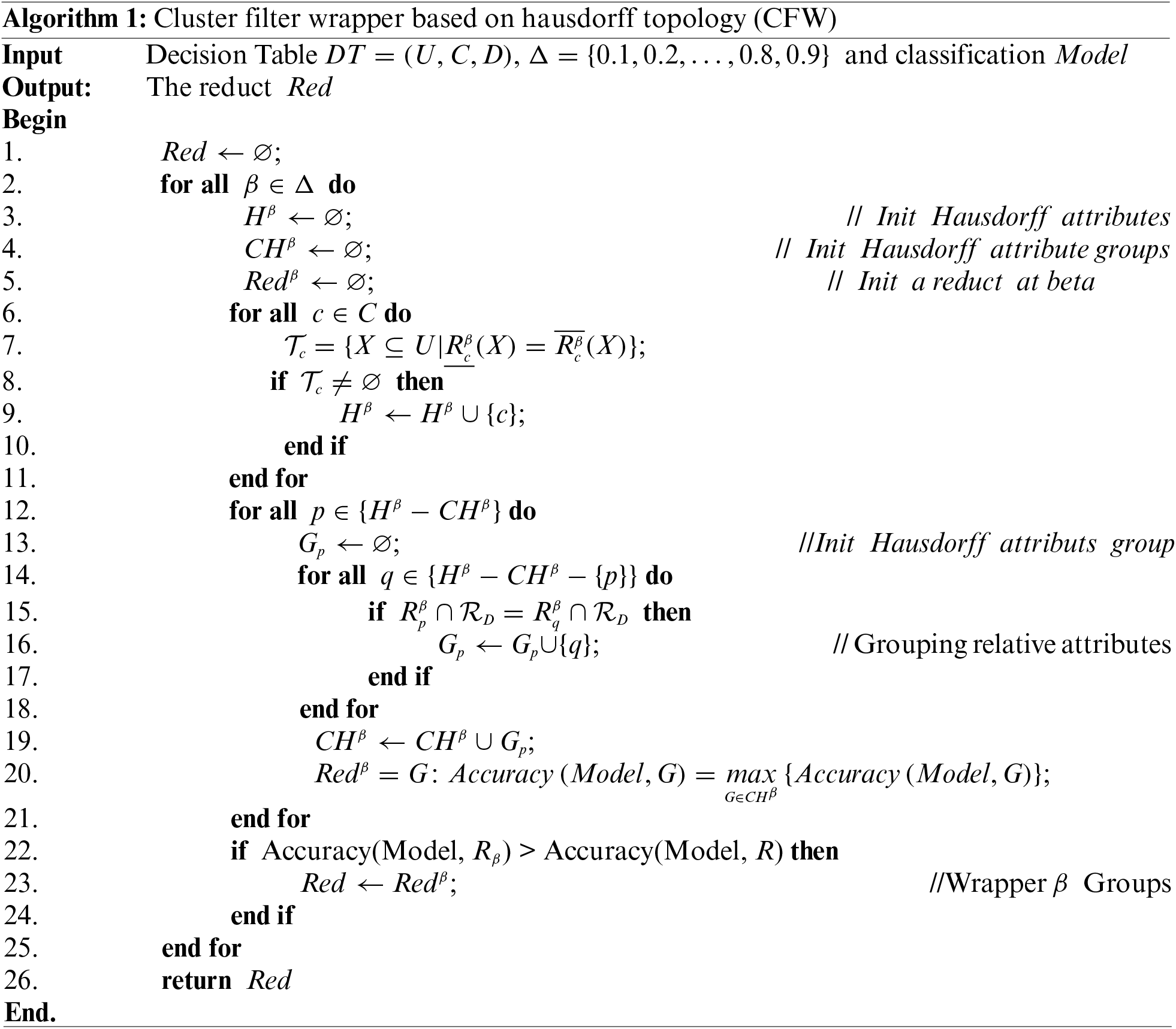
In this algorithm, we denote Hβ as Hausdorff attributes selected from the original attribute set C at β threshold. As mentioned, Hβ is a relative reduct set. CHβ are groups of attributes clustered from Hβ, where each item Gp in CHβ is a group of homomorphic attributes with attribute p. Therefore, the Hausdorff attribute wrapper phase is used to find the best reduct candidate at each β threshold. In reality, the Hausdorff attributes may not exist. Therefore, we use the threshold β in the threshold set Δ for adjustment. Then, for each value β, a different candidate reduct Redβ can exist. Therefore, the β wrapper stage determines the best candidate reduct for R. Next, we evaluate the complexity of the Algorithm 1 (CFW algorithm). Let |U| be the number of objects, |C| be the number of condition attributes, |Hβ| is the number of relative attributes, and |CHβ| is the number of groups of relative attributes. Then the complexity of 1) Steps 6–11 is 𝒪(2|U||C|); 2) Steps 14–18 is 𝒪(|U|2|Hβ|). Let T is the execution time of the Model classification, the complexity of Steps 20–22 is T. Then the complexity of Steps 12–21 is 𝒪(|U|2|Hβ|)+𝒪(|CHβ|T). With |Δ| is very small, from 1) and 2), we have the complexity of the algorithm is 𝒪(2|U||C|)+𝒪(|U|2|Hβ|)+𝒪(|CHβ|T). The details of CFW algorithm are presented in Fig. 2 below.

Figure 2: The diagram of the CFW algorithm

Fig. 2 shows the progress of the CFW algorithm. There are three stages in this algorithm. The first stage is performed to filter Hausdorff attributes Hβ from the attribute set C in decision table DT. In the second stage, a group of candidates CHβ is generated. In the last stage, the wrapper method is used in order to define Redβ where Redβ is the reduct with the highest accuracy among the candidates in CHβ. CFW algorithm stops when all values of beta in Δ are taken and the final reduct Red is found.

Example

Let DT=(U,C,D) as Table 1 and β=0.7 we have:

−   Initialization steps: Red←∅; Hβ←∅; CHβ←∅; Redβ←∅;

−   Filtering relative attributes:

1)   The attribute a∈C has u3=0.6≠u4=0.0 and [u3]Ra0.7=[0.80.81000][u4]Ra0.7=[0   0   0111]

2)   The attribute b∈C has u1=0.2≠u3=0.4 and [u1]Rb0.7=[1   1   0.80.80   0][u3]Rb0.7=[0.80.81   1   0.80.8]

3)   The attribute c∈C has u1=0.6≠u2=0.0 and [u1]Rc0.7=[100.8110][u2]Rc0.7=[010   001]

4)   The attribute d∈C has u1=0.4≠u3=0.2 and [u1]Rd0.7=[1   0.80.81   1   0][u3]Rd0.7=[0.80   1   0.80.80]

5)   The attribute e∈C has u2=0.2≠u4=0.0 and [u2]Re0.7=[01   00.80.80.8][u4]Re0.7=[00.801   1   1]

6)   The attribute f∈C has u2=0.2≠u4=0.0 and [u1]Rf0.7=[100000][u3]Rf0.7=[001000]

7)   Base one the Definition 15 and Proposition 9 show that, only {a,c,f} attributes are topology Hausdorff, so Hβ={a,c,f}

−   Group relative attributes:

1)   Calculating the relational matrices for attributes in Hβ according to Eq. (7) we have:

Ra0.7=[110.8000110.80000.80.81000000111000111000111];

Rc0.7=[100.81100100010.8010.80.80100.8110100.8110010001];

Rf0.7=[1000000100.80.80.800100000.8011100.8011100.80111];

RD=[101001010110101001010110010110101001].

2)   According to Definition 18 we have:

     Considering attribute a, we see Ra0.7∩RD=Rc0.7∩RD=[100.80000100000.801000000110000110000001]

Then Ga={a,c}, so CHβ=CHβ∪Ga={{a,c}}.

Gf={f}, so CH=CH∪Gf={{a,c},{f}}; Assuming the attribute group {a,c} has the highest classification accuracy on Model, we get Red0.7={a,c}. Suppose the candidate reduct at value β=0.7 is the candidate with the highest classification accuracy on Model. Then we obtain the reduct Red=Red0.7={a,c}.

The Hausdorff topology does not always exist for every fuzzy approximation space. Therefore, the beta value is used to change the smoothness of the fuzzy partitions. According to Propositions 5 and 6, we can see the relationship between the topology structure and the smoothness of the fuzzy partition. The smoother the fuzzy partition, the larger the size of the topology, which means the possibility of the Hausdorff topology appearing is greater. In the experiment, we set the step value to 0.1 to clarify the difference after each change in beta value.

6  Experiments

6.1 Experimental Scenarios

The goal to evaluate the algorithm’s performance when applied to real datasets and to be the basis for affirming the theoretical foundation we propose is entirely reasonable. The following is the experimental plan for the proposed algorithm. Step 1: Choose the best β value for the algorithm on each dataset. This experimental process aims to choose the most suitable β value for each dataset, where β is in the [0, 1] range with each step of 0.1. Step 2: Compare the proposed algorithm with other attribute reduction algorithms. After choosing the best beta value of the proposed algorithm for each dataset, compare the proposed algorithm with some attribute reduction algorithms: (1) Attribute reduction algorithm according to the rough set (VPRS) approach [41]; (2) Attribute reduction algorithm according to the fuzzy rough set (FRS) approach [42]; (3) Attribute reduction algorithm according to the fuzzy information entropy (IFE) approach [21]; (4) Attribute reduction algorithm according to the fuzzy distance (FD) approach [24].

Each algorithm experiments on 90% of randomly selected data from each dataset for evaluation. Perform this evaluation 10 times with Support Vector Machine classification (SVM) and k-Nearest Neighbors models (kNN, k=|D|) for finding the best reduct. Each model uses precision measurement and the 10-fold cross-validation method. The result of evaluating the classification accuracy of the reduct is the average accuracy (expressed as a percentage) of 10 different times. Before performing the attribute reduction algorithm, we standard all datasets to the range [0, 1]. We use Python for all algorithms on the Anaconda 3.6 platform running on a Windows 10 operating system with an i5 Processor and 8 GB of RAM (Random Access Memory). All algorithms were performed on 16 datasets from UCI [43].

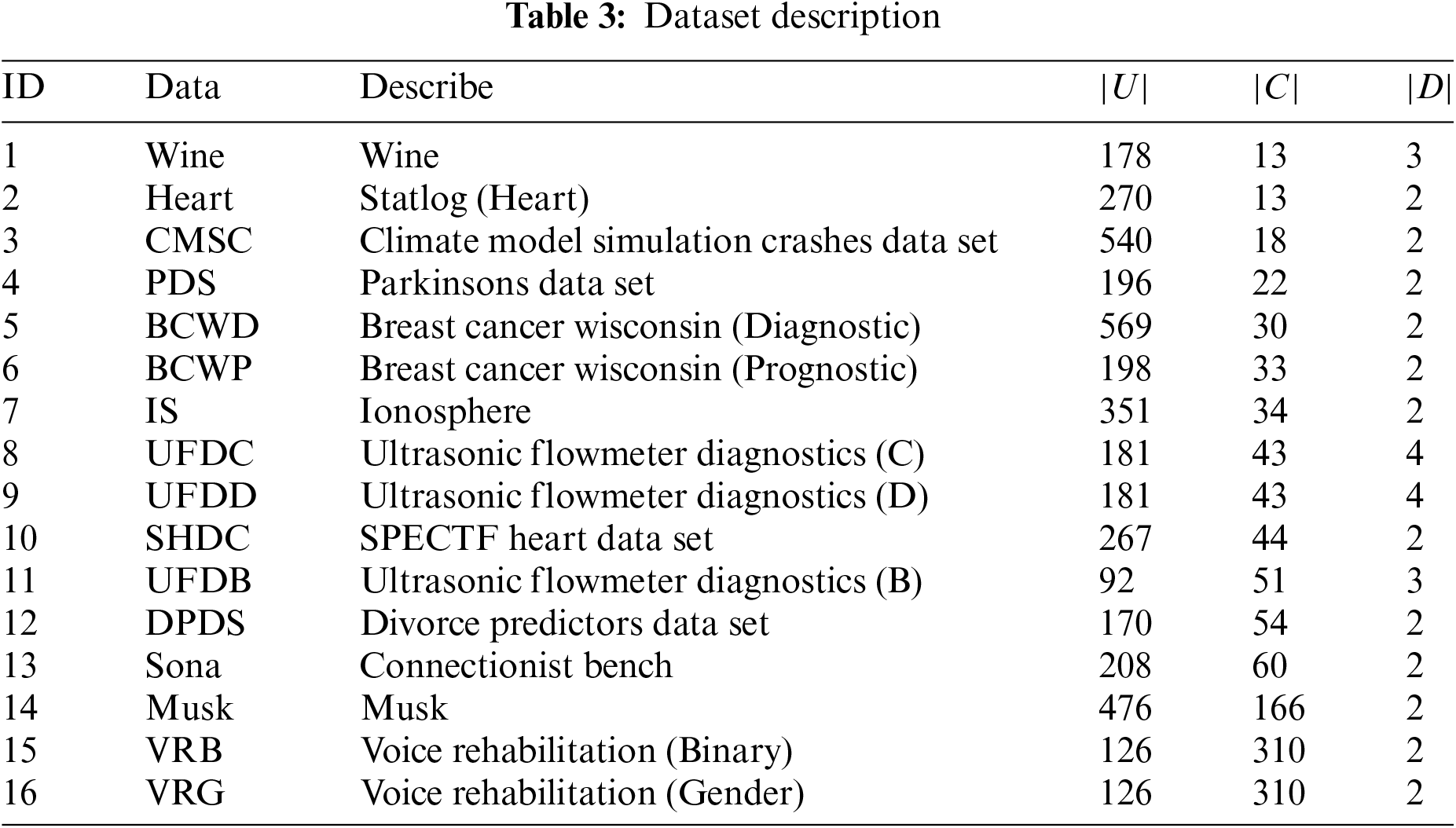
All the datasets are numeric data types. The details of the experimental data sets are in Table 3, with |U| as a sample number and |C| as the number of condition attributes arranged in ascending order. |D| as the class number of decision attributes. Especially in the UFDC and Sonar datasets that contain noise data, the model’s classification accuracy is low when used to train the model. Criteria to evaluate the effectiveness of algorithms include the computation time (in seconds), the size of the reduct (number of attributes), and classification accuracy (in percentage). Besides, the ability of the algorithms to handle noise is also considered.

6.2 Analysis the β Value for the Algorithm on Each Dataset

Before comparing the reduct with other algorithms, we need to find the β value such that the CFW algorithm gives the best reduct. For each experimental dataset, we perform the algorithm with different β values. We can get the best result for each β value in terms of size or classification accuracy. In this study, we choose the option that balances classification accuracy and the size of the reduct. The reduct obtained with the algorithms may differ for each classification model. Moreover, each β value may exist or not the reduct and these reducts have the size and classification accuracy different.

In Fig. 3, we can see the best β value for each dataset on the SVM classification model. Fig. 4 shows the best β value for each dataset on the kNN classification model. The results show that there is no linear relationship between the size and classification accuracy of the reduct with β, there is no linear relationship between the size and classification accuracy of the reduct.

Figure 3: The chart analyzes the relationship between the size and classification accuracy of the reduct at each specified value of β on the SVM classification model

Figure 4: The chart analyzes the relationship between the size and classification accuracy of the reduct at each specified value of β on the kNN classification model

Tables 4 and 5 describe the effects of the beta parameter on the size of the reduction, the classification accuracy and the running time of the CFW algorithm.

Table 4 shows the results of using SVM. Time consuming of CFW depends on the existence of reduct (|R| ≠ 0 or |R| = 0). When |R| = 0, it means that we cannot find the reduct by Topo Hausdorff approach or we cannot find the attributes satisfying Hausdorff properties by Definition 15 and Proposition 9. In this situation, the time consumption of the proposed algorithm equals zero. On selected datasets, the reducts are almost not defined when the beta is less than 0.5. When beta ≥0.5, the size of final reducts is different. The values of beta also affect the smoothness of partitions. The larger value of beta is, the higher the smooth in partitions is.

The results obtained by applying kNN are presented in Table 5 with similar characteristics as in Table 4.

From the results in Tables 4 and 5, the accuracy and size of reduct depend on the classification model applied in CFW algorithm.

6.3 Compare the Proposed Algorithm with Other Attribute Reduction Algorithms

After choosing β for the proposed algorithm, which has the best size and classification accuracy of the reduct. We compare the results of the proposed algorithm to other algorithms. Comparison standards include classification accuracy, the size of reducts, and the computation time. The average value of accuracy, the reduct’s size, and the computation time of the algorithms are denoted by |−|.

6.3.1 Evaluation of Algorithms on SVM Classification Model

The experimental results of the algorithms on the SVM classification model are presented in Tables 6, 7 and 9. Observing the results in the tables, we can see that the average classification accuracy on 16 datasets is not significantly different from the original dataset and the VPRS and FRS algorithms. However, the reduct’s size and the computation time are much better than the VPRS and FRS algorithms. The VPRS and FRS algorithms use the dependency measure according to the POS approach of the extended rough set model. The remaining IFE and FD algorithms using entropy and distance measures give the weakest average results regarding computation time and classification accuracy.

Fig. 5 explains the algorithms’ performance with the SVM classification model. Each figure illustrates the relationship between the reduct size and the classification ability of each algorithm on each dataset. We can see the difference in the reduct’s size from each algorithm and its classification accuracy. The proposed algorithm is superior in time to the other algorithms. The classification accuracy of the reduct from the algorithm method is also better on datasets Heart, CMC, PDS, BCWP, UFDC, SHDC, DPDS, Sonar, classification accuracy increased from 44% to 59% for noisy datasets UFDS, Sonar.

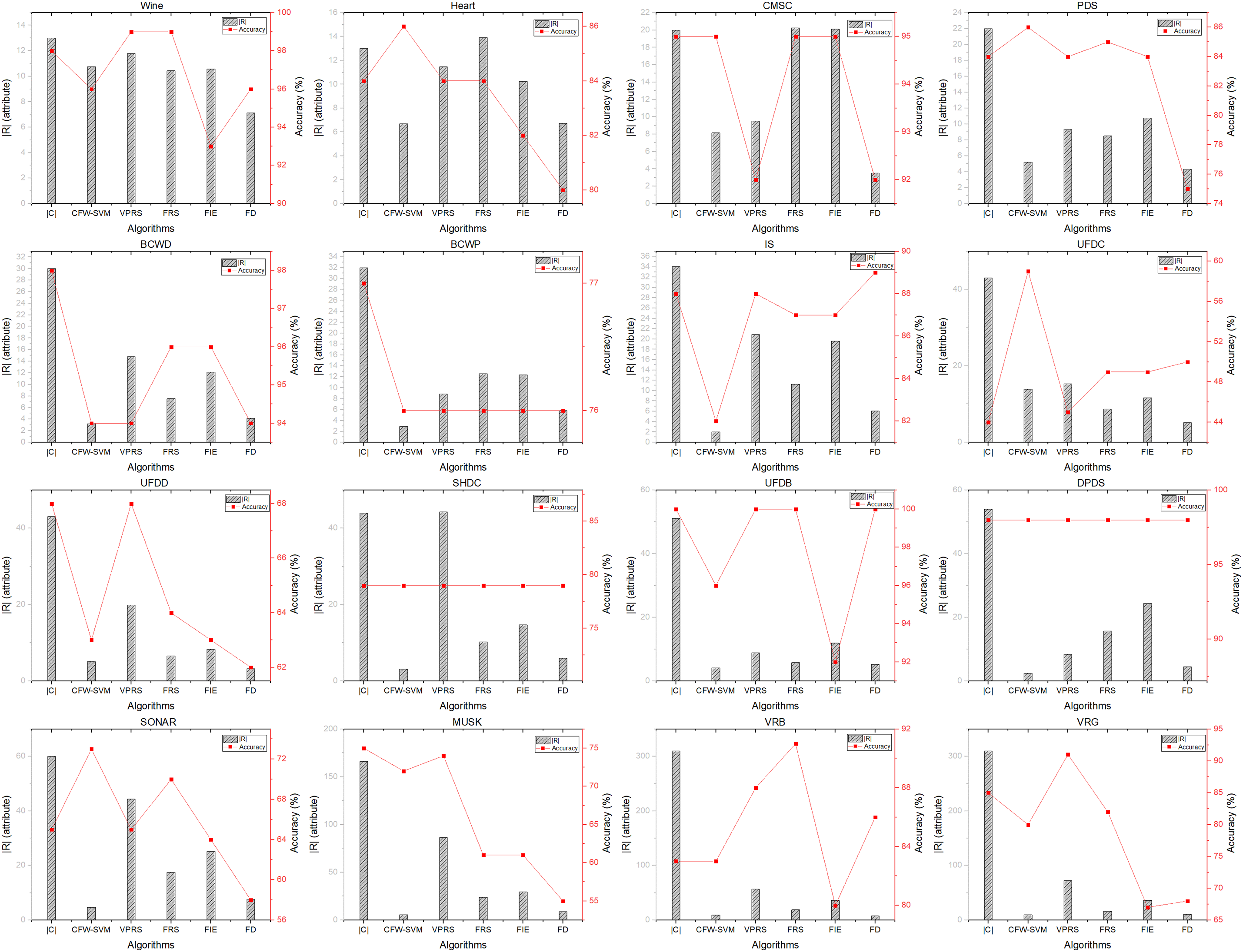
Figure 5: The diagram analyzes the relationship between the reduct’s size and classification accuracy at each algorithm on the SVM classification model

In general, on the SVM classification model, the proposed algorithm for the reduct is significantly better than the remaining algorithms, and the computation time is superior. Moreover, the proposed algorithm improves the classification accuracy for noise datasets.

6.3.2 Evaluation of Algorithms on kNN Classification Model

The experimental results of the kNN classification model of the algorithms are described in detail in Tables 6, 8 and 9. Observing the effects on each dataset with each evaluation criterion showed that 12 out of 16 datasets gave significantly better results than SVM classification model.

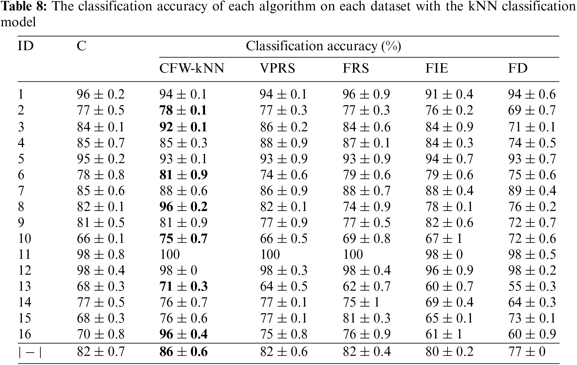
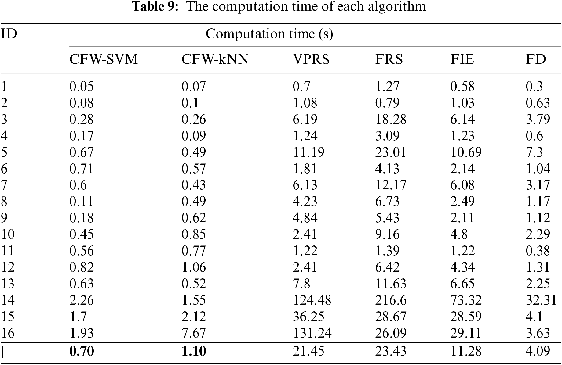
The remaining datasets have similar classification accuracy results, but the reduct’s size and computation time are superior. Fig. 6 provides an in-depth breakdown of the performance of several methods when applied to the kNN classification model. The scaler on each graph illustrates the relationship between the reduct’s size and the classification accuracy. We can notice the difference in classification accuracy and the difference in the reduct’s size achieved by each algorithm for each dataset. The proposed attribute reduction method is superior to the other algorithms.

Figure 6: The diagram analyzes the relationship between the reduct’s size and classification accuracy at each algorithm on the kNN classification model

In addition, the reduct from the proposed method has a higher level of accuracy Heart, CMCS, BCWP, IS, UFDC, UFDD, SHDC, UFDB, DPDS, Sonar, Musk, VRG. In particular, performance has been improved for the noise dataset VRG, with an improvement in accuracy from 70 to 96 percent.

In general, on the kNN classification model, the proposed algorithm for the reduct is significantly better than the remaining algorithms. In addition, the computation time and classification accuracy are superior to those of the compared algorithms that are depicted in Fig. 7.

Figure 7: The diagram analyzes the relationship between the computation time and |U| (left), between the computation time and |C| (right) of algorithms

7  Discussion

The experimental results presented in Section 6 of this study show that the proposed algorithm is superior to others. But the question is, what factors make the algorithm efficient regarding the computation time, the classification accuracy, and the reduct’s size? We will first analyze the computation time.

7.1 The Computation Time of the Proposed Algorithm

As presented in the introduction of this study, the proposed algorithm is significantly better than other algorithms in theoretical computation time. Most traditional attribute reduction methods use a filter with one-by-one attributes to create the reduct, which is ineffective for large-dimensional datasets.

Furthermore, traditional attribute reduction methods are based on granular computation, which has to use approximation spaces to process. Then, large datasets will have a significant computational load on this approximation space. Most of all have a complexity of 𝒪(|U|2|C|2). In contrast, the complexity of the proposed algorithm is 𝒪(2|U||C|)+𝒪(|U|2|Hβ|)+𝒪(|CHβ|T). Two special phases significantly improve the computation time, which the filtering phase of Hausdorff attributes with complexity is 𝒪(2|U||C|) and the cluster phase clustering the same structure Hausdorff attributes with complexity 𝒪(|U|2|Hβ|), where |Hβ| is much smaller than the original |C|. The effectiveness of time running of algorithms is presented in Fig. 7.

7.2 The Classification Accuracy of the Reduct from the Proposed Algorithm

Most of the traditional attribute reduction methods based on the rough set approach use the measure to evaluate the significance of the attribute. But those measures still have the disadvantage of only considering the similarity of two subsets based on the total components without considering the similarity for each element. Meanwhile, the topology approach allows us to evaluate the component’s similarity through the structure of that components. In this study, we use the Hausdorff topology structure because of distinguishable components in the Hausdorff topology. It is also why the traditional rough set model works so well on categorical datasets. So, we use the distinguishable concept in the rough set model for the topology space.

7.3 Size of the Reduct from the Proposed Algorithm

As mentioned above, the topology approach to distinguish attributes is better than the traditional approach. Yu et al. [38] have also shown that two different granular can have the same topology based on the rough set method. Therefore, the higher the similarity, the more attributes in the same group and vice versa. The attribute wrapper method is especially suitable for attribute reduction based on the topology approach. Suppose that the cluster phase divides the subset of the original attribute into many clusters. In that case, the resulting reduct will have a small size and a higher ability to choose a group of attributes with the best accuracy, and vice versa.

7.4 Two-Way ANOVA Analysis

After getting the experiment results from applying the proposed structure using 9 different values of beta in the range of [0, 1], two-way ANOVA (Analysis of Variance) is used in order to demonstrate the significance of the differences in performance metrics across various datasets. The significant level in this analysis is alpha = 0.05. Hypotheses, in this case, include Null hypothesis (H0): The means of accuracy on the datasets are the same. Alternative hypothesis (H1): There is at least one different value.

The summary results on kNN are presented in Table 10 below.

From two first rows in Table 10, the values of F are larger than F crit in both Values of beta and Datasets. This means that the different values of beta will lead to different levels of accuracy. Thus, in our experiments, the best value of beta is selected and applied to the topology. Moreover, the different datasets will get different values in accuracy.

The summary results of ANOVA analysis from applying SVM are presented in Table 11.

Due to the values of F being larger than F crit in both aspects in Table 11, we can state that by applying SVM in our topology, the different values of beta will lead to different levels of accuracy. Thus, the best value of beta is selected and applied to the topology.

8  Conclusion

As mentioned in the introduction, attribute reduction is an important problem widely applied in many fields related to knowledge processing. However, most current attribute reduction algorithms using the measure approach have the complexity of 𝒪(|U|2|C|2), so it is unsuitable for large datasets. The proposed method has a theoretical complexity of 𝒪(2|U||C|)+𝒪(|U|2|Hβ|)+𝒪(|CHβ|T) that much faster than the traditional attribute reduction method. The proposed algorithm is entirely new in both approach and design method, including:

1) Use the Hausdorff topology as a criterion to select relative attributes. This stage generates Hβ of relative reducts and has complexity 𝒪(2|U||C|), significantly improving the selection time of relative attributes.

2) Use the concept of dependent D-isomorphism to generate candidate reducts. This stage generates CHβ groups of candidate reducts that do not intersect and have complexity 𝒪(|U|2|Hβ|), significantly minimizing the number of candidate reducts.

In the future, we can develop new algorithms based on the distinguishing properties of Hausdorff topology, such as the cross-exchange method, cluster computation method, core computation method, dependent topological structure selection method, and some hybrid methods.

Acknowledgement: The authors are grateful to all the editors and anonymous reviewers for their comments and suggestions.

Funding Statement: This research is funded by Vietnam National Foundation for Science and Technology Development (NAFOSTED) under Grant Number 102.05-2021.10.

Author Contributions: Nguyen Long Giang and Le Hoang Son are responsible for idea convey and revised & review of the manuscript; Tran Thanh Dai is responsible for 1st draft writing and experiments; Tran Thi Ngan and Nguyen Nhu Son are responsible for data collection and preparation with analysis; Cu Nguyen Giap is responsible for all processes of research. All authors reviewed the results and approved the final version of the manuscript.

Availability of Data and Materials: Data is available from the corresponding author on reasonable request.

Ethics Approval: Not applicable.

Conflicts of Interest: The authors declare that they have no conflicts of interest to report regarding the present study.

References

1. S. Bashir, I. U. Khattak, A. Khan, F. H. Khan, A. Gani and M. Shiraz, “A novel feature selection method for classification of medical data using filters, wrappers, and embedded approaches,” Complexity, vol. 2022, no. 1, pp. 1–12, 2022. doi: 10.1155/2022/8190814. [Google Scholar] [CrossRef]

2. L. Meenachi and S. Ramakrishnan, “Differential evolution and ACO based global optimal feature selection with fuzzy rough set for cancer data classification,” Soft Comput., vol. 24, no. 24, pp. 18463–18475, 2020. doi: 10.1007/s00500-020-05070-9. [Google Scholar] [CrossRef]

3. M. Baldomero-Naranjo, L. I. Martínez-Merino, and A. M. Rodríguez-Chía, “A robust SVM-based approach with feature selection and outliers detection for classification problems,” Expert. Syst. Appl., vol. 178, no. 12, 2021, Art. no. 115017. doi: 10.1016/j.eswa.2021.115017. [Google Scholar] [CrossRef]

4. M. Riahi-Madvar, A. Akbari Azirani, B. Nasersharif, and B. Raahemi, “A new density-based subspace selection method using mutual information for high dimensional outlier detection,” Knowl.-Based Syst., vol. 216, no. 2, 2021. doi: 10.1016/j.knosys.2020.106733. [Google Scholar] [CrossRef]

5. A. J. Fernández-García, L. Iribarne, A. Corral, J. Criado, and J. Z. Wang, “A recommender system for component-based applications using machine learning techniques,” Knowl.-Based Syst., vol. 164, no. 4, pp. 68–84, 2019. doi: 10.1016/j.knosys.2018.10.019. [Google Scholar] [CrossRef]

6. B. Saravanan, V. Mohanraj, and J. Senthilkumar, “A fuzzy entropy technique for dimensionality reduction in recommender systems using deep learning,” Soft Comput., vol. 23, no. 8, pp. 2575–2583, 2019. doi: 10.1007/s00500-019-03807-9. [Google Scholar] [CrossRef]

7. D. I. Taher, R. Abu-Gdairi, M. K. El-Bably, and M. A. El-Gayar, “Decision-making in diagnosing heart failure problems using basic rough sets,” AIMS Math., vol. 9, no. 8, pp. 21816–21847, 2024. doi: 10.3934/math.20241061. [Google Scholar] [CrossRef]

8. R. Abu-Gdairi and M. K. El-Bably, “The accurate diagnosis for COVID-19 variants using nearly initial-rough sets,” Heliyon, vol. 10, no. 10, 2024, Art. no. e31288. doi: 10.1016/j.heliyon.2024.e31288. [Google Scholar] [PubMed] [CrossRef]

9. M. K. El-Bably, R. Abu-Gdairi, and M. A. El-Gayar, “Medical diagnosis for the problem of Chikungunya disease using soft rough sets,” AIMS Math., vol. 8, no. 4, pp. 9082–9105, 2023. doi: 10.3934/math.2023455. [Google Scholar] [CrossRef]

10. R. A. Hosny, R. Abu-Gdairi, and M. K. El-Bably, “Enhancing Dengue fever diagnosis with generalized rough sets: Utilizing initial-neighborhoods and ideals,” Alexandria Eng. J., vol. 94, no. 3, pp. 68–79, 2024. doi: 10.1016/j.aej.2024.03.028. [Google Scholar] [CrossRef]

11. R. Abu-Gdairi, A. A. El-Atik, and M. K. El-Bably, “Topological visualization and graph analysis of rough sets via neighborhoods: A medical application using human heart data,” AIMS Math., vol. 8, no. 11, pp. 26945–26967, 2023. doi: 10.3934/math.20231379. [Google Scholar] [CrossRef]

12. D. S. Truong, L. Thanh Hien, and N. Thanh Tung, “An effective algorithm for computing reducts in decision tables,” J. Comput. Sci. Cybern., vol. 38, no. 3, pp. 277–292, Sep. 2022. doi: 10.15625/1813-9663/38/3/17450. [Google Scholar] [CrossRef]

13. P. Viet Anh, V. Duc Thi, and N. Ngoc Cuong, “A novel algorithm for finding all reducts in the incomplete decision table,” J. Comput. Sci. Cybern., vol. 39, no. 4, pp. 313–321, Nov. 2023. doi: 10.15625/1813-9663/18680. [Google Scholar] [CrossRef]

14. P. M. Ngoc Ha, T. D. Tran, N. M. Hung, and H. T. Dung, “A novel extension method of VPFRS mode for attribute reduction problem in numerical decision tables,” J. Comput. Sci. Cybern., vol. 40, no. 1, pp. 37–51, Mar. 2024. doi: 10.15625/1813-9663/19696. [Google Scholar] [CrossRef]

15. J. Ye, J. Zhan, W. Ding, and H. Fujita, “A novel fuzzy rough set model with fuzzy neighborhood operators,” Inform. Sci., vol. 544, no. 1, pp. 266–297, 2021. doi: 10.1016/j.ins.2020.07.030. [Google Scholar] [CrossRef]

16. L. Zhang, J. Zhan, and J. C. R. Alcantud, “Novel classes of fuzzy soft β-coverings-based fuzzy rough sets with applications to multi-criteria fuzzy group decision making,” Soft Comput., vol. 23, no. 14, pp. 5327–5351, 2019. doi: 10.1007/s00500-018-3470-9. [Google Scholar] [CrossRef]

17. J. He, L. Qu, Z. Wang, Y. Chen, D. Luo and C. F. Wen, “Attribute reduction in an incomplete categorical decision information system based on fuzzy rough sets,” Artif. Intell. Rev., vol. 55, no. 7, pp. 5313–5348, 2022. doi: 10.1007/s10462-021-10117-w. [Google Scholar] [CrossRef]

18. X. Zhang, B. Zhou, and P. Li, “A general frame for intuitionistic fuzzy rough sets,” Inform. Sci., vol. 216, no. 5, pp. 34–49, 2012. doi: 10.1016/j.ins.2012.04.018. [Google Scholar] [CrossRef]

19. A. Tan, W. Z. Wu, Y. Qian, J. Liang, J. Chen and J. Li, “Intuitionistic fuzzy rough set-based granular structures and attribute subset selection,” IEEE Trans. Fuzzy Syst., vol. 27, no. 3, pp. 527–539, 2019. doi: 10.1109/TFUZZ.2018.2862870. [Google Scholar] [CrossRef]

20. Z. Li, Y. Chen, G. Zhang, L. Qu, and N. Xie, “Entropy measurement for a hybrid information system with images: An application in attribute reduction,” Soft Comput., vol. 26, no. 21, pp. 11243–11263, 2022. doi: 10.1007/s00500-022-07502-0. [Google Scholar] [CrossRef]

21. J. Xu, Y. Wang, H. Mu, and F. Huang, “Feature genes selection based on fuzzy neighborhood conditional entropy,” J. Intell. Fuzzy Syst., vol. 36, no. 1, pp. 117–126, 2019. doi: 10.3233/JIFS-18100. [Google Scholar] [CrossRef]

22. X. Ma, J. Wang, W. Yu, and Q. Zhang, “Attribute reduction of hybrid decision information systems based on fuzzy conditional information entropy,” Comput. Mater. Contin., vol. 79, no. 2, pp. 2063–2083, 2024. doi: 10.32604/cmc.2024.049147. [Google Scholar] [CrossRef]

23. A. Tan, S. Shi, W. Z. Wu, J. Li, and W. Pedrycz, “Granularity and entropy of intuitionistic fuzzy information and their applications,” IEEE Trans. Cybern., vol. 52, no. 1, pp. 192–204, 2022. doi: 10.1109/TCYB.2020.2973379. [Google Scholar] [PubMed] [CrossRef]

24. N. L. Giang et al., “Novel incremental algorithms for attribute reduction from dynamic decision tables using hybrid filter-wrapper with fuzzy partition distance,” IEEE Trans. Fuzzy Syst., vol. 28, no. 5, pp. 858–873, 2020. doi: 10.1109/TFUZZ.2019.2948586. [Google Scholar] [CrossRef]

25. T. T. Nguyen et al., “A novel filterwrapper algorithm on intuitionistic fuzzy set for attribute reduction from decision tables,” Int. J. Data Warehousing Min., vol. 17, no. 4, pp. 67–100, 2021. doi: 10.4018/IJDWM. [Google Scholar] [CrossRef]

26. S. E. Han, “Digital topological rough set structures and topological operators,” Topol. Appl., vol. 301, no. 2, 2021. doi: 10.1016/j.topol.2020.107507. [Google Scholar] [CrossRef]

27. S. Mishra and R. Srivastava, “Fuzzy topologies generated by fuzzy equivalence relations,” Soft Comput., vol. 22, no. 2, pp. 373–385, 2018. doi: 10.1007/s00500-016-2458-6. [Google Scholar] [CrossRef]

28. P. K. Singh and S. Tiwari, “Topological structures in rough set theory: A survey,” Hacettepe J. Math. Stat., vol. 49, no. 4, pp. 1270–1294, 2020. doi: 10.15672/hujms.662711. [Google Scholar] [CrossRef]

29. E. F. Lashin and T. Medhat, “Topological reduction of information systems,” Chaos Solitons Fractals, vol. 25, no. 2, pp. 277–286, 2005. doi: 10.1016/j.chaos.2004.09.107. [Google Scholar] [CrossRef]

30. Z. M. Ma and B. Q. Hu, “Topological and lattice structures of L-fuzzy rough sets determined by lower and upper sets,” Inform. Sci., vol. 218, no. 5, pp. 194–204, 2013. doi: 10.1016/j.ins.2012.06.029. [Google Scholar] [CrossRef]

31. L. Su and W. Zhu, “Dependence space of topology and its application to attribute reduction,” Int. J. Mach. Learn. Cybern., vol. 9, no. 4, pp. 691–698, 2018. doi: 10.1007/s13042-016-0598-8. [Google Scholar] [CrossRef]

32. S. E. Han, “Topological properties of locally finite covering rough sets and K-topological rough set structures,” Soft Comput., vol. 25, no. 10, pp. 6865–6877, 2021. doi: 10.1007/s00500-021-05693-6. [Google Scholar] [CrossRef]

33. C. Y. Wang, “Topological characterizations of generalized fuzzy rough sets,” Fuzzy Sets Syst., vol. 312, pp. 109–125, 2017. doi: 10.1016/j.fss.2016.02.005. [Google Scholar] [CrossRef]

34. K. Qin and Z. Pei, “On the topological properties of fuzzy rough sets,” Fuzzy Sets Syst., vol. 151, no. 3, pp. 601–613, 2005. doi: 10.1016/j.fss.2004.08.017. [Google Scholar] [CrossRef]

35. Z. Bashir, M. G. Abbas Malik, S. Asif, and T. Rashid, “The topological properties of intuitionistic fuzzy rough sets,” J. Intell. Fuzzy Syst., vol. 38, no. 1, pp. 795–807, 2020. doi: 10.3233/JIFS-179449. [Google Scholar] [CrossRef]

36. S. M. Yun, Y. S. Eom, and S. J. Lee, “Topology of the redefined intuitionistic fuzzy rough sets,” Int. J. Fuzzy Logic Intell. Syst., vol. 21, no. 4, pp. 369–377, 2021. doi: 10.5391/IJFIS.2021.21.4.369. [Google Scholar] [CrossRef]

37. T. T. Dai, N. L. Giang, V. D. Thi, T. T. Ngan, H. T. M. Chau and L. H. Son, “A new approach for attribute reduction from decision table based on intuitionistic fuzzy topology,” Soft Comput., vol. 28, no. 20, pp. 11799–11822, 2024. doi: 10.1007/s00500-024-09910-w. [Google Scholar] [CrossRef]

38. H. Yu and W. R. Zhan, “On the topological properties of generalized rough sets,” Inf. Sci., vol. 263, no. 1, pp. 141–152, 2014. doi: 10.1016/j.ins.2013.09.040. [Google Scholar] [CrossRef]

39. M. K. El-Bably, K. K. Fleifel, and O. A. Embaby, “Topological approaches to rough approximations based on closure operators,” Granul. Comput., vol. 7, no. 1, pp. 1–14, 2022. doi: 10.1007/s41066-020-00247-x. [Google Scholar] [CrossRef]

40. W. Yao and S. E. Han, “A topological approach to rough sets from a granular computing perspective,” Inf. Sci., vol. 627, no. 3–4, pp. 238–250, 2023. doi: 10.1016/j.ins.2023.02.020. [Google Scholar] [CrossRef]

41. S. Zhao, E. C. C. Tsang, and D. Chen, “The model of fuzzy variable precision rough sets,” IEEE Trans. Fuzzy Syst., vol. 17, no. 2, pp. 451–467, 2009. doi: 10.1109/TFUZZ.2009.2013204. [Google Scholar] [CrossRef]

42. R. Jensen and Q. Shen, “New approaches to fuzzy-rough feature selection,” IEEE Trans. Fuzzy Syst., vol. 17, no. 4, pp. 824–838, 2009. doi: 10.1109/TFUZZ.2008.924209. [Google Scholar] [CrossRef]

43. UCI, “Machine learning repository,” 2021. Accessed: Mar. 26, 2023. [Online]. Available: https://archive.ics.uci.edu/ml/index.php [Google Scholar]