Improved Double Deep Q Network Algorithm Based on Average Q-Value Estimation and Reward Redistribution for Robot Path Planning

1  Introduction

In the topic of autonomous navigation of mobile robots, path planning is a hot issue. Its goal is to search for a reliable and effective route from the initial location to the destination in an unknown environment without collision [1]. Initial conventional algorithms for path planning encompassed Rapidly-exploring Random Trees (RRT) algorithm [2], ant colony algorithm [3], A*algorithm [4], Dijkstrta algorithm [5], artificial potential field method [6] and genetic algorithm [7]. Nonetheless, the majority of these algorithms are based on previously established environmental knowledge. In actual environments, robots often cannot preemptively acquire all the environmental information. Therefore, how to achieve mobile robots perceive unknown environments and make autonomous decisions has evolved into a hot area of current research focus [8].

Compared to traditional path planning methods, the Reinforcement Learning (RL) based path planning algorithm enables mobile robots to autonomously learn about their environments and adapt to various complex and unknown situations [9]. Recently, an increasing number of studies have utilized RL in planning the trajectory of mobile robots and achieved fruitful results. Wen et al. [10] proposed a topological graph-based Multi-Sarsa algorithm, which adopts a two-level structure to improve the planning efficiency, in the first level the topological region is generated by dynamic growth of the region based on the grid graph, and in the second level the near-optimal paths are searched by using the two-level Multi-Sarsa algorithm, in which the first Q-table is initialized by the artificial potential field method to speed up the global path learning process, and the second Q-table is initialized by the connectivity domain of the topological map to optimize the local path planning. The combination of the two Q-tables realizes the synergy between the global and local levels. However, artificial potential field methods may oversimplify complex spatial relationships, and they rely heavily on predefined structures, which limits their ability to generalize in high-dimensional environments. Zhou et al. [11] proposed an improved version of the Q-learning algorithm, which uses root-mean-square (RMS) propagation to dynamically adjust the learning rate during the learning process, thus improving the path planning efficiency. However, the algorithm was only experimented in two-dimensional grids, and in more complex continuous spaces, the curse of dimensionality phenomenon occurs due to too many combinations of states and actions, resulting in the algorithm failing to converge. Although the RL based path planning algorithm has achieved lots of achievements in the domain of path planning for mobile robots, it is still difficult to deal with high-dimensional complex environments and dynamic environment changes.

Deep Reinforcement Learning (DRL) algorithms, through learning and optimization with deep neural networks, can discover more complex strategies, thereby finding better solutions and enhancing decision-making precision in intricate settings. In addition, DRL solves the problem that RL is prone to dimensional disasters when making real-time decisions in complex environments [12]. Based on the above advantages, DRL is now widely used in many fields, such as the rescue services [13], autonomous navigation [14], forest fire monitoring [15], smart agriculture [16], robot control [17] and so on. Especially in the robot path planning task, DRL plays a powerful advantage. Based on this, the purpose of this paper is to improve the efficiency and accuracy of robot path planning by studying the DDQN algorithm and improving the problems of sparse reward and low utilization of efficient data in the DDQN algorithm. Therefore, a DDQN algorithm based on average Q-value estimation and reward redistribution (AQRR-DDQN) was proposed. The major contributions of the paper are as follows:

(1)   To address the problem that there are large errors in the estimation of the target Q-value during the initial training phase, we proposed average Q-value estimation method, which involves averaging the previously learned K target Q-values to replace original Q-value.

(2)   The reward redistribution mechanism was designed. By dividing the final reward for each action into immediate rewards and discounted episodic rewards, the issue of low learning efficiency caused by sparse rewards can be addressed.

(3)   Introduced a reward-prioritized experience selection method to address the issue of high-quality sample loss in experience replay buffers by sorting the samples according to the reward value and controlling the extraction probability to increase the retention and utilization of high-quality experiences.

(4)   A comparative analysis was performed to evaluate the efficiency of the AQRR-DDQN algorithm by comparing it with other improved DDQN algorithms.

The subsequent sections of this article are structured thus: Section 2 presents related work. Section 3 introduces the implementation of the improved algorithm. In Section 4, perform simulation experiments and analyze the results. Section 5 puts forward summaries and prospects for the future work.

2  Related Works

By combining deep learning and reinforcement learning, DRL solves the problem that it is not feasible to use a table (such as Q-table) to store and update the value of each state-action pair due to the large state space, provides a powerful tool for solving complex decision problems, and promotes technological progress in many fields [18].

Since the introduction of DRL-based robotic path planning algorithms, many scholars have made lots of improvements. Li et al. [19] raised an enhanced DQN algorithm that assigns weights to stored samples and trains samples in priority order while removing highly similar sequences from the experience replay buffer to improve its efficiency. However, the algorithm is tested in a static and simple environment, and the algorithm lacks generalization ability. The problem of sparse reward for agents in complex environments is still not solved. Deguale et al. [20] introduced an adversarial DQN algorithm with reward modification and prioritized experience replay. The sparse reward problem is solved by redesigning the reward function to include obstacle avoidance and distance to the target location, and striking a balance between obstacle avoidance and moving towards the target. But the overestimation problem of DQN in estimating action values is still not solved, resulting in slow convergence of the algorithm. Zhao et al. [21] introduced a DQN algorithm reliant on time-sensitive reward mechanism, the collision information is skillfully incorporated into the rewards that are ultimately earned. This method alleviates the sparse reward problem prone to existing DQN algorithms. However, using the method of encoding individual nodes to describe the state of a discrete space is inefficient, which only applies to discrete spaces, and the computation time increases substantially as the complexity of the environment increases.

In order to solve the reward sparse problem and overestimation problem in DQN, various improved algorithms have been presented, especially for the DDQN algorithm [22]. DDQN alleviates the problem of overestimation by separating the process of action selection and Q-value estimation [23]. Therefore, a lot of studies about the robot path planning based on DDQN have been suggested, and some improvements have been made to improve the efficiency of the algorithm. Wang et al. [24] proposed an algorithm for dynamic path planning utilizing Tree DDQN, which optimized the tree structure by discarding the over-detected and unfinished paths. And combined the DDQN with the tree structure approach, multiple search paths are provided. However, the DDQN algorithm used in it adopted the way of experience replay to process experience samples, which may lead to some efficient data not being fully utilized. Jiang et al. [25] evaluated the current robot’s actions by using a second-order time difference approach, also the traditional experience pooling structure is replaced by a binary tree structure to store the results, which can effectively organize and store experience data to ensure that key and efficient data can be more utilized in the learning process. However, this also makes the computational complexity of the algorithm increase significantly, and the computational cost becomes higher. Yin et al. [26] proposed an adaptive operator selection paradigm based on the DDQN, which separates the Q-network into state value and action advantage networks. This design allows the algorithm to more frequently and accurately learn the state value function, thereby improving learning efficiency in multi-objective optimization tasks. However, the operator selection in this method is focused on historical rewards, which might limit its ability to fully balance exploration and exploitation when applied to complex optimization problems. Zhao et al. [27] put forward a DDQN algorithm combining optimal state classification and state splitting, which classifies, stores and processes multi-dimensional state information such as environment information and agent location information, thereby reducing the complexity of the state space and improving the convergence speed of the algorithm. But during the training process, the sampling of empirical samples is uniformly random, without prioritizing the samples according to their importance. This results in a low utilization of the efficient data. Peng et al. [28] proposed a Multistep DDQN algorithm (MS-DDQN) that combines the multistep update method with the DDQN algorithm. The multistep update method takes into account the cumulative reward over the next n steps and replaces the single-step Q-value update process in DDQN. This allows the algorithm to gather more information from longer-term rewards when faced with sparse rewards, thus avoiding the slow learning speed caused by sparse reward. Zhang et al. [29] put forward the idea of experience classification on the basis of MS-DDQN, proposed experience classification multi-step DDQN (ECMS-DDQN) algorithm. By classifying the experience samples and dynamically adjusting the sampling weight, the utilization efficiency of the obstacle-related experience samples is improved. However, the reliance on prior knowledge in experience classification makes the algorithm very sensitive to changes in the environment, limiting its generalization. Based on the inspiration of the above methods, an AQRR-DDQN algorithm is proposed to improve the sparse rewards problem and the utilization efficiency of experience sample. And the validity of the proposed algorithm is verified by comparing with MS-DDQN and ECMS-DDQN.

3  Theoretical Foundations

3.1 DDQN Algorithm

Deep neural networks serve as function approximators in the DQN algorithm to estimate the value function, which solves the problem of the dimensionality curse when there are too many states [30]. But the selection of actions is determined by the current network Q(s,a;θ), the Q-value with the optimal action is selected by max function in each iteration as the evaluation of the action. Due to the radical selection of actions, the overestimation problem may occur, while the DDQN conducts action selection and evaluation separately to alleviate the overestimation problem of Q-value [31].

First the Q-value contained every possible action is calculated through the current network Q(s,a;θ), and the argmax function is used to select the action corresponding to the maximum Q-value, as shown in Formula (1):

a′=arg maxa′Q(s′,a′;θ)(1)

In Formula (1), s′ is the new state reached after taking action a, a′ is the action chosen in the new state s′, θ is the parameter of the model.

Then actions in the target network Q^(s,a;θ′) is evaluated. The target Q-value is shown as Formula (2):

YDDQN=r+γQ^(s′,arg⁡maxa′Q(s′,a′;θ);θ′)(2)

In Formula (2), r represents the immediate reward for performing an action a, γ represents the discount factor used to adjust the weight of future rewards, θ′ represents the parameters of the target Q network.

During the training, a part of the sample is randomly selected from the experience replay buffer, the loss function is calculated by using the mean square error, and the network parameters are updated by the random gradient descent method. The updating process is shown in Formula (3):

L(θ)=E [(r+γQ^(s′,arg⁡maxa′Q(s′,a′;θ);θ′)−Q(s,a;θ))2](3)

The target value for updating parameters in the DDQN algorithm is shown as follows:

YDDQN={ris_done is truer+γQ^(s′,arg⁡maxa′Q(s′,a′;θ);θ′)is_done is false(4)

The only difference between the DQN and the DDQN algorithm lies in how the target Q-value is computed. DQN algorithm chooses the action that aligns with the highest Q-value within the target Q network and evaluates this action with the target Q network, while DDQN algorithm chooses the action that aligns with the highest Q-value within the Q network and evaluates this action with the target Q network. The detailed procedures for the DDQN algorithm are outlined as:

Step 1: Establish two same neural networks, designating one as the evaluation network and the other as the designated target Q network; initialize parameters, and set initial state s.

Step 2: The robot selects action a randomly based on the current action selection mechanism and executes a. And obtain new states s′ and immediate reward r from the environment.

Step 3: Store the state transition information (s,a,r,s′) in the experience replay buffer.

Step 4: Check whether the current number of steps is a multiple of the interval number C. If so, the Q network’s parameters are replicated onto the target Q network so that its parameters are regularly updated and synchronized, and then l samples (s,a,r,s′) are chosen at random for training from the experience buffer. If not, l samples (s,a,r,s′) are chosen at random straight for training from the experience buffer.

Step 5: Input the current state s from the state transition samples (s,a,r,s′) into the Q network. And input the next state s′ into the target Q network.

Step 6: The Q network not only outputs predicted future reward value but also calculates the Q-values for every possible action. Then, the argmax function serves to choose the action a′ that aligns with the maximum Q-value. The target Q network uses the action a′ selected by the Q network to calculate and output the target Q-value through Formula (4). Here, the action with the greatest Q-value is chosen by the Q network and the target Q network assesses this action, which mitigate the overestimation problem.

Step 7: Update Q network’s parameters by utilizing the network output values in Step 6.

Step 8: Next state s′ is used to replace the current state s. If s′ is the terminal state, end the learning process; otherwise, go back to Step 2.

3.2 Improved DDQN Algorithm

Compared with other algorithms, the DDQN algorithm has significant advantages in solving complex decision-making problems in path planning. This paper proposes an improved DDQN algorithm, which enhances the accuracy of target value estimation by accumulating and averaging multiple Q-values learned from target network instead of Q-value learned from a single target network. Additionally, a reward redistribution strategy is introduced to address the issue of sparse rewards, dividing the rewards into immediate and discounted episodic rewards to make the learning process more efficient. Also reward-prioritized experience selection method is proposed to improve traditional experience replay. The diagram of structure is shown in Fig. 1.

Figure 1: Schematic diagram of overall process

Among them, a neural network with a 4-layer DNN architecture is employed. The composition includes an output layer, an input layer, and two hidden layers. Two hidden layers contain 64 neurons and employ ReLU for its activation function. The 10 neurons in the input layer receive 10 input states from the agent. The output layer has 5 neurons and outputs the Q-values of 5 actions of the agent. The diagram of the model structure is shown in Fig. 2.

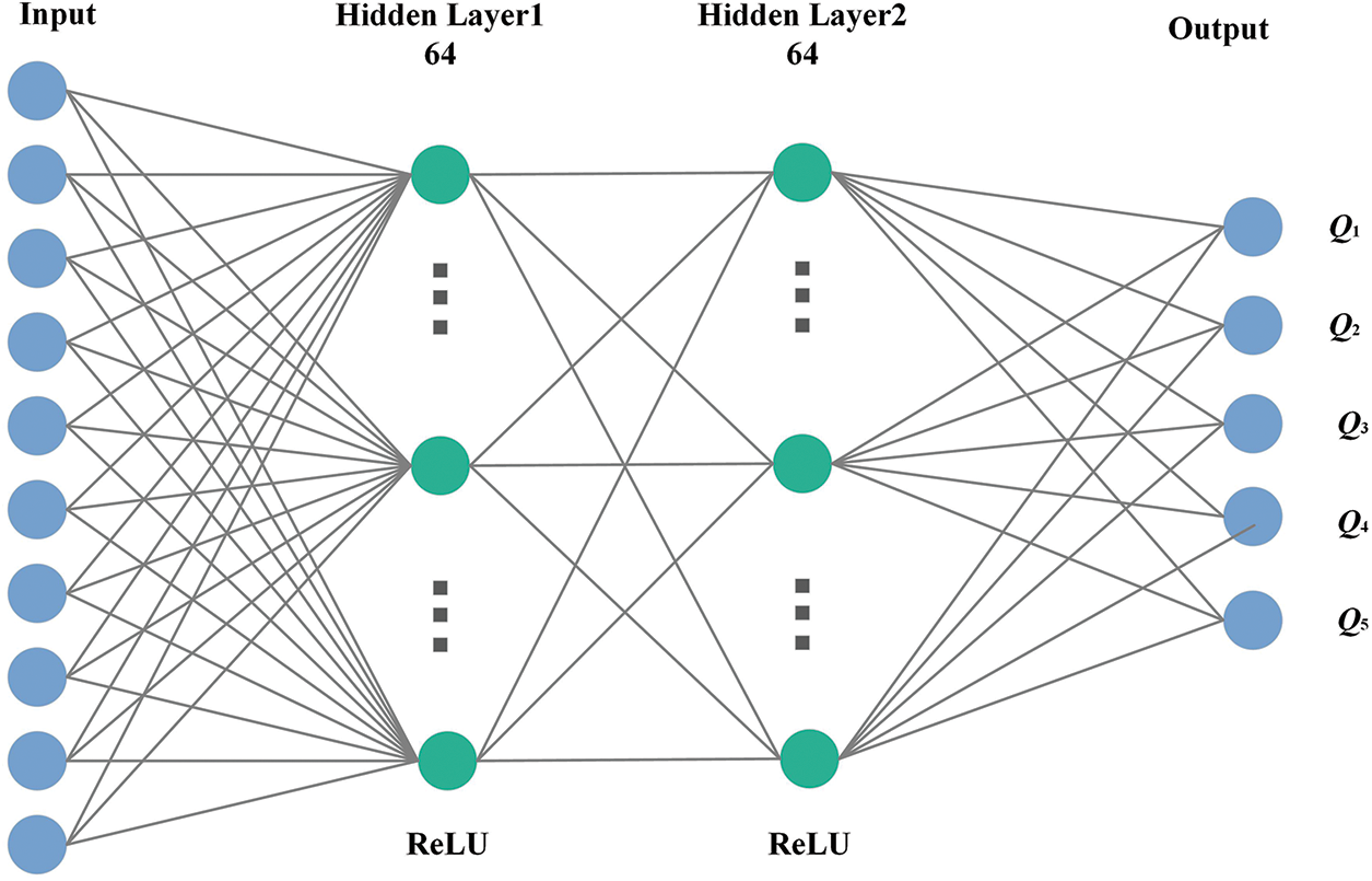
Figure 2: The diagram of neural network

3.2.1 Average Q-value Estimation Method

In the DDQN algorithm, the Q-value is obtained by target Q network learning. When the early network parameter deviation is large, there might also be a significant variation in the target Q-value, resulting in low training efficiency [32]. Based on the DDQN algorithm, this paper proposed an average Q-value estimation method. By averaging of K Q-values previously learned from the target Q network to replace the current Q-value, so as to reduce the error of target values. Equation can be represented as follows:

Q^TA(s,a)=1K∑k=1KQ^(s,a;θT−k)(5)

where Q^TA(s,a) represents the average value of the K Q-values of target Q network. K should be set in conjunction with the actual situation and application scenarios, and whether the setting is reasonable or not will directly affect the specific speed of training.

3.2.2 Reward Redistribution Mechanism

In RL, the robot relies on the reward function for action evaluation to complete the entire path search process [33]. Therefore, a reasonable reward function is important for the learning effect of agent. Collision behavior and the behavior of reaching the target position are the core factors for the robot to engage in environmental interactions. Considering only the core factors, the reward function can be designed as Formula (6):

rt={−r1collisionr2get_target0else(6)

where r1 and r2 are both positive numbers, The agent receives a reward of −r1 after a collision and a reward of r2 upon reaching the target. In this reward function, many actions receive a reward of 0, which does not accurately reflect the quality of all actions, making it difficult to effectively fit the optimal value function to the subsequent neural network. This paper introduced a reward redistribution mechanism, where the mobile robot receives different rewards for different actions. When the reward redistribution mechanism is used, the final reward for each behavior is divided into two parts: the immediate reward and the discounted round reward. Immediate reward is the reward value of the current action, and the discount round reward is expressed by a weighted sum of the reward values of future time steps, as shown in Formula (7):

Re(τ)=∑k=1T−tγkrt+k(7)

where t represents the current time step, T is the number of time steps required to complete an episode, Re(τ) represents the discount round reward from the current time step t to the end of the round time step T. γ is the discount factor. rt+k represents the reward at future time step t+k.

The final reward for each action is expressed by the sum of the immediate reward and the discount round reward, which can be expressed as Formula (8):

rt′=rt+Re(τ)(8)

where rt′ is the final reward value for each action, rt is the immediate reward of the current state. These rewards are applied to the neural network updates, thus enhancing its ability to more accurately align with the value function. The steps for how the reward redistribution applies to specific part of the DDQN are as follows:

(1) Calculation and assignment of rewards: the rewards are divided into two parts: immediate reward rt and discounted episodic reward Re(τ).

(2) Storage in the experience replay buffer: After each interaction with the environment, a tuple (s,a,rt,Re(τ),s′) is created and stored in the experience replay buffer.

(3) Calculation of the target Q-value (integration with DDQN): the target Q-value is calculated by combining the immediate reward and the discounted episodic reward as Formula (9):

Qtarget=rt+Re(τ)+γQ(s′,a′;θ)(9)

(4) Neural network update: The parameter of evaluation network is updated based on experiences sampled from the replay buffer. Then the loss is calculated using the mean squared error, and parameter θ is updated by gradient descent.

The reward redistribution mechanism, by combining immediate reward and discount round reward, enhances the accuracy of the target Q-value calculation, enabling the neural network to better align with the value function. But it also increases the computational complexity, especially in complex or dynamic environments. However, it can effectively improve the sparse reward problem and improve the learning efficiency of the algorithm, and the performance improvement brought by this mechanism is worth it in the long run.

3.2.3 Reward-Prioritized Experience Selection Method

In a traditional experience replay buffer, when it reaches maximum capacity, older experiences are discarded based on the first-in-first-out principle, which may result in high-reward experiences not being fully utilized. To address this issue, a reward-prioritized experience selection method is proposed. First, sample a set of experiences equal to or more than the batch size to form an expanded experience set Bextend. Then, Bextend is sorted based on reward values. From the sorted expanded experience set Bextend′, a certain proportion of high-reward experiences are selected, while the remaining samples are randomly selected from the rest to maintain exploration of the environment. The reward-prioritized experience selection method is illustrated in Fig. 3.

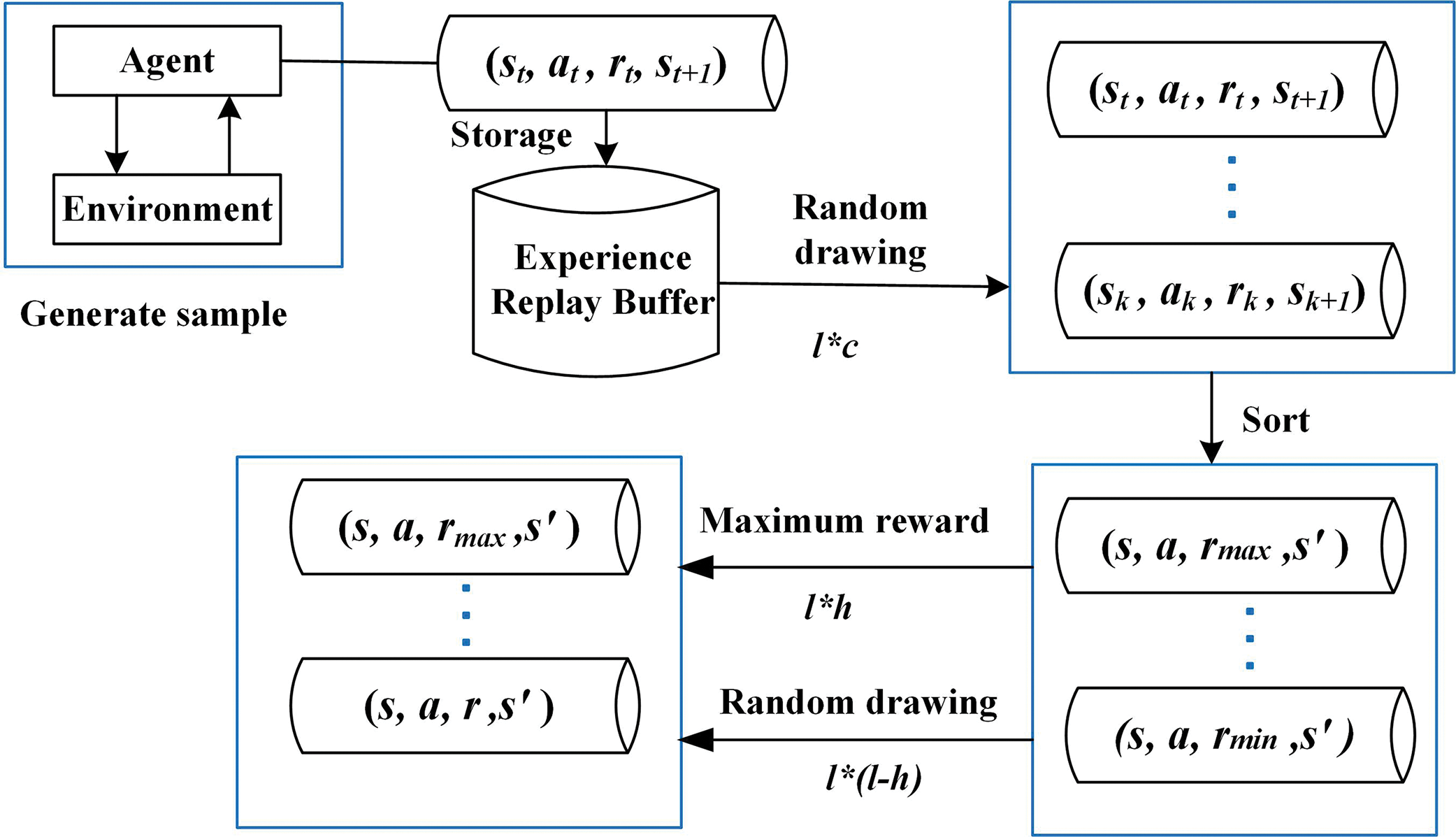
Figure 3: Schematic diagram of reward-prioritized experience selection method

The method sets two parameters: the expansion factor c and the selection probability h, which control the extent of new experience extraction and the proportion of high-reward experiences selected, respectively. The value range of the expansion coefficient c is c≥1, and l represents the count of samples used in batch gradient descent. The selection probability h determines the proportion of high-reward experiences selected from the sorted expanded set Bextend, with a value range of 0≤h≤1. This method ensures that high-reward samples are fully utilized while balancing the update of both high and low reward experiences in the buffer. It not only stops the algorithm from being trapped in local optimum, but also avoids the problems of overfitting.

3.2.4 Design of Improved DDQN Algorithm

When using DDQN algorithm to realize the path planning of robot, rewards are only obtained when agent encounters an obstacle or reaches the target position, leading to sparse rewards. Additionally, when the experience buffer reaches its maximum capacity, the first-in-first-out principle is executed, resulting in insufficient utilization of high-quality sample data. Therefore, based on the above improvements, Fig. 4 displays the flowchart for the improved algorithm, outlining the precise steps as follows:

Step 1: Establish two same neural networks, designating one as the Q network and the other as the designated target Q network; initialize parameters.

Step 2: Set the initial state s.

Step 3: Agent chooses and carries out an action a according to the current action selection mechanism, and gets the new state s′.

Step 4: Determine if the episode has ended. If the episode has not ended, obtain an immediate reward r; if the episode has ended, obtain both an immediate reward r and an episode reward Re(τ).

Step 5: Replace the current state s with the next state s, and go to Step 2.

Step 6: After the episode ends, recalculate the rewards for all actions in the episode using Formula (10) to get the final reward r′ for each action.

Step 7: Store the state transition information (s,a,r′,s′) into the experience buffer D.

Step 8: Randomly sample a batch of experiences Bextend of size l×c from the buffer D, sort them based on the reward values to form new experiences Bextend′. Then, select l×h experiences from Bextend′ in order of highest to lowest reward to store in the final experience set B. Finally, randomly select a size l×(1−h) of experiences from the remaining Bextend′ samples to add to the final experience set B.

Step 9: Input the current state s from the state transition sample (s,a,r′,s′) into the Q network, and input the next state s′ into the target Q network.

Step 10: The Q network outputs not only the predicted future return value but also calculates the Q-values for every possible action a, then selects the action a′ that aligns with the highest Q-value using the argmax function. Calculate the average Q-value using average Q-value estimation method. Finally, calculate the target Q-value by the average Q-value and the actions selected by the Q network.

Step 11: Update the parameters θ of Q network according to the network output value in Step 10. And the Q network’s parameters are sent to the target Q network every C steps.

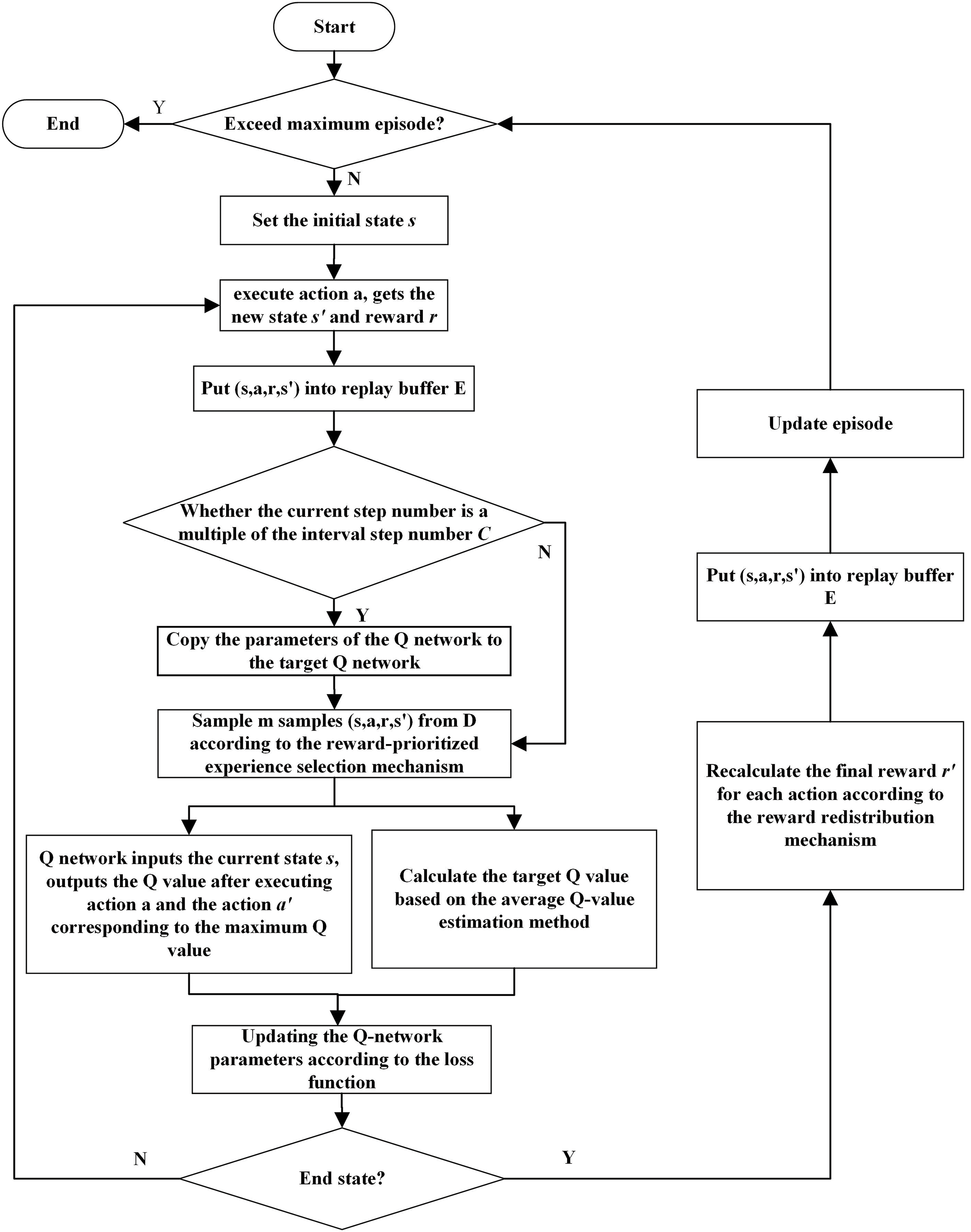
Figure 4: Algorithm flowchart

4  Simulation Results and Analyses

4.1 Design Experiment

(1) Simulation environment

The experimental operating system is Windows10. CPU is i5-8300H, 8 GB memory, 4 GB video memory. GPU is NVIDIA GeForce RTX 3060, CUDA 12.1, The version of Python used is 3.8, the versions of libraries employed during coding: numpy 1.24.4, pytorch 2.1.2, Matplotlib 3.7.4, gym 0.12.5, pickle, collections.deque, random. The CartPole-v1 environment provided by OpenAI Gym was used for testing. The actions of the agent are divided into: turn left 30°, turn left 15°, turn right 30°, turn right 15° and keep straight. The simulation environment is a square two-dimensional plane with a side length of 25 m, 5 to 7 obstacles are randomly generated in the environment. And the start and target positions are randomly generated.

(2) Reward function design

Reward is a kind of “reinforcement signal” provided by the environment in the process of path planning, which is an evaluation of every behavior. In order to improve the efficiency of the interaction between the agent and the environment and make it better use of the reward to adjust the action strategy, more detailed reward feedback is adopted in the design of the reward function. The reward value is debugged and validated several times in different scenarios.

1) When the direction changes, a reward of −0.01 points will be obtained.

2) When agent comes close to obstacles, a reward of −0.1 points will be obtained within a certain range of obstacle.

3) A reward of −1 points will be obtained when a collision occurs.

4) A final reward of 10 will be obtained when reaching the target position.

5) At each step, the agent receives a base reward of 10×Δdis, where Δdis represents the distance difference between two consecutive time steps, normalized by the diagonal length of the environment.

The specific reward function is as follows:

r={10×Δdisbase_reward−0.01direction_changed−0.1near_the_obstacles−1collision10reach_the_goal(10)

(3) Simulation parameters

According to the Reference [34], set εinit=0.99, εmin=0.01; according to the Reference [35] set the reward decay factor γ=0.6, set the learning rate α=0.001. Through several experiments and results comparison, set the update step interval C=100, average estimation coefficient K=5, expansion factor c=1.5, selection probability h=0.5. The maximum number of steps per episode Stepmax=1000, the maximum capacity of the experience replay buffer Mcapacity=20,000, the maximum number of iterations Tmax_episodes=100, the minimum exploration number Nexplore=500, and the batch size Nbatchsize=128. The parameters are shown in Table 1.

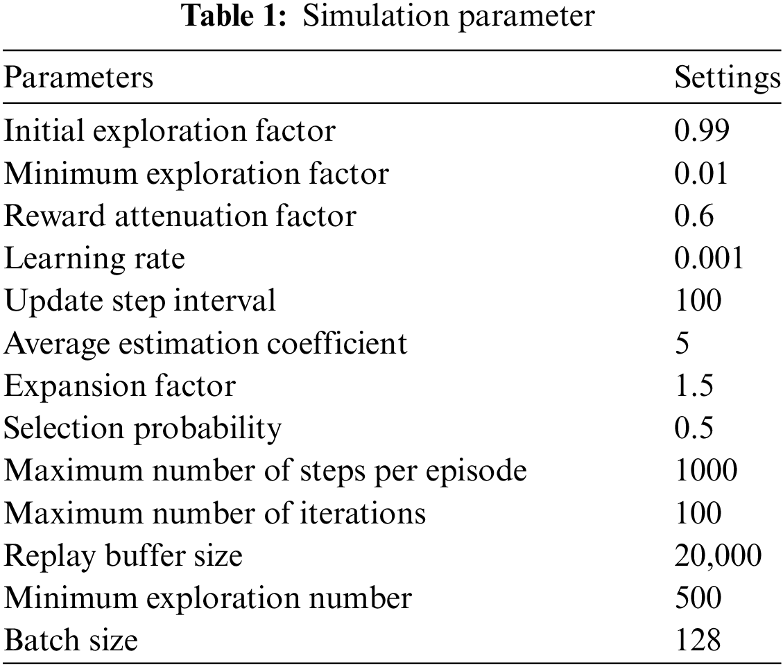
(4) Evaluation metrics

The four algorithms DDQN, MS-DDQN, ECMS-DDQN and AQRR-DDQN algorithm are trained respectively in fixed-position scenarios and random environments. Determine the algorithm performance based on the following indicators:

1) Total reward per episode: the higher the total reward, the better the algorithm performed at the task. It can be calculated as follows:

Rtotal=∑t=1Trt(11)

where rt is the reward at moment t, T is the total number of time steps in the round. Higher rewards indicate that the algorithm performs better in performing the task.

2) the average time taken: the time of agent reaches to target point, the calculation formula is:

Taverage=1N∑i=1NTi(12)

where Ti is the time for the intelligence to reach the target in the i-th round and N is the total number of rounds.

3) the average return value: the average of the total reward values every round. The higher the average return the more favorable it is for the intelligence to reach the target point. The calculation formula is as follows:

Raverage=1N∑i=1NRtotali(13)

4) the average number of steps: the average number of steps required by agent to complete the task in each episode. The lower the average number of steps, the shorter the path planned by agent. indicating higher efficiency. The calculation formula is as follows:

Saverage=1N∑i=1NSi(14)

where Si is the number of steps in the i-th round.

5) the average reward per step: the average reward value earned by agent at each time t. Higher average reward per step indicates that agent is more efficient and performs better. The calculation formula is as follows:

PRaverage=1N∑i=1NRtotaliSi(15)

4.2 Performance Simulation and Analyses

4.2.1 Test Result in Fixed Position Environment

The size of the experimental scene is a 25 m × 25 m planar continuous space, with five obstacles of fixed size and position, the yellow circle at the bottom left is the starting position, and the red circle at the top right indicates the target position. The visualization scene is shown in Fig. 5.

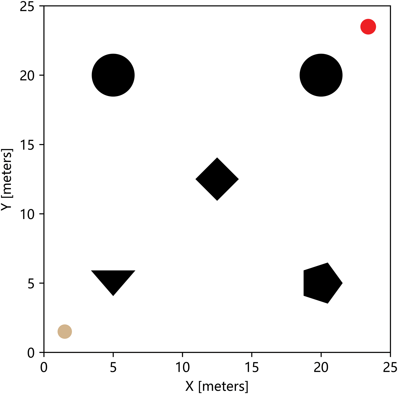
Figure 5: Fixed position environment

In the fixed position environment, by comparing the classical DDQN, MS-DDQN, ECMS-DDQN and AQRR-DDQN algorithm, it is evident that all four algorithms are able to plan a pathway to successfully get to the target location without collision at the end of training. And Fig. 6 displays the reward curves of the four algorithms, where the number of iterative episodes as the horizontal coordinate, and total rewards of each episode as the vertical coordinate.

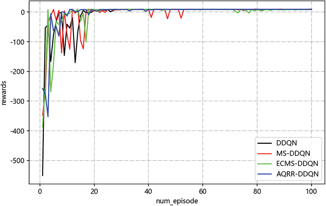
Figure 6: Comparison of return curves in fixed position environment

From Fig. 6, it can be seen that every algorithm is eventually able to converge, but there are clear differences in speed and stability. ECMS-DDQN algorithm shows the fastest initial rise in rewards, but fluctuates slightly in later stages, likely due to sensitivity to exploration-exploitation balance. The MS-DDQN algorithm also experiences fluctuations towards the end. In contrast, the AQRR-DDQN algorithm, though not the fastest initially, achieves the most stable performance with minimal fluctuations throughout the training. This stems from the improvement of the reward function, which introduces a reward redistribution mechanism to avoid the problem of sparse rewards, at the same time being less fluctuating and more stable than other algorithms in later training. With more consistent reward feedback, the agent was able to maintain a high level of strategic stability in the later stages of training. Fig. 7 shows the planned paths of the four algorithms after one training, in which blue, orange, green and red represent the paths of classical DDQN, MS-DDQN, ECMS-DDQN and AQRR-DDQN algorithm separately.

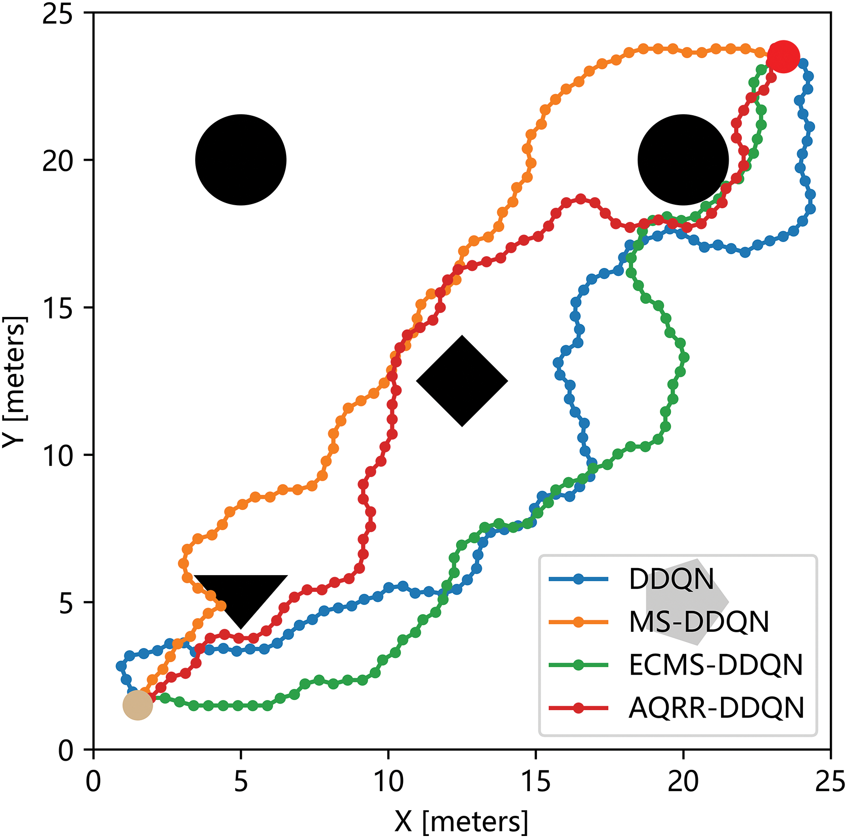
Figure 7: Comparison of optimal paths in fixed position environment

In Fig. 7, the DDQN algorithm appears to lack purposiveness, and although it can reach the target location, it is also convoluted and inefficient. Because the initial direction is detoured, ECMS-DDQN algorithm has been trying to adjust the direction. In the initial stage, MS-DDQN and the AQRR-DDQN algorithm choose to move directly towards the target position without going far around. When facing obstacles near the target position, the AQRR-DDQN algorithm chooses to adjust the direction and avoid approaching the obstacles. On the whole, the path given by the AQRR-DDQN algorithm has fewer turns, and the direction is adjusted in time when approaching obstacles to avoid collision with obstacles, which is relatively safe on the whole and does not have too much detour phenomenon.

Due to the randomness of the experiment, the relevant data of a single training may not be able to effectively show the performance differences of different algorithms. In this study, 100 times of path planning experiments were trained, and compare their performance. The items compared included the average time taken per algorithm, the average number of steps, the average reward per step and the average return value. The data for the last two comparison items were selected from the last 10 episodes of every training. The comparison results are displayed in Table 2.

Table 2 shows that the AQRR-DDQN algorithm has the shortest average time, which is about 61, 11 and 14 s less than the average time of DDQN, MS-DDQN and ECMS-DDQN algorithms, respectively. This improvement is closely related to the introduction of the average Q-estimation, which can accelerate the learning process by avoiding the policy bias caused by over-estimation of Q-value. AQRR-DDQN is the best in terms of the average number of steps, with an average of 89.103, which is significantly lower than other algorithms. This advantage can be attributed to the reward-prioritized experience selection, which reduces ineffective exploration by prioritizing the learning of high-value experiences so that the intelligences can learn effective strategies faster. The average return of MS-DDQN, ECMS-DDQN and the AQRR-DDQN algorithm surpasses significantly the DDQN algorithm, but AQRR-DDQN performs the best. The AQRR-DDQN algorithm has the best average return at 9.337, significantly outperforming DDQN at 8.854, and MS-DDQN and ECMS-DDQN at 9.045 and 9.027, respectively. In terms of the average reward per step, DDQN has maximum reward, ECMS-DDQN and MS-DDQN have little difference in reward, DDQN algorithm has the lowest reward. The average reward per step can better represent the algorithm’s performance. Based on the average reward per step of the DDQN algorithm, the performance of MS-DDQN, ECMS-DDQN and the AQRR-DDQN algorithm are improved by about 5.38%, 6.45% and 11.43%, respectively, showing obvious advantages of the AQRR-DDQN algorithm. This result demonstrates the efficiency of AQRR-DDQN’s actions thanks to the reward redistribution mechanism, which can provide more fine-grained reward feedback for the agent to make more reasonable choices at each time step.

4.2.2 Experiment and Result Analysis in Random Environment

The size of this experimental scene was a planar continuous space, and the number of obstacles was randomly generated from 5 to 7. In each episode, the obstacle positions for the intelligences are set randomly, with the start position randomly set in the upper region of the experimental scene and the target position randomly set in the lower region of the experimental scene. In a training with a maximum number of iterations of 100, the initial situation of each episode is random. Fig. 8 shows a random environment.

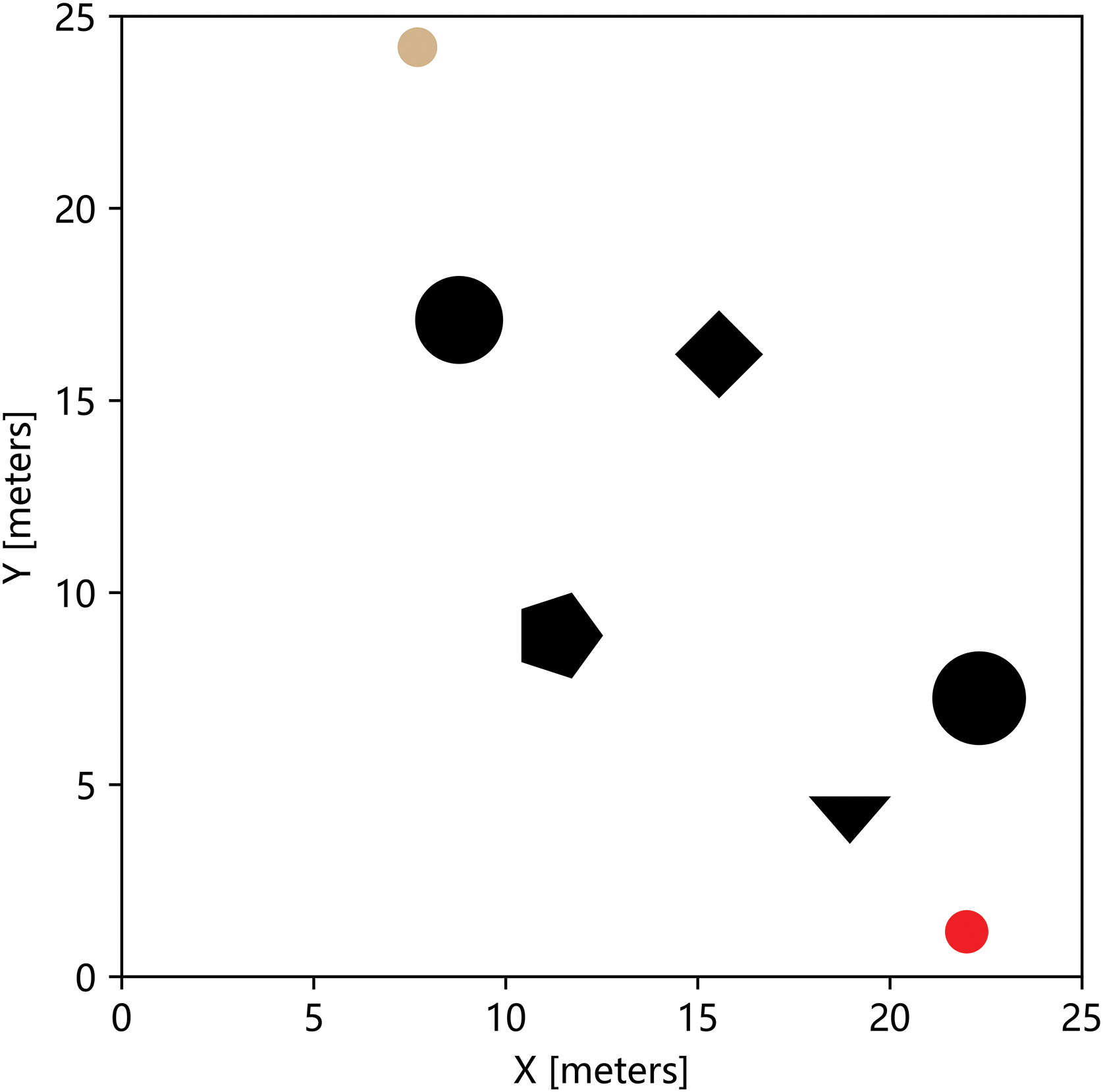
Figure 8: Example of random environment

In the random experimental scenario, by comparing the classical DDQN, MS-DDQN, ECMS-DDQN and AQRR-DDQN algorithm, it is evident that all four algorithms are able to plan a pathway to successfully arrive the target location without collision at the end of training. And Fig. 9 displays the reward curves of the four algorithms.

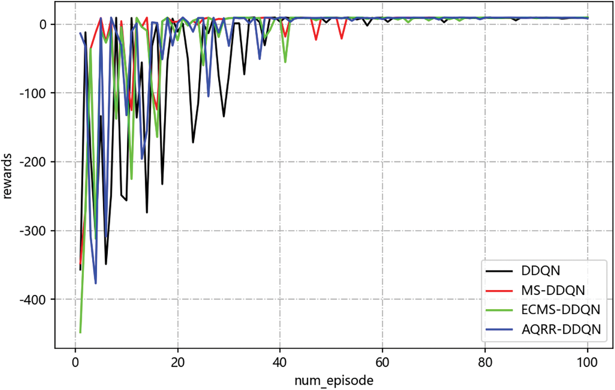
Figure 9: Return curves of four different algorithms for random environment

As seen in Fig. 9, throughout the entire training phase, every algorithm’s total return values have some fluctuations. But with the rise in the count of iteration episodes, the fluctuation becomes smaller and smaller and gradually converges. MS-DDQN algorithm fluctuates greatly in the middle period, and the remaining three algorithms are more stable obviously. And in the later stage, AQRR-DDQN is more stable than the other three algorithms, mainly because reward redistribution can better balance short-term and long-term returns and avoid over-reliance on short-term returns. This mechanism helps the model be more stable during exploration and reduces unnecessary reward fluctuations.

To verify the performance of the algorithms, test four algorithms in different random environments. Fig. 10 showed experimental results of the four algorithms in six random environments. The blue, orange, green and red curves are the path of DDQN algorithm, MS-DDQN algorithm, ECMS-DDQN algorithm and AQRR-DDQN algorithm separately.

Figure 10: Paths planned by four algorithms in six random environments

In Fig. 10, the trajectory planned by DDQN algorithm is the most tortuous, and in the environment with fewer obstacles, it is greatly affected by random disturbance, and obvious devolution phenomenon appears. The path steps planned by MS-DDQN, ECMS-DDQN, and the AQRR-DDQN algorithm are not obviously different. Every algorithm can successfully find the target location. In general, the AQRR-DDQN algorithm gives a smoother path.

Train the agent 100 times with different algorithms and compare the performance of different algorithms. Table 3 shows the results.

In Table 3, the AQRR-DDQN algorithm spent the shortest average time, while the DDQN algorithm spent the longest average time. The difference in time consumption between MS-DDQN and ECMS-DDQN is about 10 s. In terms of the average return, there is a small difference between DDQN and MS-DDQN, and the AQRR-DDQN algorithm has the highest average return. DDQN need the most average steps in path planning, and the difference between MS-DDQN and ECMS-DDQN is very small. The AQRR-DDQN algorithm is marginally ahead of the ECMS-DDQN by about 3 steps. From the point of view of the average reward per step, which can better reflect the algorithm’s performance, DDQN as a reference, the performance of MS-DDQN and ECMS-DDQN improved by about 3.50%, 5.59%, and the AQRR-DDQN improved by 8.33%, showing the best performance. The AQRR-DDQN algorithm achieves the expected results in different evaluation metrics. This is because adding discount round reward into the final reward of each action, which reduces the drawback of sparse reward. Meanwhile, sort the samples in the experience replay buffer according to reward value and prioritize the extraction of high-quality samples for learning reduces ineffective exploration and the exploration progress is speeded up.

5  Conclusions

Path planning is a key task in many autonomous intelligent systems, especially in complex and uncertain environments, effective path planning is crucial to the efficiency of task execution. The main route of this paper is to improve the path planning ability of the agent in a more efficient learning process by improving the DDQN algorithm. When using DDQN to realize path planning, agents often face two main challenges: slow convergence caused by sparse rewards, and insufficient use of high-quality experience limits the learning effect of agents. This paper solves the problem using the following methods: Average Q-value estimation is introduced into the DDQN algorithm to enhance the precision of the target Q-value. And a reward redistribution mechanism is proposed to redistribute the final reward of each action using trajectory information so that the agent can obtain feedback in time, which improves the learning efficiency. Furthermore, a reward-prioritized experience selection method is introduced to enhance the utilization efficiency of high-quality experience data to improve the algorithm’s performance.

To verify the effectiveness of this method, several experiments are carried out in the simulation environment. By comparing DDQN, MS-DDQN, ECMS-DDQN, and the AQRR-DDQN algorithm, the results indicated that the AQRR-DDQN algorithm is superior to the other three algorithms in the average time taken, the average return, the average number of steps, and the average reward per step, which improves the efficiency of path planning. However, although this paper conducts experiments in stochastic simulation environments, the complexity of these environments is still relatively simple compared to the real world. In practical applications, complex scenarios often contain more dynamic variables, such as moving obstacles and changing environmental characteristics, which are not fully simulated in current experiments. Future studies will consider testing it in more complex dynamic environments to improve its adaptability and generalization.

Acknowledgement: The authors wish to express sincere appreciation to the reviewers for their valuable.

Funding Statement: This research was funded by National Natural Science Foundation of China (No. 62063006); Guangxi Science and Technology Major Program (No. 2022AA05002); Key Laboratory of AI and Information Processing (Hechi University), Education Department of Guangxi Zhuang Autonomous Region (No. 2022GXZDSY003); Central Leading Local Science and Technology Development Fund Project of Wuzhou (No. 202201001).

Author Contributions: The authors confirm contribution to the paper as follows: study conception and design: Lieping Zhang, Jianchu Zou; data collection: Yameng Yin; analysis and interpretation of results: Lieping Zhang, Yilin Wang, Jianchu Zou; draft manuscript preparation: Jiansheng Peng, Xiaoxu Shi. All authors reviewed the results and approved the final version of the manuscript.

Availability of Data and Materials: The data that support the findings of this study are available from the corresponding author upon reasonable request.

Ethics Approval: Not applicable.

Conflicts of Interest: The authors declare that they have no conflicts of interest to report regarding the present study.

References

1. A. N. A. Rafai, N. Adzhar, and N. I. Jaini, “A review on path planning and obstacle avoidance algorithms for autonomous mobile robots,” J. Robot., vol. 2022, no. 1, Art. no. 2538220. doi: 10.1155/2022/2538220. [Google Scholar] [CrossRef]

2. L. Wang, X. Yang, Z. L. Chen, and B. R. Wang, “Application of the improved rapidly exploring random tree algorithm to an insect-like mobile robot in a narrow environment,” Biomimetics, vol. 8, no. 4, 2023, Art. no. 374. doi: 10.3390/biomimetics8040374. [Google Scholar] [PubMed] [CrossRef]

3. Y. N. Cui, J. Ren, and Y. Zhang, “Path planning algorithm for unmanned surface vehicle based on optimized ant colony algorithm,” IEEJ Trans. Electr. Electron. Eng., vol. 17, no. 7, pp. 1027–1037, 2022. doi: 10.1002/tee.23592. [Google Scholar] [CrossRef]

4. Y. X. Hou, H. B. Gao, Z. J. Wang, and C. S. Du, “Path planning for mobile robots based on improved A* algorithm,” presented at Int. Conf. Neur. Com. Adv. App., Jinan, China, Jul. 8–10, 2022. [Google Scholar]

5. S. Sundarraj, R. V. K. Reddy, M. B. Babu, G. H. Lokesh, F. Flammini and R. Natarajan, “Route planning for an autonomous robotic vehicle employing a weight-controlled particle swarm-optimized Dijkstra algorithm,” IEEE Access, vol. 11, pp. 92433–92442, 2023. doi: 10.1109/ACCESS.2023.3302698. [Google Scholar] [CrossRef]

6. T. X. Mao and H. Deng, “Path planning of slender tensegrities based on the artificial potential field method,” AIAA J., vol. 61, no. 5, pp. 2255–2265, 2023. doi: 10.2514/1.J062670. [Google Scholar] [CrossRef]

7. L. M. Ran, S. N. Ran, and C. M. Meng, “Green city logistics path planning and design based on genetic algorithm,” PeerJ. Comput. Sci., vol. 2023, no. 9, 2023, Art. no. e1347. doi: 10.7717/peerj-cs.1347. [Google Scholar] [PubMed] [CrossRef]

8. H. W. Qin, S. L. Shao, T. Wang, X. T. Yu, Y. Jiang and Z. H. Cao, “Review of autonomous path planning algorithms for mobile robots,” Drones, vol. 7, no. 3, 2023, Art. no. 211. doi: 10.3390/drones7030211. [Google Scholar] [CrossRef]

9. Y. Cao, K. Ni, T. Kawaguchi, and S. Hashimoto, “Path following for autonomous mobile robots with deep reinforcement learning,” Sensors, vol. 24, no. 2, 2024. doi: 10.3390/s24020561. [Google Scholar] [PubMed] [CrossRef]

10. S. G. Wen, Y. F. Jiang, B. Cui, K. Gao, and F. Wang, “A hierarchical path planning approach with Multi-SARSA based on topological map,” Sensors, vol. 22, no. 6, 2022, Art. no. 2367. doi: 10.3390/s22062367. [Google Scholar] [PubMed] [CrossRef]

11. Q. Zhou, Y. Lian, J. Y. Wu, M. Y. Zhu, H. Y. Wang and J. L. Cao, “An optimized Q-Learning algorithm for mobile robot local path planning,” Knowl. Based Syst., vol. 286, 2024, Art. no. 111400. doi: 10.1016/j.knosys.2024.111400. [Google Scholar] [CrossRef]

12. S. L. Du, Z. X. Zhu, X. F. Wang, H. G. Han, and J. F. Qiao, “Real-time local path planning strategy based on deep distributional reinforcement learning,” Neurocomputing, vol. 599, 2024, Art. no. 128085. doi: 10.1016/j.neucom.2024.128085. [Google Scholar] [CrossRef]

13. X. Y. Li et al., “Deep reinforcement learning for optimal rescue path planning in uncertain and complex urban pluvial flood scenarios,” Appl. Soft Comput., vol. 144, 2023, Art. no. 110543. doi: 10.1016/j.asoc.2023.110543. [Google Scholar] [CrossRef]

14. J. Escobar-Naranjo et al., “Autonomous navigation of robots: Optimization with DQN,” Appl. Sci., vol. 13, no. 12, 2023, Art. no. 7202. doi: 10.3390/app13127202. [Google Scholar] [CrossRef]

15. K. Demir, V. Tumen, S. Kosunalp, and T. Iliev, “A deep reinforcement learning algorithm for trajectory planning of swarm uav fulfilling wildfire reconnaissance,” Electronics, vol. 13, no. 13, 2024, Art. no. 2568. doi: 10.3390/electronics13132568. [Google Scholar] [CrossRef]

16. Y. Y. Huang, Z. W. Li, C. H. Yang, and Y. M. Huang, “Automatic path planning for spraying drones based on deep Q-Learning,” J. Internet Technol., vol. 24, no. 3, pp. 565–575, 2023. doi: 10.53106/160792642023052403001. [Google Scholar] [CrossRef]

17. E. Aljalbout, F. Frank, M. Karl, and P. van der Smagt, “On the role of the action space in robot manipulation learning and sim-to-real transfer,” IEEE Robot. Autom. Lett., vol. 9, no. 6, pp. 5895–5902, 2024. doi: 10.1109/LRA.2024.3398428. [Google Scholar] [CrossRef]

18. V. T. Ha and V. Q. Vinh, “Experimental research on avoidance obstacle control for mobile robots using Q-Learning (QL) and deep Q-Learning (DQL) algorithms in dynamic environments,” Actuators, vol. 13, no. 1, 2024, Art. no. 26. doi: 10.3390/act13010026. [Google Scholar] [CrossRef]

19. J. X. Li, Y. T. Chen, X. N. Zhao, and J. Y. Huang, “An improved DQN path planning algorithm,” J. Supercomput., vol. 78, no. 1, pp. 616–639, 2022. doi: 10.1007/s11227-021-03878-2. [Google Scholar] [CrossRef]

20. D. A. Deguale, L. L. Yu, M. L. Sinishaw, and K. Y. Li, “Enhancing stability and performance in mobile robot path planning with PMR-Dueling DQN algorithm,” Sensors, vol. 24, no. 5, 2024, Art. no. 1523. doi: 10.3390/s24051523. [Google Scholar] [PubMed] [CrossRef]

21. R. Q. Zhao, X. Lu, S. B. Lyu, J. H. Zhang, and F. S. Li, “Deep reinforcement learning based path planning for mobile robots using time-sensitive reward,” presented at 2022 19th ICCWAMTIP, Chengdu, China, Dec. 16–18, 2022. [Google Scholar]

22. F. H. Huang, Y. X. He, Y. Zhang, X. Y. Deng, and W. Jiang, “Controlling underestimation bias in reinforcement learning via minmax operation,” Chin. J. Aeronaut., vol. 37, no. 7, pp. 406–417, 2024. doi: 10.1016/j.cja.2024.03.008. [Google Scholar] [CrossRef]

23. X. H. Zhang, Z. Chen, Y. Zhang, Y. Liu, M. L. Jin and T. S. Qiu “deep-reinforcement-learning-based distributed dynamic spectrum access in multiuser multichannel cognitive radio internet of things networks,” IEEE Internet Things J., vol. 11, no. 10, pp. 17495–17509, 2024. doi: 10.1109/JIOT.2024.3359277. [Google Scholar] [CrossRef]

24. P. Wang, X. Q. Li, C. X. Song, and S. P. Zhai, “Research on dynamic path planning of wheeled robot based on deep reinforcement learning on the slope ground,” J. Robot., vol. 2020, no. 1, 2020, Art. no. 7167243. doi: 10.1155/2020/7167243. [Google Scholar] [CrossRef]

25. S. H. Jiang, S. J. Sun, and C. Li, “Path planning for outdoor mobile robots based on IDDQN,” IEEE Access, vol. 12, pp. 51012–51025, 2024. doi: 10.1109/ACCESS.2024.3354075. [Google Scholar] [CrossRef]

26. S. H. Yin and Z. R. Xiang, “Adaptive operator selection with dueling deep Q-network for evolutionary multi-objective optimization,” Neurocomputing, vol. 581, 2024, Art. no. 127491. doi: 10.1016/j.neucom.2024.127491. [Google Scholar] [CrossRef]

27. J. D. Zhao, Z. G. Gan, J. K. Liang, C. Wang, K. Q. Yue and W. J. Li, “Path planning research of a UAV base station searching for disaster victims’ location information based on deep reinforcement learning,” Entropy, vol. 24, no. 12, 2022, Art. no. 1767. doi: 10.3390/e24121767. [Google Scholar] [PubMed] [CrossRef]

28. X. H. Peng et al., “Enhanced autonomous navigation of robots by deep reinforcement learning algorithm with multistep method,” Sensors & Materials, vol. 33, no. 2, pp. 825–842, 2021. doi: 10.18494/SAM.2021.3050. [Google Scholar] [CrossRef]

29. X. Zhang, X. X. Shi, Z. Q. Zhang, Z. Z. Wang, and L. P. Zhang, “A DDQN path planning algorithm based on experience classification and multi steps for mobile robots,” Electronics, vol. 11, no. 14, 2022, Art. no. 2120. doi: 10.3390/electronics11142120. [Google Scholar] [CrossRef]

30. Z. Z. Chu, F. L. Wang, T. J. Lei, and C. M. Luo, “Path planning based on deep reinforcement learning for autonomous underwater vehicles under ocean current disturbance,” IEEE Trans. Intell. Vehicles, vol. 8, no. 1, pp. 108–120, 2023. doi: 10.1109/TIV.2022.3153352. [Google Scholar] [CrossRef]

31. X. F. Yang, Y. L. Shi, W. Liu, H. Ye, W. B. Zhong and Z. R. Xiang, “Global path planning algorithm based on double DQN for multi-tasks amphibious unmanned surface vehicle,” Ocean Eng., vol. 266, no. 5, 2022, Art. no. 112809. doi: 10.1016/j.oceaneng.2022.112809. [Google Scholar] [CrossRef]

32. O. Anschel, N. Baram, and N. Shimkin, “Averaged-DQN: Variance reduction and stabilization for deep reinforcement learning,” in Proc. 34th In Int. conf. Mach. Learn., 2017, pp. 176–185. [Google Scholar]

33. W. Yue, X. H. Guan, and L. Y. Wang, “A novel searching method using reinforcement learning scheme for multi-UAVs in unknown environments,” Appl. Sci., vol. 9, no. 22, 2019, Art. no. 4964. doi: 10.3390/app9224964. [Google Scholar] [CrossRef]

34. H. T. Meng and H. R. Zhang, “Mobile robot path planning method based on deep reinforcement learning algorithm,” J. Circuits, Syst. Comput., vol. 31, no. 15, 2022, Art. no. 2250258. doi: 10.1142/S0218126622502589. [Google Scholar] [CrossRef]

35. A. Devo, G. Costante, and P. Valigi, “Deep reinforcement learning for instruction following visual navigation in 3D maze-like environments,” IEEE Robot. Autom. Lett., vol. 5, no. 2, pp. 1175–1182, 2020. doi: 10.1109/LRA.2020.2965857. [Google Scholar] [CrossRef]