Enhancing Solar Energy Production Forecasting Using Advanced Machine Learning and Deep Learning Techniques: A Comprehensive Study on the Impact of Meteorological Data

1  Introduction

Solar photovoltaic (PV) systems are among the most popular renewable energy alternatives [1]. Many countries are transitioning to solar PV systems for large-scale electricity generation because they provide a clean, renewable energy source with minimal maintenance costs. However, photovoltaic energy production is highly dependent on uncontrollable weather and environmental factors such as module temperature, solar radiation, wind speed, wind pressure and direction, atmospheric temperature, and humidity. The power output of a photovoltaic system fluctuates dynamically over time due to the variability of these environmental factors. As a result, accurately forecasting photovoltaic energy production is quite challenging. The unpredictability of PV output significantly impacts the stability, reliability, and planning of power system operations, as well as economic benefits. Despite the numerous advantages of photovoltaic power generation systems over other renewable energy sources, there are still challenges to their large-scale integration. Variations in solar radiation, humidity, the presence of dust in the air, temperature, and wind speed can all significantly affect the variability of output power generated by photovoltaic systems. The uncertainty of these weather parameters complicates the accurate forecasting of expected output power from solar photovoltaic generation systems [2]. Consequently, this poses an obstacle to effective planning and pricing within the electricity system and networks.

Ukraine’s electricity system is a critical infrastructure, burdened with morally and technically outdated assets that still rely on carbon-intensive generation. Ukraine is facing serious energy security challenges due to missile attacks on energy facilities conducted by Russia. These attacks cause significant damage to the infrastructure, necessitating a rapid reorientation of the electrical grid towards a distributed generation system. One of the most urgent challenges is the rapid restoration of damaged infrastructure and its modernization to accommodate distributed generation.

The integration of large volumes of renewable energy sources, such as solar and wind power, requires the development and implementation of new network management algorithms. This includes predictive models for forecasting energy production, as well as management systems that can effectively respond to fluctuations in generation and energy consumption. The application of machine and deep learning methods in this context is becoming increasingly popular due to their ability to process large volumes of data and identify complex patterns.

Linear and Polynomial Regression: Linear regression is often used to forecast energy production based on historical data. Polynomial regression can be applied to account for nonlinear relationships between variables, such as solar radiation intensity and temperature. The biggest disadvantages of these methods are their ability to forecast only one point and their dependence on data drift, which is common for weather parameters [3]. The k-nearest neighbors method forecasts energy production by finding similar days in historical data and averaging their results. This method is simple to implement but may be inefficient with large datasets. Additionally, machine learning techniques, such as clustering, can be used to minimize the computational complexity of this method [4]. The support vector machine (SVM) method is used for forecasting by finding the optimal hyperplane that separates different classes of data. This method can be effective for short-term changes in energy production. SVM can also be used as part of an explainable module, offering insights into which features are most influential in the forecasting process [5]. Random Forest (RF), an ensemble method based on decision trees, provides more accurate predictions by combining the results of multiple trees. It is also robust to overfitting and performs well on various datasets. Additionally, RF can be part of feature extraction techniques [6].

Neural Networks: Neural networks are used for forecasting due to their ability to detect complex patterns in data. Specifically, Multilayer Perceptrons (MLP) and Recurrent Neural Networks (RNN) are popular for this task [7]. Recurrent Neural Networks (RNN) [8] and Long Short-Term Memory (LSTM) RNNs [9] are effective for processing time series data, as they consider dependencies between data points over time. LSTM is particularly useful for forecasting long-term trends. Convolutional Neural Networks (CNN) excel at identifying local patterns in data, such as seasonal trends, abrupt changes, and periodic behavior in energy production data. Although CNNs are typically used for image processing, they can also be applied to forecasting tasks where local patterns in data need to be considered. For example, in [10], CNNs are used to process meteorological maps and make predictions based on them.

Combining different machine and deep learning methods can improve forecasting accuracy. For example, combining CNN and LSTM allows for considering both local and temporal patterns in data [11]. Using ensemble models, such as gradient boosting or random forests, reduces forecasting error by combining the results of several base models [12–14].

Feature selection is a crucial step in the forecasting process, as it involves identifying the most relevant variables that influence solar energy production. Proper feature selection can enhance model performance, reduce computational complexity, and improve interpretability [15,16].

Forecasting solar panel energy production is a complex task requiring the use of advanced machine and deep learning methods. Literature sources indicate that applying various models. Each method has its advantages and disadvantages, and the choice of a specific model depends on the task’s characteristics and available data. This paper presents a comprehensive approach to predicting solar energy generation by leveraging detailed meteorological data and advanced machine learning techniques. The main contributions of this study include:

•   Data Collection and Preprocessing: A rich dataset was curated, spanning 14 months and comprising 10,464 rows with 27 features, detailing various weather conditions and solar energy metrics. Data was thoroughly preprocessed, including logarithmic transformations and the addition of sunrise and sunset information. This preprocessing helped in removing non-daylight hours, which corresponded to near-zero energy generation, thus refining the dataset to 6048 rows.

•   Model Development and Training: Multiple models were developed and trained, including SVM, KNN, H2O AutoML, CatBoost, LSTM, and LSTM with Inception layers, each tailored to handle the specificities of the dataset. Specific adaptations were made for each model type, such as one-hot encoding for LSTM models and specifying categorical features for CatBoost.

•   Rule-Based Prediction Wrapper: A novel rule-based (hour-based) prediction wrapper was introduced to enhance model performance by restricting predictions to daylight hours. This wrapper utilized external sunrise and sunset data, ensuring that predictions were only made during hours with potential solar energy generation.

•   Stacking Model Enhancement: The cascaded stacking model for enhancing solar energy production forecasting was proposed, incorporating association rules, weak predictors, and a modified stacking aggregation procedure to enhance generalization and reduce prediction errors.

The rest of the paper is organized as follows: Section 2 presents the main models utilized in the paper; Section 3 explains the obtained results of the proposed model; Section 4 compares the results; and finally, the last section concludes the paper.

2  Materials and Methods

2.1 Data Exploratory Analysis

The dataset appears to contain weather and solar energy production data. Meteorological data for the analysis were obtained from https://www.visualcrossing.com/ (accessed on 02 July 2024), which provides historical and forecasted weather data. The location of the solar power station studied is Radekhiv, Lviv region, Ukraine. An important aspect is that the nearest weather stations are located at distances of 64 and 72 km from the solar station, which can cause significant errors in the meteorological data. This affects the accuracy of energy production forecasting, as even minimal errors in input data can lead to substantial deviations in the forecasts [17]. The hourly generated solar energy data are obtained from a commercial accounting metering point. A dataset spanning 14 months of solar generation activity was gathered to train and evaluate the prediction models. The raw dataset contains 10,464 rows of data and 14 columns that describe generation, solar radiation, solar energy, UV index, temperature (Celsius), humidity level, cloud cover, visibility (kilometers), and the elevation and azimuth angles of a solar panel at a certain hour, day, month, and year.

Initially, instance selection was performed, resulting in the removal of 0.2% of missing data. Subsequently, an analysis of the initial features was conducted. The dataset contains comprehensive meteorological data, which can be utilized for forecasting solar energy production. The distribution of various features in relation to the target variable, “generation,” is presented in Fig. 1.

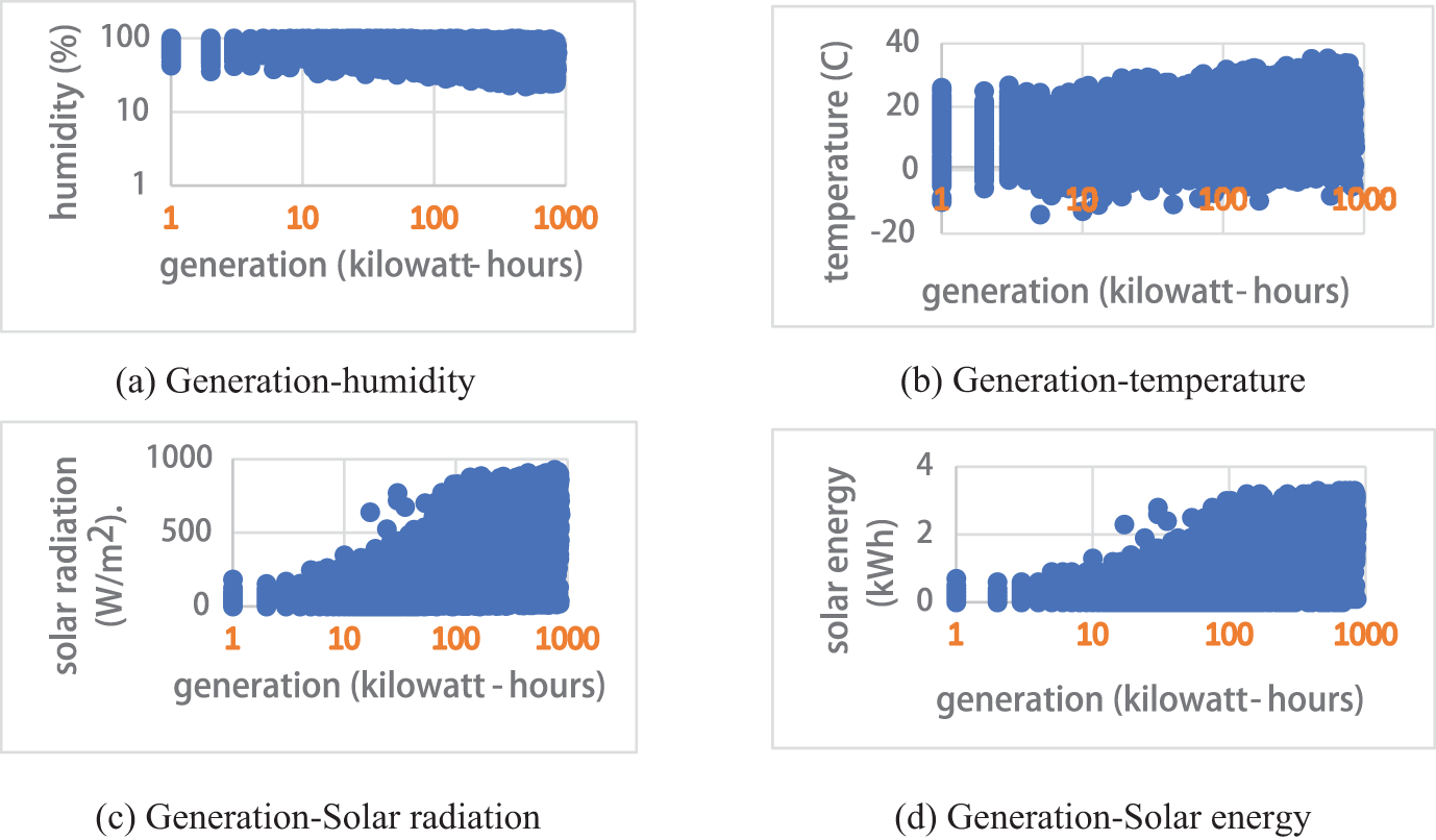
Figure 1: Initial data distribution

Generally, there is an inverse relationship between humidity and solar energy generation (Fig. 1a). Higher humidity means more water vapor in the air, which can scatter and absorb solar radiation, reducing the amount of sunlight that reaches the solar panels. Therefore, as humidity increases, solar energy generation typically decreases. Temperature affects solar panel efficiency. Generally, solar panels are less efficient at higher temperatures (Fig. 1b). There is often an optimal temperature range where solar panels operate most efficiently. Outside this range, especially at higher temperatures, efficiency drops. The graph shows a peak where the temperature is optimal for maximum generation (parabolic trend), with generation decreasing at temperatures above and below this peak. Solar radiation directly impacts the amount of energy generated by solar panels. More solar radiation generally results in higher energy production (Fig. 1c). This relationship is typically positive and linear. The graph shows an upward trend, indicating that increased solar radiation leads to higher solar energy generation. Fig. 1d shows the relationship between the total solar energy received (input) and the solar energy generated (output). This is a direct correlation between the solar energy received and the energy generated, but inefficiencies and losses in the system can affect this relationship. The graph shows a linear trend with a slope of less than 1, indicating that not all received solar energy is converted into electrical energy due to inefficiencies.

To better understand the nature of data, a self-organizing map (SOM) is used (Fig. 2). SOM uses a neighborhood function to preserve the topological properties of the input space [18,19]. The majority of the hexagons are blue (Fig. 2), indicating that most of the data points fall within the 0–200 range. There are a few hexagons with other colors, such as green, yellow-green, and yellow, indicating higher densities in those regions. The areas with light yellow hexagons represent the highest density of data points (≥800). Finally, a white box indicates that the correlation is not significantly different from 0 at the specified significance level (in this example, at α = 5%) for a couple of variables. A correlation not significantly different from 0 means that there is no linear relationship between the two variables considered in the population (there could be another kind of association, but not linear).

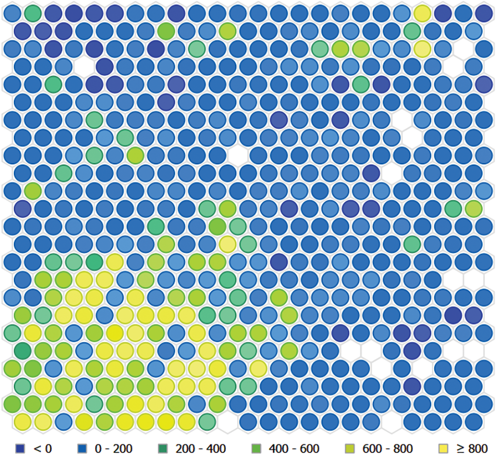
Figure 2: SOM result

To determine whether a specific correlation coefficient is significantly different from 0, a correlation test has been performed based on two factors: the number of observations and the correlation coefficient. The more observations and the stronger the correlation between 2 variables, the more likely it is to reject the null hypothesis of no correlation between these 2 variables. The ranked cross-correlated features are given in Fig. 3. The significance level for the correlation test used as less than 0.05.

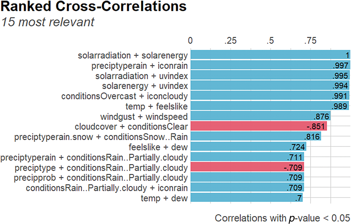
Figure 3: 15 Most correlated features

Based on this result, one feature from each pair must be removed. To do that, feature selection methods are used.

2.2 Data Preparation

Feature selection remains a vital step in the development of accurate and efficient solar energy production forecasting models. Traditional methods like filter, wrapper, and embedded techniques continue to be widely used, while advanced and hybrid approaches offer promising improvements in handling complex and high-dimensional data [20,21].

Firstly, embedded methods for feature extractions are used. These methods perform feature selection during the model training process. Random Forest and Decision tree were implemented. The results are as follows:

•   Random forest: hour, solarradiation, humidity, solarenergy, feelslike, month;

•   Decision tree: solarradiation, hour.

Both methods show that “solarradiation” and “hour” are the most important features for generation prediction. On another side, “solarenergy” can be excluded as a highly correlated feature.

Secondly, an extension of the Random Forest algorithm, Boruta [22] algorithm was implemented. Boruta performs a more comprehensive search for relevant features by comparing the importance of original features to that of randomized shadow features. Column “solarradiation” has the highest importance score, indicating it is the most significant variable in the model. Columns “solarenergy” and “temp” also have high importance scores, making them key contributors to the model’s predictions. Features “shadowMin” and “shadowMax” have the lowest importance scores, suggesting they contribute the least to the model. Variables like “feelslike,” “month,” “uvindex,” “windgust,” and “winddir” fall in the middle range of importance scores. As a result, for the classical machine learning algorithm, “solarradiation”, “feelslike”, “hour”, “humidity” and “month” features were selected.

Next, data normalization is used. All the features, except hour, day, month, and year, have been logarithmically transformed (log1p). Additionally, the dataset was enriched with the sunrise and sunset hours scraped for every row from external sources (https://dateandtime.info/) (accessed on 02 July 2024). The resulting sunrise and sunset columns are linked to the month, day, hour, and year columns. This additional information was used to remove all the rows where the hour column does not fall into the daylight hours range of a specified day. This resulted in the removal of about 45% of all the rows which correspond to near- or zero energy generation. Finally, the year column is removed from the dataset. The final size of the stripped dataset is 6048 rows.

The dataset was split into training and evaluation parts utilizing time split with ratios of 80/20, respectively.

2.3 Utilized Models

Three alternative versions of the raw and stripped datasets were created:

•   A dataset for training the ML-based models and ensemble;

•   A dataset for training the LSTM-based models;

•   A dataset for training the CatBoost and H2O AutoML models.

When it comes to the former versions, every value that corresponds to hour, day, and month columns has been column-wise one-hot encoded [23]. Moreover, the data was transformed into sliding windows of size 8 h and stride 1. The grid search was implemented for hyperparameter tuning. The latter versions, however, do not have such transformations applied since libraries that are used to train CatBoost [24] and H2O AutoML [25] come with specific functionalities implemented to specify the categorical columns before or during the training.

ML-based models and ensembles benefit from one-hot encoding and sliding windows to capture temporal dependencies and handle categorical data. LSTM models excel at time series predictions, utilizing the sequential structure of the data without needing extensive preprocessing like one-hot encoding. CatBoost and H2O AutoML offer the flexibility to handle categorical features without preprocessing, streamlining the workflow while delivering high performance through automated and gradient-boosting techniques. In comparison to other similar models, these techniques were selected because they are known for their robustness, scalability, and ease of use in practical applications. The LSTM with Inception layers was selected for its ability to capture long-term dependencies in time-series data, which is crucial in solar energy generation tasks. Each of these models and data preprocessing steps was chosen to leverage the specific strengths of different machine learning techniques in handling time-dependent, categorical, and numerical data for solar energy forecasting. A few different models were utilized to predict the power generated by the solar panel:

•   ML-models such as:

•   linear regression (lm), k-nearest neighbors (knn),

•   SVM with linear kernel (ksvm),

•   SVM with polynomial kernel (svm polynomial),

•   SVM with the radial-basic kernel (svm rb),

•   FNN with one hidden layer and 4 neurons in this layer, 200 epochs, with weight decay of 0.01 to prevent overfitting (NN),

•   regression tree (CART algorithm, 5 trees, max depth 5) (regression tree);

•   Novel ensemble model;

•   H2O AutoML;

•   CatBoost;

•   LSTM;

•   LSTM with Inception blocks.

The novel cascaded stacking model. The baseline of the proposed cascaded stacking model for enhancing solar energy production forecasting consists of the following steps:

1.    In the first layer, association rules are built for hidden dependencies mining. Apriori algorithm was implemented. The whole dataset is used.

2.    In the second layer, weak predictors are chosen for the dataset consisting of important features.

3.    A modified stacking aggregation procedure is implemented.

The main disadvantage of the existing stacking models is that the meta-attributes on training and the test are different [26]. The meta-attribute in the training sample is not the answers of a particular regressor; it consists of pieces that are the answers of various regressions (with different coefficients). The meta-attribute on the control sample, in general, is the answer to a completely different regression, tuned to the full training. In classic stacking, the situations can arise when a meta-attribute contains few unique values, but many of these values do not intersect in training and testing. The developed stacking model also combines several weak predictors. In addition, the meta-features are deformed based on the results of pairwise multiplication. The meta-features are the results of weak predictors training. In the end, contorted features are used together with the training dataset in the meta-model. This combination avoids the correlation of weak predictors results and increases the model generalization. On the other hand, the correlation matrix shows a lot of weak dependencies in the dataset, which can be found using association rules. It means the possibility of discovering interesting relations between variables in the database. It allows the creation of new features based on the presence of certain itemsets and patterns found in the rules. These features are added to the original dataset.

The general proposed schema is given in Fig. 4. As a metamodel, random forest is used. Grid Search was used for parameters choosing. Parameters of RF are the following: max dept = 3, max number of trees = 100, Mean Squared Error as criteria, the minimum number of samples required to split an internal node is equal to 3, bootstrap usage.

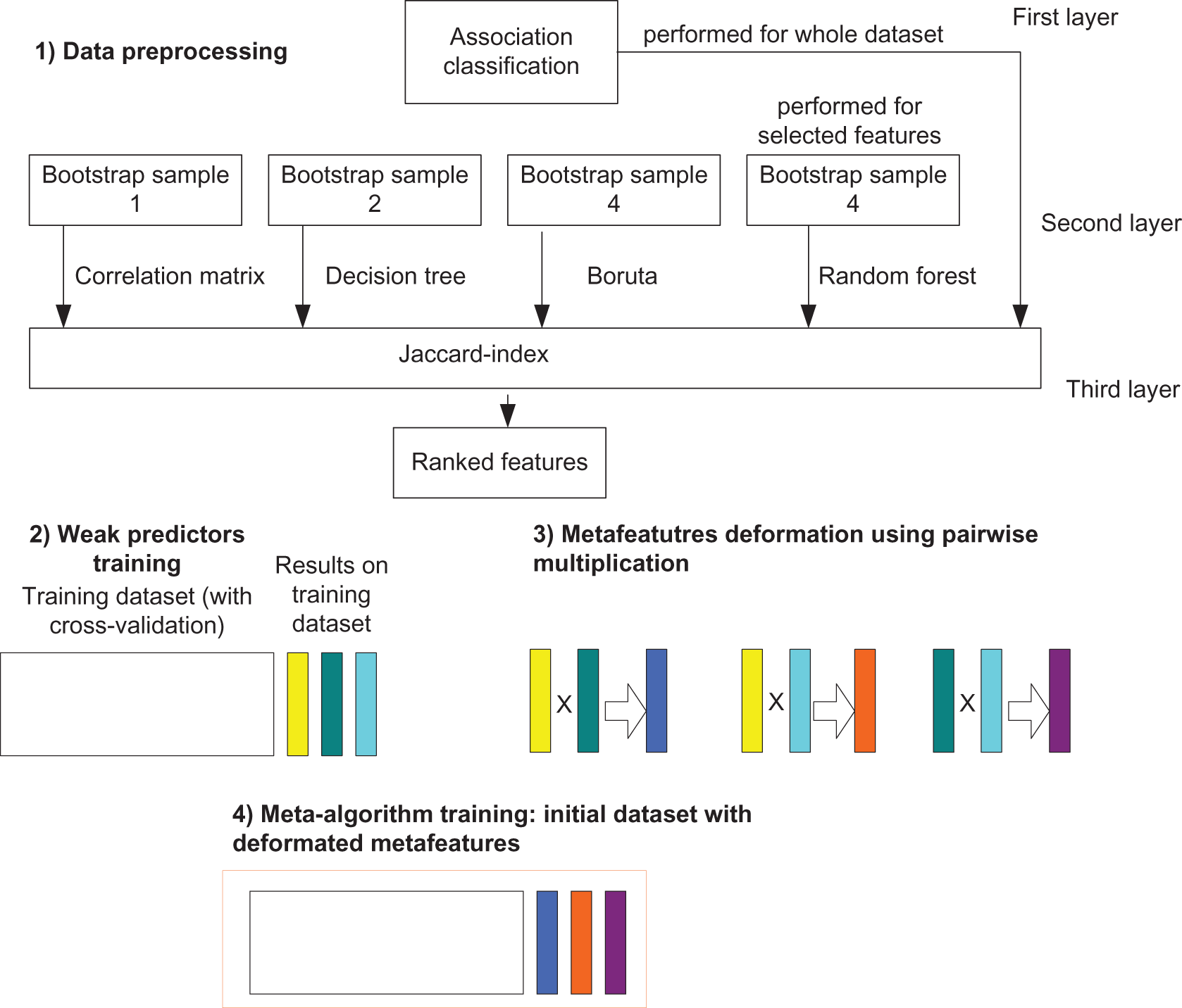
Figure 4: Proposed cascaded stacking model for enhancing solar energy production forecasting

H2O AutoML. H2O AutoML is an automated machine-learning platform that aims to simplify the process of building machine-learning models. It is part of the H2O.ai ecosystem, which provides tools and libraries for scalable and distributed machine learning. H2O AutoML explores a variety of machine-learning models and techniques to find the best-performing model for a given dataset. Some of the models it may try include gradient boosting machines (GBM), random forest ensembles, deep neural networks, generalized linear models (GLM), XGBoost, and LightGBM. In this work, H2O AutoML was initialized with the max_models parameter set to 30 to reduce the training time. Both training and evaluation splits of the dataset were transformed into H2OFrame objects, and the factor method was called on categorical columns such as hour, day, and month.

CatBoost. CatBoost is a powerful gradient-boosting library that is specifically designed for categorical feature handling and efficient training. It employs gradient boosting, which is an ensemble learning technique that builds a series of decision trees iteratively, each tree correcting errors made by the previous ones. This leads to improved predictive accuracy and robustness. CatBoost can handle categorical variables directly, using techniques like target encoding and one-hot encoding internally. This simplifies the preprocessing steps and often leads to better model performance. CatBoost was initialized with the iterations parameter set to 2000 and task_type set to ‘GPU’ to utilize the graphics card available for training and inference. The fit method was supplied with a cat_features parameter specifying the categorical features of the dataset.

LSTM. LSTM was initialized with TensorFlow and Keras libraries. The model is defined as a Sequential model, which means layers are added sequentially [27]. The architecture is as follows:

•   The first layer added is an LSTM layer with 24 units, using the ReLU activation function and set to return sequences (return_sequences = True). X_train determines the input shape.shape [1] (number of time steps or features) and X_train.shape [2] (number of features per time step).

•   The second layer is another LSTM layer with 48 units, also using the ReLU activation function and set to return sequences.

•   The third layer is an LSTM layer with 96 units, again using the ReLU activation function but this time set not to return sequences (return_sequences = False).

•   Finally, a Dense layer with 1 unit is added, representing the regression task output layer.

Adam optimizer is used for training with an initial learning rate set to 0.001; the loss function is a mean squared error, while tracked metrics also include mean absolute error. The number of train epochs and batch size were set to 100 and 128, respectively. Early stopping is used with val_loss monitored metric, patience set to 10.

LSTM with Inception Layers. LSTM with Inception layers’ architecture combines convolutional layers with an LSTM layer, incorporating an inception module for feature extraction [28]. Description of the utilized steps:

1.    The input data goes through a series of convolutional layers (Conv2D) with different kernel sizes and strides, followed by LeakyReLU activation functions. This block extracts features from the input data. After the convolutional block, an inception module is constructed. It includes three branches: convolutional layers with kernel size (3, 1) for capturing local patterns, convolutional layers with kernel size (5, 1) for capturing larger patterns, and max pooling followed by a convolutional layer for downsampling and feature extraction.

2.    The outputs from these branches are concatenated along the channel axis. The concatenated output from the inception module is reshaped and then passed through a dropout layer with a dropout rate of 0.2. Dropout helps in regularizing the model by randomly setting a fraction of input units to zero during training. The reshaped and dropout-transformed data is fed into an LSTM layer with 64 units.

3.    Finally, the output from the LSTM layer is passed through a Dense layer with 1 unit (for regression tasks).

The model is compiled with the Adam optimizer, mean squared error loss, and mean absolute error metric. The number of epochs and batch size are 200 and 128, respectively. During training, model checkpoints are saved based on the validation loss to track the best-performing model.

Hour-Based Prediction Wrapper. An additional rule-based (hour-based) prediction wrapper was introduced to maximize the performance of prediction models. It is specifically tailored to utilize the trained models only during daylight hours of a given day [29]. This functionality is enabled given the sunset and sunrise data. It is supplied as a separate data frame with sunset and sunrise hours of specified days and months, covering a year, preferably one with 29-day February for completeness. Internally, implemented in this study class checks if the input hour corresponds to daylight hours using the provided daylight data frame. Predictions are made using the trained model, and non-daylight hour predictions are set to zero before returning the final predicted values. The use of this wrapper is aimed at maximizing the performance of trained models by ensuring their applicability only during daylight periods, contributing to more accurate solar energy predictions.

3  Results

Metrics such as Mean Squared Error (MSE), Coefficient of determination (R2), and Mean Absolute Error (MAE) are used for ML-models while MSE and MAE are implemented for the rest of models. CatBoost and H2O AutoML models are gradient-boosting techniques and automated machine learning systems, respectively, that excel at handling large datasets with complex relationships. These models are optimized for minimizing prediction error, and therefore metrics like MSE and MAE are often prioritized because they give a direct indication of how close the predictions are to the actual values. R2, while informative in some cases, can be less interpretable for gradient-boosting models, especially when dealing with datasets that have complex interactions between features, as in solar energy forecasting. These models may produce highly accurate predictions, but the variance captured by R2 may not fully reflect the performance of the model in terms of minimizing error. MSE and MAE provide more tangible insights into how well the model is performing by focusing on error magnitude, making them more appropriate metrics for this task.

Table 1 presents the results of ML models implementation. K-Nearest Neighbors (knn) performs best among the models, with very low MSE, high R2, and low MAE. Regression Tree is also a strong performer, while Neural Networks (NN) and Linear Model (lm) have the worst performance.

Table 2 presents the result of ensemble implementation. One additional feature was created based on association rules mining.

The Ensemble model outperforms all the previous models (including knn) in terms of MSE, R2, and MAE. It provides the best fit to the data with minimal prediction errors and explains the variance in the data almost perfectly. This suggests that the Ensemble model is highly effective for this particular dataset. Minimizing absolute error (AE) is crucial in generation prediction, as it directly impacts the accuracy and reliability of forecasts. AE at the test dataset for several ML models is presented below (Fig. 5).

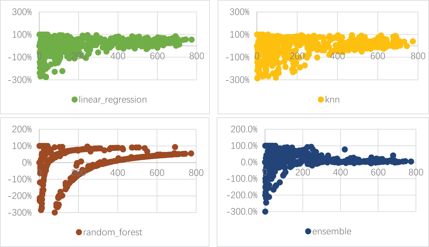
Figure 5: Error distribution for several models

The significant spread and presence of large errors suggest that the linear regression model may not be capturing the underlying patterns in the data well. High errors, especially negative ones, indicate that the model might be underfitting. The scatter plot for the KNN model shows a much more concentrated error distribution around the 0% line, indicating better accuracy and reliability than the linear regression model. The scatter plot for the Random Forest model indicates a high degree of accuracy, with errors becoming more concentrated and smaller as predicted values increase. This pattern suggests that the Random Forest model is particularly effective for higher predicted values and generally maintains a lower error rate than linear regression and KNN models. The overall error distribution highlights Random Forest’s robustness and reliability in generation forecasting. Compared to the Linear Model and KNN, the Random Forest model likely has lower AE and more tightly clustered errors, suggesting better overall performance. The error distribution for a novel ensemble is small for large numbers (300 and higher) and sufficient for small numbers. This model shows the best results but still has huge errors especially for small value of generation.

Although KNN demonstrated strong performance (R2 = 0.997), the authors introduced advanced ML and DL models to improve prediction accuracy, especially in handling complex patterns in data. KNN, while effective, may struggle with large datasets and does not generalize as well when compared to more sophisticated models like Random Forest or ensemble methods. More advanced techniques such as LSTM and ensemble models are used to capture nonlinear dependencies and temporal patterns, which are critical for solar energy forecasting. DL models are developed and tested. All the DL models were trained and scored on both raw and stripped versions of dataset, contributing to 8 models trained. All the trained models were additionally wrapped into hour-based prediction wrappers described above to maximize their prediction performance. Trained model names are composed as <model type>_<train dataset type> (Table 3).

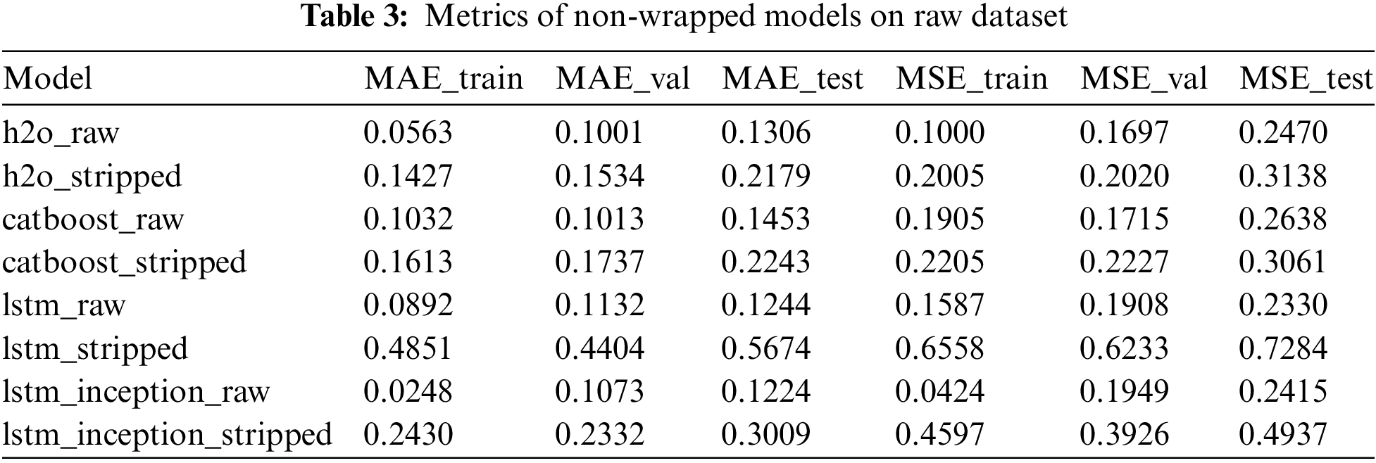
The h2o_raw model demonstrates efficient performance with low errors across all sets. Its MSE values are also low, indicating minimal prediction errors. The h2o_stripped model, on the other hand, shows higher errors compared to h2o_raw. This indicates a decrease in efficiency due to the reduced feature set. The catboost_raw model is also efficient. The catboost_stripped model shows higher errors compared to catboost_raw. This follows the trend observed in the h2o models, where the stripped feature set reduces efficiency. The lstm_raw model is highly efficient. Its MSE values are low and stable, indicating a strong performance comparable to h2o_raw. The lstm_stripped model shows significantly higher errors. The lstm_inception_raw model exhibits very low errors in training. The lstm_inception_stripped model shows higher errors compared to lstm_inception_raw. The most efficient models are lstm_inception_raw, h2o_raw, and lstm_raw, with consistently low errors.

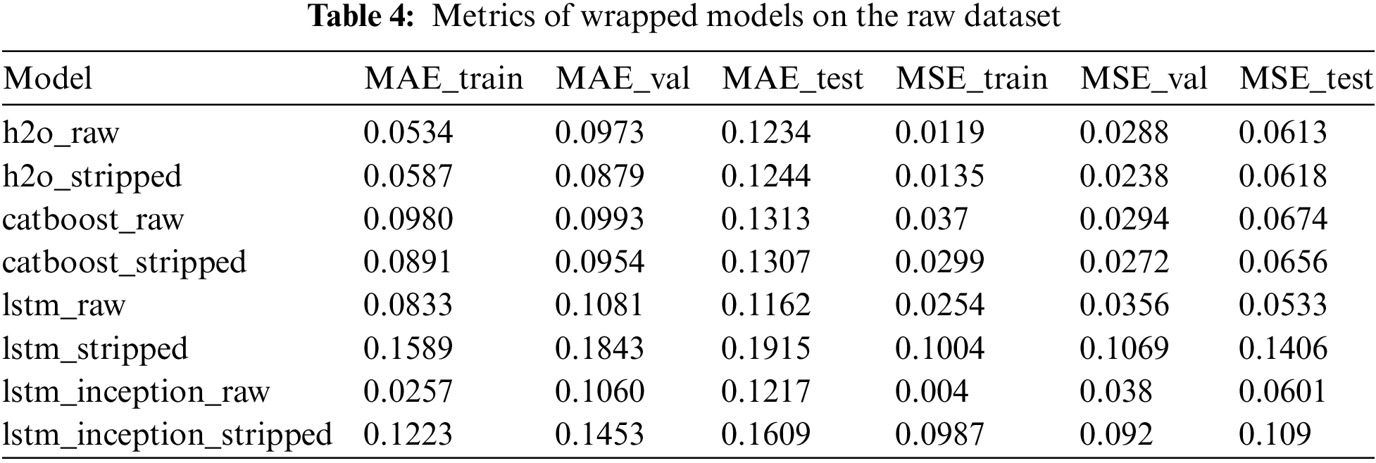
Table 4 presents the metrics of wrapped models on the raw dataset. Some models, such as the LSTM with Inception layers and H2O-based models, achieved low MAE values. The ensemble model with an MAE of 4.13208 and R2 = 0.999 indicates very high accuracy, and models with even lower MAEs (between 0.1 and 0.2) would likely reach similarly high R2 values, close to 1. However, R2 might not change significantly with small decreases in MAE since it is more sensitive to the explained variance, and not just prediction error. The most efficient models are lstm_inception_raw, h2o_raw, and lstm_raw, with consistently low errors across all sets.

Figs. 6 and 7 demonstrate the metrics of non-wrapped and wrapped models, respectively. Wrapped models generally show improved performance, with reduced prediction errors. Models like lstm_inception_raw demonstrate even better accuracy. The lstm_raw model exhibits the widest range of errors, indicating higher variability and possibly lower stability. Models trained on the stripped dataset tend to have slightly different error distributions compared to those trained on the raw dataset, but the pattern of stability in certain models (like h2o_stripped and catboost_stripped) remains. Models like h2o_stripped and catboost_stripped show lower and more stable error distributions.

Figure 6: Metrics of non-wrapped models on raw dataset

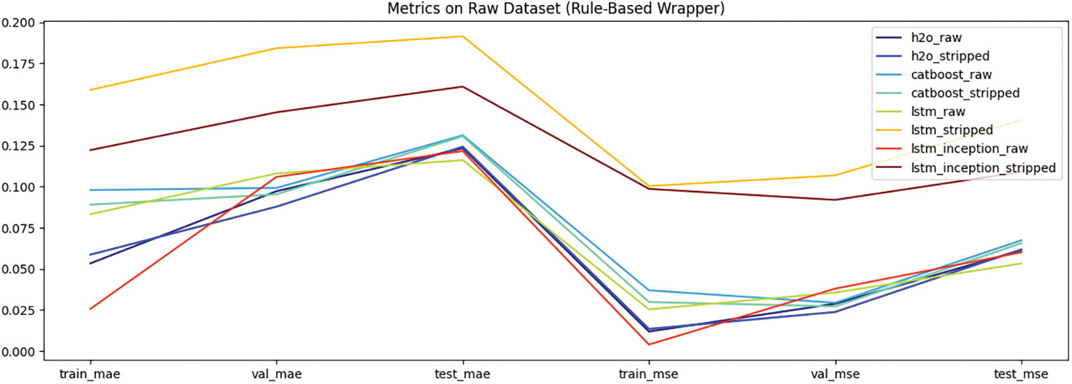
Figure 7: Metrics of wrapped models on raw dataset

Figs. 8 and 9 represent model scores on stripped data, emphasizing the error metrics. The h2o_stripped and catboost_stripped models consistently show lower and more stable error distributions across all datasets and stages. The lstm_raw model exhibits the widest range of errors, indicating higher variability and possibly lower stability. Models trained on the stripped dataset tend to have slightly different error distributions compared to those trained on the raw dataset, but the pattern of stability in certain models (like h2o_stripped and catboost_stripped) remains.

Figure 8: Scores of non-wrapped models on stripped dataset

Figure 9: Scores of wrapped models on stripped dataset

4  Discussion

The discussion of the results is framed around the broader context of Sustainable Development Goals (SDGs). In particular, this study directly contributes to SDG 7: Affordable and Clean Energy, SDG 9: Industry, Innovation, and Infrastructure, and SDG 13: Climate Action. The ensemble models, especially on raw data, provide a more accurate and robust approach for predicting solar energy generation, as demonstrated by their lower MSE, R2, and MAE values. These improvements in prediction accuracy have direct implications for enhancing the efficiency of renewable energy integration into power grids, which is crucial for SDG 7. By optimizing solar energy forecasting, the study supports more reliable and sustainable energy management, reducing the need for fossil fuel backup and improving the overall stability of renewable energy systems.

The LSTM with Inception layers performed best across all datasets, particularly when trained on raw data. This aligns with the goals of SDG 9, as adopting advanced machine learning models can lead to smarter and more resilient energy infrastructure. Applying a rule-based wrapper further enhanced model performance by optimizing predictions during daylight hours. This result underscores the potential for practical applications in real-time energy management systems, supporting SDG 13 by enabling more responsive and efficient use of solar energy resources. By improving the ability to predict energy output based on temporal patterns, the models contribute to reducing carbon emissions by promoting the use of clean energy sources. In comparing the performance of models on raw vs. stripped data, it is clear that maintaining rich, unprocessed datasets leads to better outcomes. This further emphasizes the importance of harnessing comprehensive datasets to support SDG 9. The ability to capture hidden dependencies in the data, particularly through the cascaded stacking model, supports better decision-making processes in implementing renewable energy systems.

5  Conclusion

A comprehensive dataset spanning 14 months of solar generation activity was analyzed, containing detailed meteorological data critical for forecasting solar energy production. This study demonstrates the potential of combining detailed meteorological data with advanced machine learning techniques to accurately predict solar energy generation. The integration of feature importance analysis, robust preprocessing, and innovative model architectures, along with rule-based enhancements, significantly improves prediction accuracy, making this approach highly valuable for efficient solar energy management and planning. Models trained on raw data generally performed better than those trained on stripped data. The hour-based prediction wrapper improved performance, especially for models trained on raw data. LSTM with Inception layers model, particularly on raw data, proved to be the most effective for predicting solar energy generation, with significant performance improvements achieved through feature selection, data preprocessing, and innovative modeling techniques. The novel cascaded stacking model for enhancing solar energy production forecasting shows good results too for the prediction of one-point data.

To further enhance the prediction accuracy and reliability of solar energy production forecasts, the following steps are planned:

•   To explore additional meteorological features and their interactions to improve model input.

•   To incorporate real-time meteorological data for dynamic and adaptive forecasting models.

Acknowledgement: The authors would like to thank the Armed Forces of Ukraine for providing security to perform this work.

Funding Statement: This research was funded by the H2020 Project ZEBAI.

Author Contributions: The authors confirm their contribution to the paper as follows: study conception and design: Nataliya Shakhovska, Mykola Medykovskyi, Oleksandr Gurbych; data collection: Mykhailo Melnyk; analysis and interpretation of results: Mykhailo Mamchur, Mykhailo Melnyk; draft manuscript preparation: Nataliya Shakhovska, Mykhailo Mamchur. All authors reviewed the results and approved the final version of the manuscript.

Availability of Data and Materials: The data that support the findings of this study are openly available in Figshare at https://figshare.com/articles/dataset/Solar_power_station_data/26357059/1?file=47875348 (accessed on 02 July 2024).

Ethics Approval: Not applicable.

Conflicts of Interest: The authors declare that they have no conflicts of interest to report regarding the present study.

References

1. K. N. Nwaigwe, P. Mutabilwa, and E. Dintwa, “An overview of solar power (PV systems) integration into electricity grids,” Mater. Sci. Energy Technol., vol. 2, no. 3, pp. 629–633, 2019. doi: 10.1016/j.mset.2019.07.002. [Google Scholar] [CrossRef]

2. R. Ahmed, V. Sreeram, Y. Mishra, and M. D. Arif, “A review and evaluation of the state-of-the-art in PV solar power forecasting: Techniques and optimization,” Renew. Sustain. Energ. Rev., vol. 124, no. 4, 2020, Art. no. 109792. doi: 10.1016/j.rser.2020.109792. [Google Scholar] [CrossRef]

3. M. AlShafeey and C. Csáki, “Evaluating neural network and linear regression photovoltaic power forecasting models based on different input methods,” Energy Rep., vol. 7, pp. 7601–7614, 2021. doi: 10.1016/j.egyr.2021.10.125. [Google Scholar] [CrossRef]

4. Y. Dong, X. Ma, and T. Fu, “Electrical load forecasting: A deep learning approach based on K-nearest neighbors,” Appl. Soft Comput., vol. 99, 2021, Art. no. 106900. doi: 10.1016/j.asoc.2020.106900. [Google Scholar] [CrossRef]

5. J. Shi, W. J. Lee, Y. Liu, Y. Yang, and P. Wang, “Forecasting power output of photovoltaic systems based on weather classification and support vector machines,” IEEE Trans. Ind. Appl., vol. 48, no. 3, pp. 1064–1069, 2012. doi: 10.1109/TIA.2012.2190816. [Google Scholar] [CrossRef]

6. J. Huertas Tato and M. Centeno Brito, “Using smart persistence and random forests to predict photovoltaic energy production,” Energies, vol. 12, no. 1, 2018, Art. no. 100. doi: 10.3390/en12010100. [Google Scholar] [CrossRef]

7. C. D. Dumitru, A. Gligor, and C. Enachescu, “Solar photovoltaic energy production forecast using neural networks,” Procedia Technol., vol. 22, no. 4, pp. 808–815, 2016. doi: 10.1016/j.protcy.2016.01.053. [Google Scholar] [CrossRef]

8. N. Shabbir, L. Kutt, M. Jawad, M. N. Iqbal, and P. S. Ghahfaroki, “Forecasting of energy consumption and production using recurrent neural networks,” Adv. Electr. Electron. Eng., vol. 18, no. 3, pp. 190–197, 2020. doi: 10.15598/aeee.v18i3.3597. [Google Scholar] [CrossRef]

9. F. Harrou, F. Kadri, and Y. Sun, “Forecasting of photovoltaic solar power production using LSTM approach,” in Advanced Statistical Modeling, Forecasting, and Fault Detection in Renewable Energy Systems, London, UK, 2020. [Google Scholar]

10. A. Agga, A. Abbou, M. Labbadi, and Y. El Houm, “Convolutional neural network (CNN) extended architectures for photovoltaic power production forecasting,” in 2021 9th Int. Conf. Smart Grid Clean Energy Technol. (ICSGCE), IEEE, 2021, pp. 104–108. [Google Scholar]

11. E. M. Al-Ali et al., “Solar energy production forecasting based on a hybrid CNN-LSTM-transformer model,” Mathematics, vol. 11, no. 3, 2023, Art. no. 676. doi: 10.3390/math11030676. [Google Scholar] [CrossRef]

12. K. Bogner, F. Pappenberger, and M. Zappa, “Machine learning techniques for predicting the energy consumption/production and its uncertainties driven by meteorological observations and forecasts,” Sustainability, vol. 11, no. 12, 2019, Art. no. 3328. doi: 10.3390/su11123328. [Google Scholar] [CrossRef]

13. P. P. Phyo, Y. C. Byun, and N. Park, “Short-term energy forecasting using machine-learning-based ensemble voting regression,” Symmetry, vol. 14, no. 1, 2022, Art. no. 160. doi: 10.3390/sym14010160. [Google Scholar] [CrossRef]

14. M. AlKandari and I. Ahmad, “Solar power generation forecasting using ensemble approach based on deep learning and statistical methods,” Appl. Comput. Inform., vol. 20, no. 3/4, pp. 231–250, 2024. doi: 10.1016/j.aci.2019.11.002. [Google Scholar] [CrossRef]

15. A. T. Eseye, M. Lehtonen, T. Tukia, S. Uimonen, and R. J. Millar, “Machine learning based integrated feature selection approach for improved electricity demand forecasting in decentralized energy systems,” IEEE Access, vol. 7, pp. 91463–91475, 2019. doi: 10.1109/ACCESS.2019.2924685. [Google Scholar] [CrossRef]

16. D. Niu, K. Wang, L. Sun, J. Wu, and X. Xu, “Short-term photovoltaic power generation forecasting based on random forest feature selection and CEEMD: A case study,” Appl. Soft Comput., vol. 93, no. 1, 2020, Art. no. 106389. doi: 10.1016/j.asoc.2020.106389. [Google Scholar] [CrossRef]

17. P. Gupta and R. Singh, “PV power forecasting based on data-driven models: A review,” Int. J. Sustain. Eng., vol. 14, no. 6, pp. 1733–1755, Nov. 2021. doi: 10.1080/19397038.2021.1986590. [Google Scholar] [CrossRef]

18. J. Li and Q. Liu, “Short-term photovoltaic power forecasting using SOM-based regional modelling methods,” Chin. J. Electr. Eng., vol. 9, no. 1, pp. 158–176, 2023. doi: 10.23919/CJEE.2023.000004. [Google Scholar] [CrossRef]

19. D. Miljković, “Brief review of self-organizing maps,” in 2017 40th Int. Conv. Inf. Commun. Technol., Electron. Microelectron. (MIPRO), 2017, pp. 1061–1066. [Google Scholar]

20. B. Venkatesh and J. Anuradha, “A review of feature selection and its methods,” Cybern. Inf. Technol., vol. 19, no. 1, pp. 3–26, 2019. doi: 10.2478/cait-2019-0001. [Google Scholar] [CrossRef]

21. R. Zebari, A. Abdulazeez, D. Zeebaree, D. Zebari, and J. Saeed, “A comprehensive review of dimensionality reduction techniques for feature selection and feature extraction,” J. Appl. Sci. Technol. Trends, vol. 1, no. 1, pp. 56–70, 2020. doi: 10.38094/jastt1224. [Google Scholar] [CrossRef]

22. T. Maguire, L. Manuel, R. A. Smedinga, and M. Biehl, “A review of feature selection and ranking methods,” in Proc. 19th SC@RUG 2021–2022, 2022, vol. 15, pp. 1–7. [Google Scholar]

23. T. Al-Shehari and R. A. Alsowail, “An insider data leakage detection using one-hot encoding, synthetic minority oversampling and machine learning techniques,” Entropy, vol. 23, no. 10, 2021, Art. no. 1258. doi: 10.3390/e23101258. [Google Scholar] [PubMed] [CrossRef]

24. J. T. Hancock and T. M. Khoshgoftaar, “CatBoost for big data: An interdisciplinary review,” J. Big Data, vol. 7, no. 1, 2020, Art. no. 94. doi: 10.1186/s40537-020-00369-8. [Google Scholar] [PubMed] [CrossRef]

25. E. LeDell and S. Poirier, “H2O AutoML: Scalable automatic machine learning,” in Proc. 7th ICML Workshop Autom. Mach. Learn., San Diego, CA, USA, 2020. [Google Scholar]

26. X. Yin, Q. Liu, Y. Pan, X. Huang, J. Wu and X. Wang, “Strength of stacking technique of ensemble learning in rockburst prediction with imbalanced data: Comparison of eight single and ensemble models,” Nat. Resour. Res., vol. 30, no. 2, pp. 1795–1815, 2021. doi: 10.1007/s11053-020-09787-0. [Google Scholar] [CrossRef]

27. F. M. Shiri, T. Perumal, N. Mustapha, and R. Mohamed, “A comprehensive overview and comparative analysis on deep learning models: CNN, RNN, LSTM, GRU,” 2023, arXiv:2305.17473. [Google Scholar]

28. A. Salam and A. El Hibaoui, “Energy consumption prediction model with deep inception residual network inspiration and LSTM,” Math. Comput. Simul., vol. 190, no. 1, pp. 97–109, 2021. doi: 10.1016/j.matcom.2021.05.006. [Google Scholar] [CrossRef]

29. E. Kouloumpris, A. Konstantinou, S. Karlos, G. Tsoumakas, and I. Vlahavas, “Short-term load forecasting with clustered hybrid models based on hour granularity,” in Proc. 12th Hellenic Conf. Artif. Intell., 2022, pp. 1–10. [Google Scholar]