Position-Aware and Subgraph Enhanced Dynamic Graph Contrastive Learning on Discrete-Time Dynamic Graph

1  Introduction

Graphs are popular tools for representing relationships between entities and are widely used in various application fields, such as recommender systems [1] and intelligent transport systems [2]. To analyze graph data, high-dimensional graph structures are often mapped to low-dimensional representation vectors through graph representation learning to learn the structural and attribute features and use them for downstream tasks. However, graphs often exhibit dynamics over time in the real world, and how to learn the representation of dynamic graphs has become a significant research problem.

Based on the temporal granularity, the dynamic graphs can be categorized into continuous-time and discrete-time. Fine-grained temporal information required for continuous time dynamic graphs is often impractical due to privacy, noise, etc. Therefore, this paper studies Discrete-time Dynamic Graph Representation Learning (DDGRL) based on a series of snapshots.

DDGRL often employs structural models represented by Graph Neural Networks (GNN) to learn the topology of each snapshot and temporal models such as Recurrent Neural Networks (RNN) to capture the evolving pattern of the structure over time. However, due to the difficulty in obtaining labels, current studies often yield suboptimal performance via unsupervised learning. Recent studies have applied Graph Contrastive Learning (GCL) to dynamic graphs [3–5], and the contrast between views obtained through data augmentation shows comparable competitiveness to supervised methods, but these methods rely on fine-grained temporal information. Therefore, the challenges of using GCL for DDGRL still exist.

The challenges manifest in learning the topology of snapshots and their evolving patterns. Firstly, when learning from snapshots, existing studies have tended to focus only on structural information and ignore positional information. For example, Node 3 and Node C will learn the same representation through GNN due to the same structure, which is shown in Fig. 1a after dimensionality reduction. However, in terms of positions, Node 3 should be more like nodes belonging to the same component, such as Node 2, as shown in Fig. 1b. Next, GCL tends to consider different nodes as negative examples, which will further push the representation of Node 3 and Node 2 farther away from each other, making the learned features overly concerned with structural information and ignoring positional information. Secondly, current studies lack effective data augmentation, making it challenging to capture the evolving patterns of snapshots. For example, snapshots can be treated as static graphs, and data augmentation can be achieved through subgraph sampling. However, subgraphs sampled independently from a series of snapshots have the potential to disrupt the evolving pattern of snapshots over time.

Figure 1: Comparison of structure and position

To address the above challenges, a Position-aware and Subgraph enhanced Dynamic Graph Contrastive Learning method (PSDGCL) is proposed. First, a global snapshot is generated for each time slice based on the historical snapshot. Second, on the one hand, the positions of nodes are captured from global snapshots by combining random walk and Multilayer Perceptron (MLP); on the other hand, based on snapshots and global snapshots, the evolving patterns are expressed as short-term changes and long-term stable structures, and after data augmentation by subgraph sampling from them, the structures of nodes in different views are learned by combining GNN, Gated Recurrent Unit (GRU) and attention mechanism. Finally, structure representations are learned through inter-view contrastive learning, and complementary information is learned from structure and position representation to generate node representations. The main contributions of this paper are as follows:

•   A dynamic graph contrastive learning method PSDGCL was proposed, which utilizes GNN to learn node structures and captures node positions through random walk, thereby improving the quality of node representation.

•   A data augmentation method based on subgraph sampling was designed, which comprehensively considers the short-term changes and long-term stable structures of dynamic graphs to help learn evolving patterns.

•   The experimental results on four real datasets show that the proposed method outperforms representative unsupervised methods and exhibits comparable or even better competitiveness compared to supervised methods.

The remaining sections of this paper are organized as follows. Section 2 reviews relevant studies. In Section 3, we provides a detailed explanation of the proposed method. Section 4 presents our experimental results on four datasets. Finally, Section 5 concludes the paper.

2  Related Works

This paper explores GCL for DDGRL. Therefore, this section discusses the relevant methods of DDGRL and representative works of GCL.

2.1 Discrete-Time Dynamic Graph Representation Learning

DDGRL tends to generalize static graph representation learning methods to dynamic graphs by adding designs that capture temporal features, usually categorized into three types: matrix decomposition, random walk, and GNN.

The matrix decomposition methods can either perform matrix decomposition on each snapshot and ensure the stability of the embedding through the time smoothing term in the loss function [6], or perform tensor decomposition by increasing the time dimension [7]. Similarly, the random walk methods perform random walks on each snapshot and concatenated them to obtain the final node representation [8], or incrementally update the node representations by performing randoms walk only for nodes affected by structural evolution [9]. However, these two methods are difficult to learn high-order nonlinear relations as shallow encoders.

With the development of GNN, the current typical paradigm is to learn the topology of each snapshot through GNN, and then learn the evolving patterns between snapshots through RNN [10]. On this basis, HTGN [11] has introduced hyperbolic spaces to learn the hierarchical characteristics, and HGWaveNet [12] aggregates a wider range of neighbor information through diffusion convolution and models temporal order using causal convolution. TTGCN [13] combines the K-Truss method to learn structural and temporal information from subgraphs of different scales. However, most of the above methods use graph reconstruction as the pretext task for unsupervised learning, and the model’s good performance in graph reconstruction tasks is often difficult to transfer to downstream tasks such as node classification. In contrast, some methods using labels often achieve better performance. For example, SpikeNet [14] adoptes spiking neural networks (SNN) to replace RNN to reduce the computational cost, and Dy-SIGN [15] compensates the information through the original features for the discrete features obtained by SNN. SEIGN [16] makes it applicable to large-scale graphs through parameter free message passing. DyGNNExplainer [17] uses structural causal model to improve the interpretability of model. However, labels are often expensive or difficult to obtain. Encouraged by the success of contrastive learning, we hope to achieve performance comparable to or even better than supervised methods through GCL.

2.2 Graph Contrastive Learning

GCL requires carefully designed augmentation [18], but existing methods are not suitable for dynamic graphs due to ignoring temporal information. Therefore, Dynamic GCL (DGCL) often performs data augmentation from the perspective of topology and temporal evolution. For example, TGAC [3] prunes the original graph based on node centrality and edge existence time to generate different views. DyTSCL [4] constructs contrastive pairs through sampled structural or temporal related subgraphs. DyGCL [5] considers nodes with short time intervals as positive examples and nodes with long time intervals as negative examples based on the time span. However, these methods rely on fine-grained timestamps, so data augmentation needs to be designed for discrete snapshots. Meanwhile, studies often learn node representations through GNN, where the message passing paradigm combined with contrastive learning processes overly emphasizes structural information while neglecting node positional information.

To address the above problems, this paper introduces GCL to DDGRL to avoid the use of expensive labels. On the one hand, learning precise positional information is complex and difficult, especially for large-scale graphs. Inspired by random walk, utilizing its ability to learn similar representations for adjacent nodes, it is possible to approximately capture node positional information without being limited by the size of the graph. On the other hand, based on the characteristics of snapshots and the temporal information contained between snapshots, we consider strengthening the temporal information between snapshots and fully utilizing the existing achievements of GCL to help capture dynamic graph evolving patterns.

3  Method

In this section, the relevant definitions are first introduced, then the overall framework of the PSDGCL is provided, and the modules are explained separately.

3.1 Problem Definition

The discrete-time dynamic graph 𝒢 consists of a series of snapshots {G1,…,Gt,…,GT}, and T is the number of snapshots. For the snapshot Gt=(V,At,Xt) corresponding to time slice t, where V={v1,…,v|V|} is the node set, At is the adjacency matrix of snapshot Gt, Xt is the node feature. The goal is to find a mapping function f that learns node representation Z for all nodes in the dynamic graph 𝒢 for downstream tasks, as shown in Eq. (1):

Z=f(G1,…,GT)(1)

3.2 The Framework of PSDGCL

The framework of PSDGCL is shown in Fig. 2. It consists of four main modules: global snapshot generation module, position learning module, structure learning module, and contrastive learning module. Firstly, global snapshots are generated based on a series of snapshots, which are used as inputs for the position learning module and structure learning module. Then, the position learning module learns node representations from a position perspective. The structure learning module captures the structure and evolving patterns. Finally, structure representation is learned through contrastive learning between views, while complementary information is learned through contrastive learning between structure and position representation.

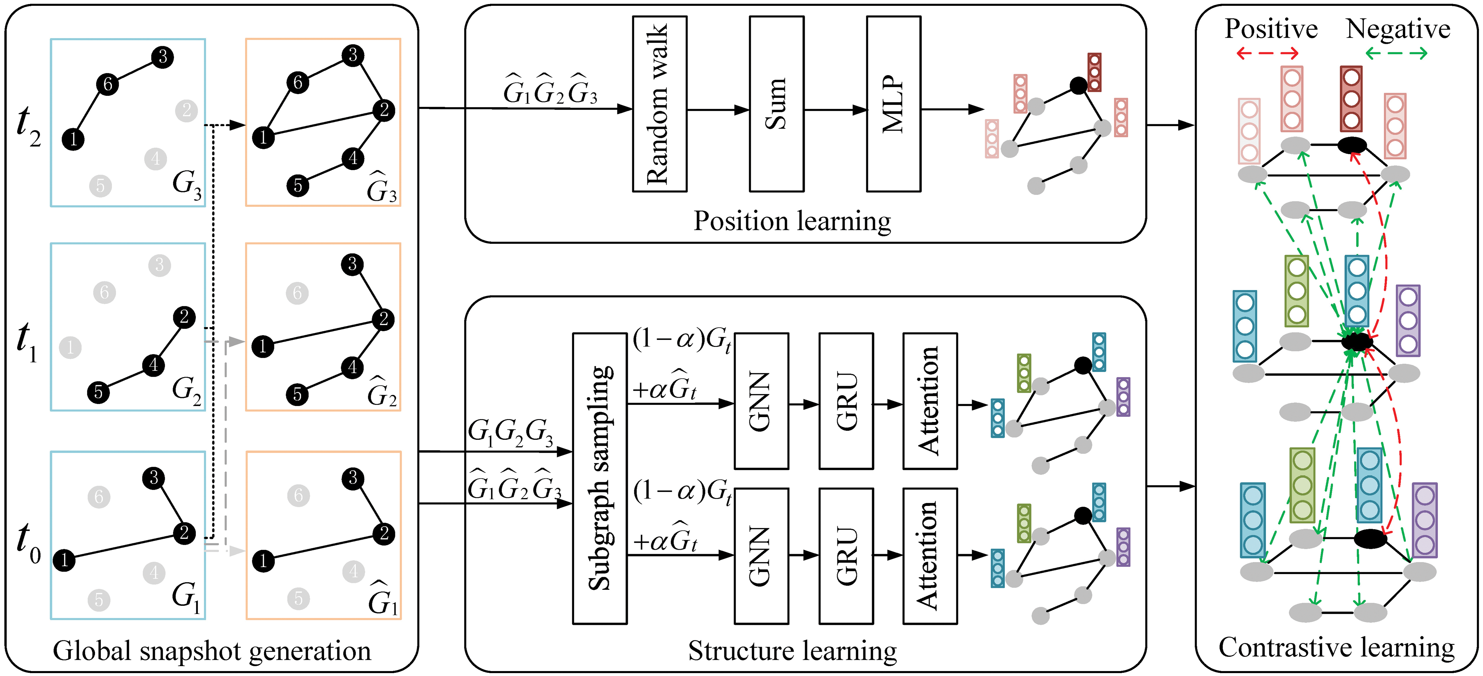
Figure 2: The framework of PSDGCL

3.2.1 Global Snapshot Generation Module

The global snapshot generation module aims to enhance the temporal information between snapshots and generate global snapshots as inputs to subsequent modules. Because each snapshot only records the interactions that occurred in the corresponding time slice, it is susceptible to random interference during data augmentation. To this end, a corresponding global snapshot is generated for each time slice based on the historical snapshot. Specifically, for time slice t, all node interactions up to time step t are obtained from the historical snapshots and recorded through the global snapshot G^t, which is computed as shown in Eq. (2):

A^t=∑n=1tAn(2)

where n denotes a time slice, An and A^t are the adjacency matrices of Gn and G^t, respectively.

In contrast, Gt contains the edges established within time slice t, while G^t records all edges established up to time slice t. That is, {G1,…,Gt,…,GT} expresses the short-term changes of the dynamic graph, while {G^1,…,G^t,…,G^T} expresses the long-term stable structure.

3.2.2 Position Learning Module

The position learning module aims to learn position-aware node features. Based on message passing, GNN makes it difficult to learn the positional information. As shown in Fig. 3, GNN performs message passing and aggregation based on the computational graph of each node. In this process, the same structure between Node 3 and Node C will result in the same representation. Meanwhile, although Nodes 2 and 3 are adjacent, different representations will be obtained due to different computational graphs, and they will be pushed away in the contrastive learning process. Therefore, node positions should be captured to learn the topology of the snapshot fully.

Figure 3: Message passing mechanism

Inspired by the characteristic of learning similar representations for adjacent nodes through random walks, we adopt random walks to capture approximate positional information. Specifically, random walks are first executed for each global snapshot, because the differences between global snapshots are small compared to snapshots. Then, the representations obtained from each global snapshot are added together, and the position representation Hp is generated through MLP. The complete calculation process is shown in Eq. (3).

Hp=MLP(∑tTRandomWalk(G^t))(3)

It is worth mentioning that we used all global snapshots instead of directly using the final global snapshot, in order to learn temporal information while capturing the positional information between nodes. For example, adjacent nodes in the final global snapshot may establish edges in different snapshots, the summation operation can make the learned representation more discriminative. Meanwhile, through MLP, the expressive power is enhanced without affecting the learned positional information, thus facilitating subsequent contrastive learning.

3.2.3 Structure Learning Module

The structure learning module aims to learn node representation from a structural perspective. First, the data augmentation method based on subgraph sampling is designed to generate two views. In order to better capture the evolving patterns of dynamic graphs, subgraphs are sampled from snapshots and global snapshots to capture short-term changes and long-term stable structures. Meanwhile, a hyperparameter α is added to control the sampling ratio. Assuming that the overall size of the subgraphs is M nodes, the sizes of subgraph sampled from snapshots and global snapshots are (1−α)M and αM nodes, respectively.

Secondly, combining GNN and GRU to learn corresponding node representations for each time slice. For a series of subgraphs sampled by node v in each view, taking time slice t as an example, the process of GNN aggregating messages of neighbor nodes to update the representation of central nodes is shown in Eqs. (4) and (5):

hv,t(k)=COMBINE(k)(hv,t(k−1),hn,t(k))(4)

hn,t(k)=AGGREGATION(k)({hi,t(k−1):i∈Nt(v)},{hi,t(k−1):i∈N^t(v)})(5)

where hv,t(k) is the k-th layer representation of the node v in the time slice t, especially hv,t(0)=xv,t. Nt(v) and N^t(v) denote the neighbor of node v in subgraph sampled from snapshot and global snapshot. In this paper, COMBINE(k) and AGGREGATION(k) are selected to sum and mean, respectively. After the L-layer calculation, the output of the GNN is denoted by {H1(L),…,Ht(L),…,HT(L)}, where Ht(L)={hv1,t(L)||…||hv|V|,t(L)} is the representation of all nodes of the time slice t corresponding to the snapshot.

GRU is used to learn the temporal features between snapshots. Taking Ht(L) as an example, the calculation process is shown in Eqs. (6)–(9):

rt=σ(WrHt(L)+Urht−1)(6)

zt=σ(WzHt(L)+Uzht−1)(7)

nt=tanh(WhHt(L)+rt⨀Uhht−1)(8)

ht=zt⨀ht−1+(1−zt)⨀nt(9)

where Wr and Ur, Wz and Uz, Wh and Uh are the weights of reset gate, update gate and tanh function, respectively, ht−1 is the hidden state of the previous moment, and ⨀ denotes the Hadamard product. The hidden state {h1,…,hT} of each time slice in GRU is used as the node representation after learning the temporal information.

Finally, based on {h1,…,hT}, the structure representation Hs is obtained through the attention mechanism for contrastive learning. The calculation process is as follows:

θ=softmax((hTWq)(HWk)Td)(10)

Hs=θ(HWv)(11)

where H={h1||…||hT}, Wq, Wk, Wv are trainable parameters, and d is the dimension of vector {h1,…,hT}. For the two different views generated, the results are recorded as Hs1 and Hs2.

3.2.4 Contrastive Learning Module

The contrastive learning module contrasts the representations learned by the above modules and optimizes the model while obtaining the final node representation. Specifically, firstly, for the representations Hs1 and Hs2 under the two views of the structure learning module, the representations from the same node are pulled closer, and the representations from different nodes are pushed away to learn the distinguishable structure representation. Taking the corresponding representation Hs1(v) and Hs2(v) of node v as an example, the following loss is adopted [19]:

ℒ1=−1|V|∑v∈Vlog⁡exp⁡(p(Hs1(v))Tp(Hs2(v))/τ)exp⁡(p(Hs1(v))Tp(Hs2(v))/τ)+∑u≠vexp⁡(p(Hs1(v))Tp(Hs2(u))/τ)(12)

where p(⋅) is the projection function of MLP, and τ is the temperature parameter.

Secondly, there should be a complementary relationship between the position representation and structure representation for the same node, so Hp is contrasted with the Hs1 or Hs2. Taking Hs1 as an example, the contrastive learning of Hp(v) and Hs1(v) for node v is as follows:

ℒ2=−1|V|∑v∈Vlog⁡exp⁡(p(Hs1(v))Tq(Hp(v))/τ)exp⁡(p(Hs1(v))Tq(Hp(v))/τ)+∑u≠vexp⁡(p(Hs1(v))Tq(Hp(u))/τ)(13)

where q(⋅) is a different projection function from p(⋅), because Hp and Hs1 are in different representation spaces. The total loss function is:

ℒ=βℒ1+(1−β)ℒ2(14)

Finally, Hs and Hp are concatenated to obtain the final node representation Z=[Hs,Hp].

4  Experiments

In order to verify the effectiveness of the model PSDGCL, experiments are designed to answer the following questions:

Question 1: Does PSDGCL outperform competing baselines?

Question 2: Are the critical components of PSDGCL helpful for improving the quality of learned representations?

Question 3: What are the impacts of hyperparameters on PSDGCL?

Question 4: How about the time complexity and space complexity of PSDGCL?

4.1 Datasets and Experiment Settings

4.1.1 Datasets

Table 1 shows the dataset used in the experiment, including bitcoin trading dataset Bitcoinotc, movie rating dataset ML1M, citation dataset DBLP, and tax transaction dataset TAX51.

4.1.2 Baselines

Six dynamic graph representation learning methods were selected as the baseline, including one supervised method and five unsupervised methods, in order:

1.    SpikeNet [14]: The supervised method combines GNN and SNN to learn the structural features and temporal features in the dynamic graph.

2.    MNCI [20]: Mining the influence of neighborhood and community, and updating the node embeddings after interaction through GRU.

3.    TGAT [21]: On the basis of a graph attention network, time information is incorporated through a time embedding function.

4.    EvolveGCN [10]: Modeling the evolution of GNN parameters through GRU to capture dynamics from the evolving parameters.

5.    HTGN [11]: Following the classic frameworks of GNN and GRU, hyperbolic space is introduced to capture the hierarchical structure of the network.

6.    HGWaveNet [12]: Diffusion convolution is used to increase the receptive field, and causal convolution is used to ensure that the temporal modeling order is not violated.

4.1.3 Implementation Details

The node classification task is used to verify the validity of the model. For the unsupervised method, after using graph reconstruction as a pretext task to obtain the node representation, a classifier is trained with 20% labels. For supervised methods, end-to-end models are trained using different proportions of labels under semi-supervised settings. For multi-classification tasks, the evaluation index selects Micro-F1 to consider the number of samples of different classes and adapt to the uneven distribution of classes.

4.2 Experiment 1: Comparative Experiment

For Question 1, Experiment 1 compares the performance of PSDGCL with each baseline. Table 2 shows the comparison results on the four datasets. It is worth noting that the supervised method SpikeNet uses different proportions of labels for training. The bolded results in the table are the optimal results, and the underlined results are sub-optimal results.

From Table 2, we can see that PSDGCL outperforms all baselines. In unsupervised methods, MNCI uses GRU to capture neighbor interactions, which performs worse than other GNN based methods. EvolveGCN uses GRU to model GNN parameter changes, which is more flexible but not as effective as directly learning temporal features. The HTGN based on hyperbolic space fully learns the hierarchical structure of nodes, which helps with node classification to some extent, while HGWaveNet perform poorly due to its focus on modeling edges. Although TGAT performs well, it uses graph reconstruction as the pretext task like the above methods, and the good performance in the graph reconstruction task is difficult to migrate to the node classification task. In contrast, PSDGCL takes into account the node structure and position through GCL, and achieves the best results in unsupervised methods. The supervised method SpikeNet benefits from the use of labels, outperforming most unsupervised methods when using 20% labels, and can continuously gain benefits as the proportion of label usage increases. When using the same number of labels, PSDGCL outperforms SpikeNet because all samples can be used for training based on GCL, while SpikeNet uses a much smaller number of labeled samples in a semi-supervised setting, which is particularly evident on large-scale datasets. In addition, PSDGCL has limited improvement on the ML1M dataset, possibly due to its smaller time scale and more frequent interactions between nodes.

4.3 Experiment 2: Ablation Experiment

For Question 2, Experiment 2 verifies the impact of different modules in PSDGCL on the results. To this end, two model variants, PSDGCL-RW and PSDGCL-AUG, are designed, which represent the removal of the position learning module and the removal of the global snapshot in the subgraph sampling. Fig. 4 shows the experimental results on different datasets.

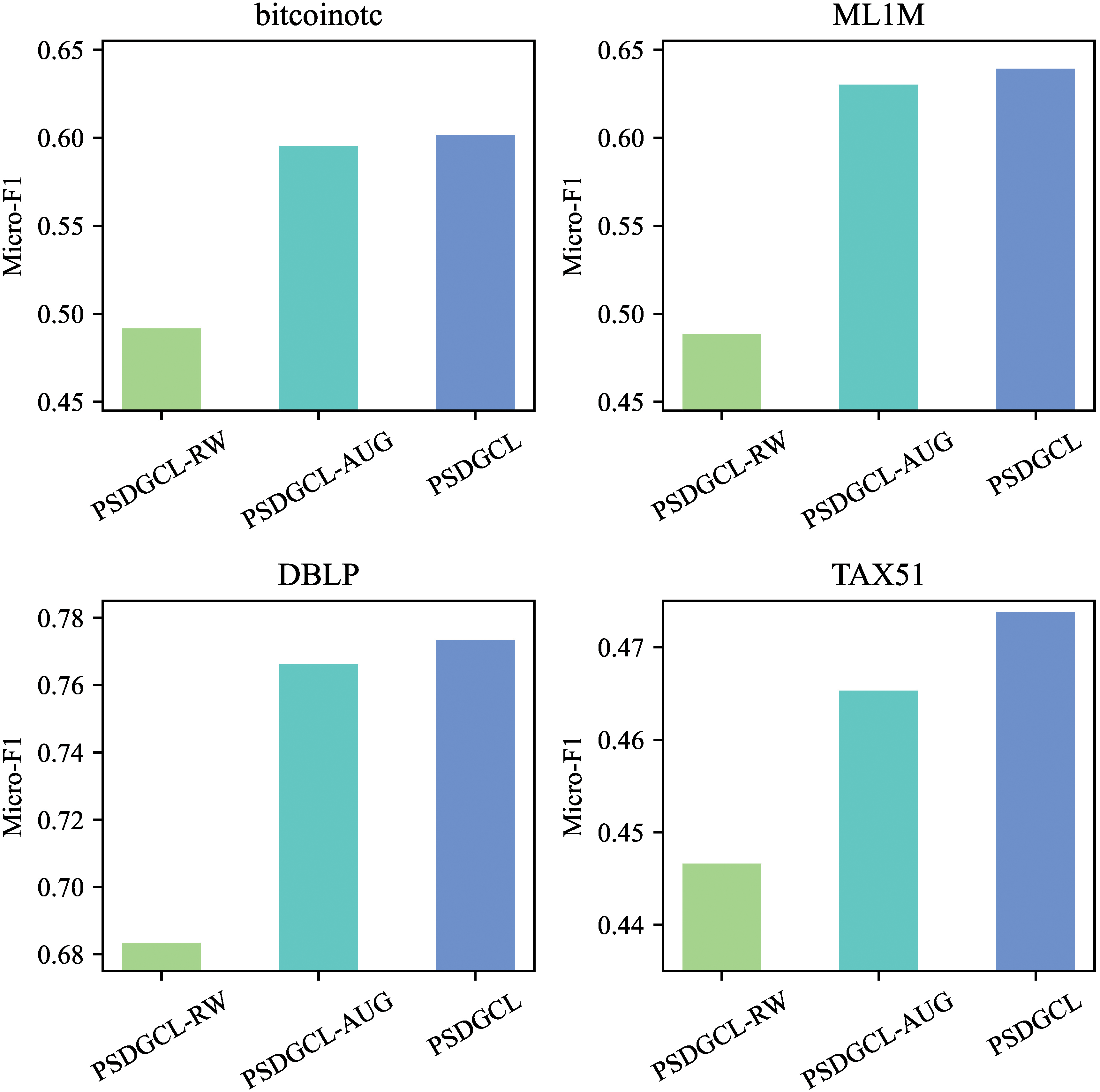
Figure 4: Ablation experiments

It can be seen from Fig. 4 that PSDGCL has the best performance because it comprehensively considers the structural information and positional information of nodes, and helps to capture the evolving pattern of dynamic graphs through global snapshots. Due to the differences in the characteristics of datasets, different modules have different effects on different datasets. Only by comprehensively considering all factors can a robust node representation be learned.

4.4 Experiment 3: Hyperparameter Experiment

For Question 3, Experiment 3 studies the performance of the model under different hyperparameters, including the sampling K-hop subgraphs, the sampling ratio α, and the loss weight β.

K-hop subgraph. The larger the sampled subgraph is, the more information is learned, but at the same time, more noise is introduced. Therefore, different subgraph sizes are sampled for experiments with different datasets. Considering the problem of space occupation and efficiency, we set K to {1, 2, 3}, and the experimental results are shown in Fig. 5.

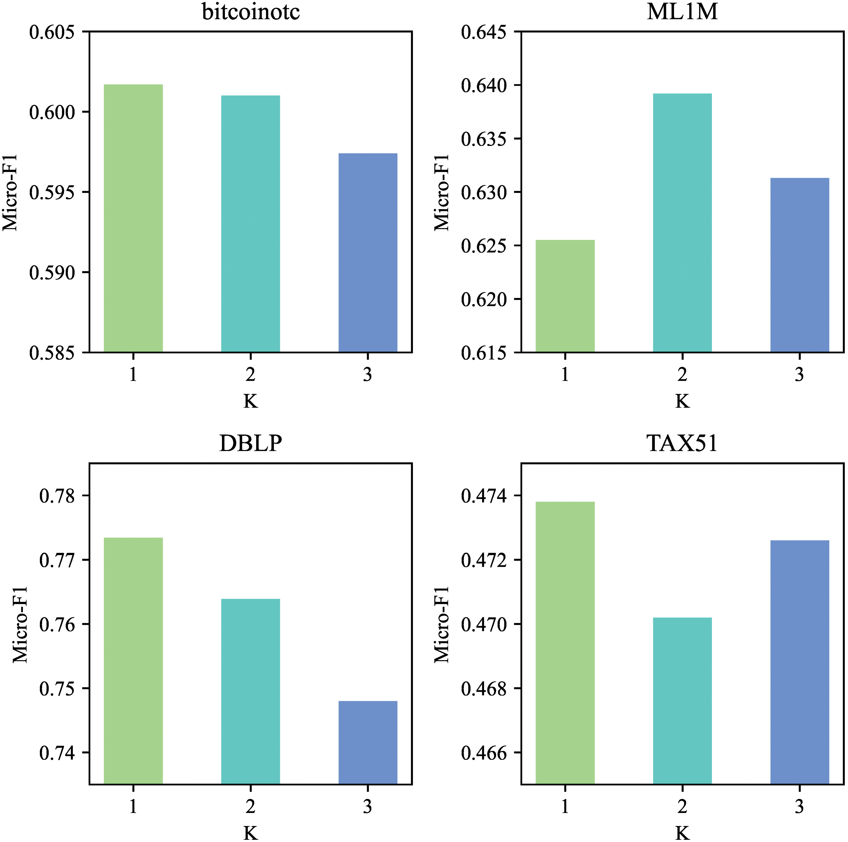
Figure 5: Analysis of subgraph size

From Fig. 5, it can be seen that subgraph size has a certain impact on performance, but it is not necessarily better to have a larger subgraph. Even a one-hop subgraph can often guarantee performance, which indicates that the node is closely related to its one-hop neighbors, and as the size of the subgraph increases, the risk of introducing noise also increases.

Sampling ratio α. The views generated by α control tend to learn more structural changes or more stable patterns to adapt to the characteristics of different types of data. The experimental results of the four datasets are shown in Fig. 6.

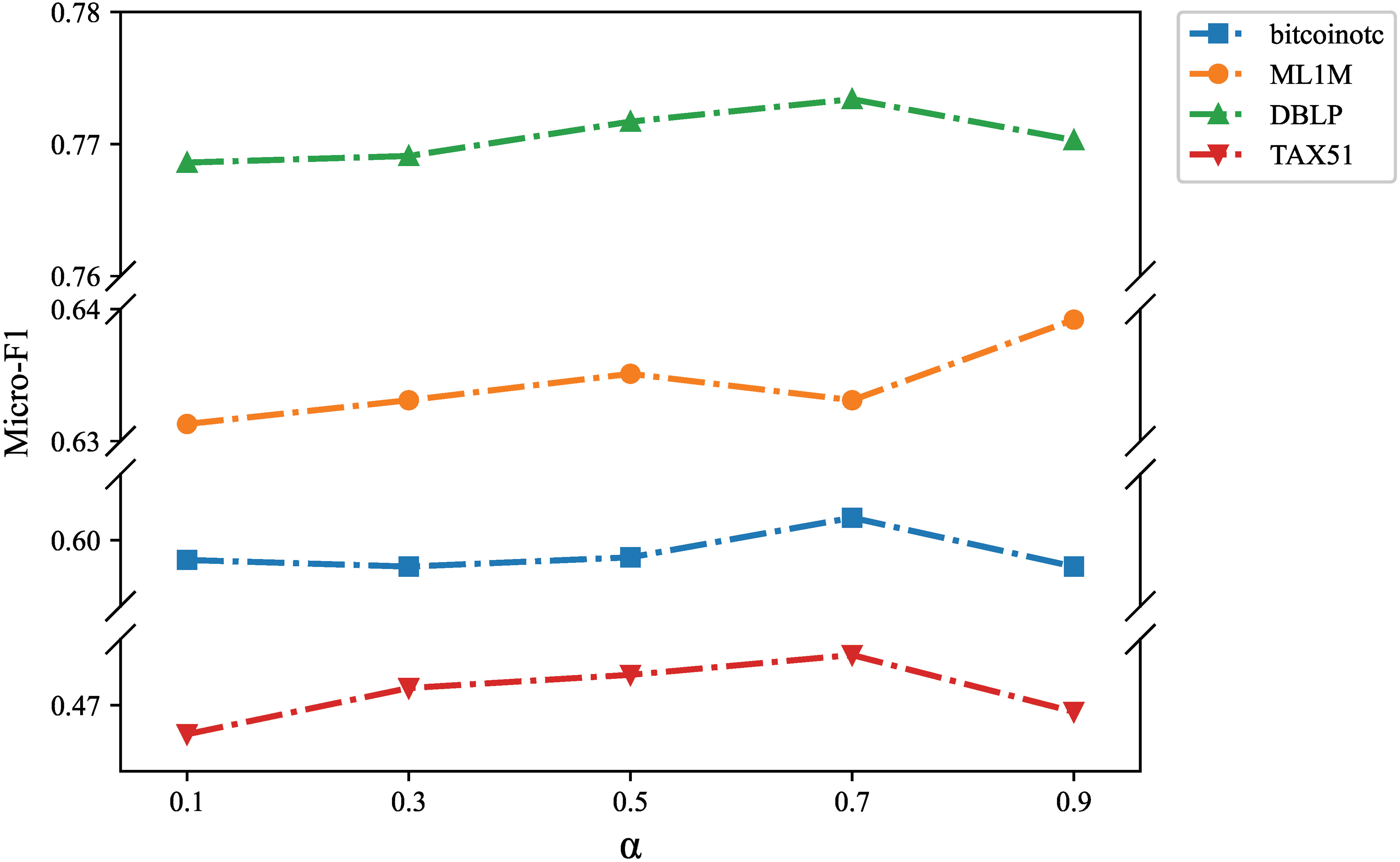
Figure 6: Analysis of sampling ratio

It can be seen that as α increases, the proportion of neighbors sampled from the global snapshot increases, and the performance often increases, which indicates that the global snapshot helps to learn the evolving pattern of the dynamic graph, thereby improving the quality of the learned representation. At the same time, α should not be too large, considering the short-term changes and long-term stable structure of the dynamic graph can better learn the evolving pattern.

Loss weight β. The hyperparameter β reflects the weights of two terms in the loss function. The larger the β is, the greater the impact of the contrast between the structural views on the model performance. On the contrary, it is necessary to contrast the structure representation and the position representation to learn the complementary information. The specific experimental results are shown in Fig. 7.

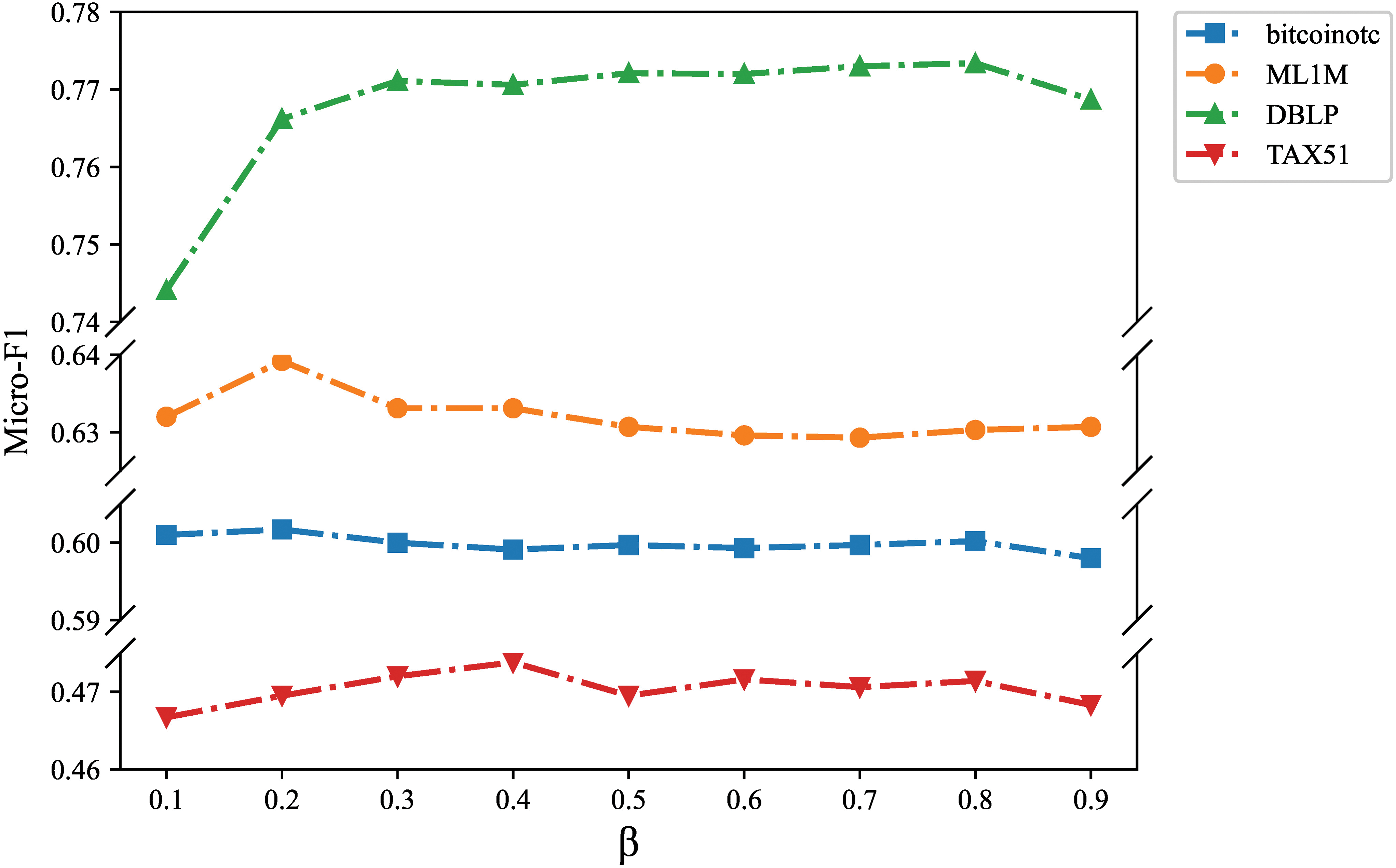
Figure 7: Analysis of loss weight

It can be seen that both terms in the loss function can help the model learn a better representation. The performance is often optimal when β reaches a small value, which indicates that the contrastive learning of structure representation and position representation can help learn complementary information to improve the quality of node representation.

4.5 Experiment 4: Complexity Experiment

For Question 4, Experiment 4 compares the time and space complexity of PSDGCL with baselines. In Table 3, we measure the time and space complexity by the model training time for each epoch (T) and the number of parameters (N), measured in seconds (s) and millions (M), respectively.

Table 3 shows that SpikeNet has the lowest complexity, which is due to the fact that semi-supervised learning only requires a few samples and the lightweight design of the model based on SNN. For unsupervised methods, the negative sampling process of contrastive learning makes PSDGCL have a higher time complexity, but this is acceptable compared to the performance improvement. Moreover, PSDGCL does not depend on complex model design and has space complexity second only to SpikeNet.

5  Conclusion

This paper proposes a new DGCL method PSDGCL, which is characterized by learning the structure and position of nodes at the same time to improve the quality of the learned node representation. Specifically, on the one hand, PSDGCL combines random walk and MLP to learn position-aware node representations. On the other hand, on the basis of using snapshots and global snapshots to express evolution patterns, PSDGCL uses subgraph sampling for data augmentation and combines GNN, GRU, and attention mechanisms to learn node structure. Finally, the model is optimized by GCL. Experimental results show that PSDGCL achieves comparable or even better performance than supervised learning methods without using labels.

In fact, PSDGCL still has limitations. Firstly, random walks can only capture fuzzy positional information. Secondly, how the time scale of dynamic graph affects the performance of the model is not clear. In the future, we will focus on finding more accurate position encoding methods and studying dynamic graphs at different time scales.

Acknowledgement: The authors are grateful to all the editors and anonymous reviewers for their comments and suggestions and thank all the members who have contributed to this work with us.

Funding Statement: The authors received no specific funding for this study.

Author Contributions: The authors confirm contribution to the paper as follows: study conception and design: Tian Liu; data collection: Tian Liu; analysis and interpretation of results: Tian Liu; draft manuscript preparation: Jian Feng, Tian Liu and Cailing Du. All authors reviewed the results and approved the final version of the manuscript.

Availability of Data and Materials: The data that support the findings of this study are available at https://github.com/LTIAN133/PSDGCL (accessed on 22 June 2024).

Ethics Approval: Not applicable.

Conflicts of Interest: The authors declare that they have no conflicts of interest to report regarding the present study.

References

1. Q. Chen, F. Jiang, X. Guo, J. Chen, K. Sha and Y. Wang, “Combine temporal information in session-based recommendation with graph neural networks,” Expert. Syst. Appl., vol. 238, Mar. 2024, Art. no. 121969. doi: 10.1016/j.eswa.2023.121969. [Google Scholar] [CrossRef]

2. W. Kong, Z. Guo, and Y. Liu, “Spatio-temporal pivotal graph neural networks for traffic flow forecasting,” presented at the 38th AAAI Conf. Artif. Intell. (AAAIVancouver, BC, Canada, Feb. 20–27, 2024, pp. 8627–8635. doi: 10.1609/aaai.v38i8.28707. [Google Scholar] [CrossRef]

3. H. Chen, P. Jiao, H. Tang, and H. Wu, “Temporal graph representation learning with adaptive augmentation contrastive,” presented at the Joint Eur. Conf. Mach. Learn. Knowl. Discov. Databases (ECML PKDDTurin, Italy, Sep. 18–22, 2023, pp. 683–699. doi: 10.1007/978-3-031-43415-0_40. [Google Scholar] [CrossRef]

4. J. Li, P. Bao, R. Yan, and H. Shen, “DyTSCL: Dynamic graph representation via tempo-structural contrastive learning,” Neurocomputing, vol. 556, Nov. 2023, Art. no. 126660. doi: 10.1016/j.neucom.2023.126660. [Google Scholar] [CrossRef]

5. P. Bao, J. Li, R. Yan, and Z. Liu, “Dynamic graph contrastive learning via maximize temporal consistency,” Pattern Recogn., vol. 148, Apr. 2024, Art. no. 110144. doi: 10.1016/j.patcog.2023.110144. [Google Scholar] [CrossRef]

6. L. Zhu, D. Guo, J. Yin, G. V. Steeg, and A. Galstyan, “Scalable temporal latent space inference for link prediction in dynamic social networks,” IEEE Trans. Know. Data. En., vol. 28, no. 10, pp. 2765–2777, Jul. 2016. doi: 10.1109/TKDE.2016.2591009. [Google Scholar] [CrossRef]

7. D. Rafailidis and A. Nanopoulos, “Modeling the dynamics of user preferences in coupled tensor factorization,” presented at the ACM Conf. Recomm. Syst. (RecSysSilicon Valley, CA, USA, Oct. 6–10, 2014, pp. 321–324. doi: 10.1145/2645710.2645758. [Google Scholar] [CrossRef]

8. S. D. Winter, T. Decuypere, S. Mitrović, B. Baesens, and J. D. Weerdt, “Combining temporal aspects of dynamic networks with Node2Vec for a more efficient dynamic link prediction,” presented at the IEEE/ACM Int. Conf. Adv. Soc. Netw. Anal. Min. (ASONAMBarcelona, Spain, Aug. 28–31, 2018, pp. 1234–1241. doi: 10.1109/asonam.2018.8508272. [Google Scholar] [CrossRef]

9. S. Mahdavi, S. Khoshraftar, and A. An, “dynnode2vec: Scalable dynamic network embeddingScalable dynamic network embedding,” presented at the IEEE Int. Conf. Big Data (Big DataSeattle, WA, USA, Dec. 10–13, 2018, pp. 3762–3765. doi: 10.1109/bigdata.2018.8621910. [Google Scholar] [CrossRef]

10. A. Pareja et al., “EvolveGCN: Evolving graph convolutional networks for dynamic graphs,” presented at the AAAI Conf. Artif. Intell. (AAAINew York, NY, USA, Feb. 7–12, 2020, pp. 5363–5370. doi: 10.1609/aaai.v34i04.5984. [Google Scholar] [CrossRef]

11. M. Yang, M. Zhou, M. Kalander, Z. Huang, and I. King, “Discrete-time temporal network embedding via implicit hierarchical learning in hyperbolic space,” presented at the 27th ACM SIGKDD Conf. Knowl. Discov. Data Min. (KDDSingapore, Aug. 14–18, 2021, pp. 1975–1985. doi: 10.1145/3447548.3467422. [Google Scholar] [CrossRef]

12. Q. Bai, C. Nie, H. Zhang, D. Zhao, and X. Yuan, “HGWaveNet: A hyperbolic graph neural network for temporal link prediction,” presented at the ACM Web Conf. 2023 (WWWAustin, TX, USA, Apr. 30–May 4, 2023, pp. 523–532. doi: 10.1145/3543507.3583455. [Google Scholar] [CrossRef]

13. H. Li, Z. Zhang, D. Liang, and Y. Jiang, “K-Truss based temporal graph convolutional network for dynamic graphs,” presented at the Asian Conf. Mach. Learn. (ACMLHanoi, Vietnam, Dec. 5–8, 2024, pp. 739–754. [Google Scholar]

14. J. Li et al., “Scaling up dynamic graph representation learning via spiking neural networks,” presented at the 37th AAAI Conf. Artif. Intell. (AAAIWashington, DC, USA, Feb. 7–13, 2023, pp. 8588–8596. doi: 10.1609/aaai.v37i7.26034. [Google Scholar] [CrossRef]

15. N. Yin et al., “Dynamic spiking graph neural networks,” presented at the 38th AAAI Conf. Artif. Intell. (AAAIVancouver, BC, Canada, Feb. 20–27, 2024, pp. 16495–16503. doi: 10.1609/aaai.v38i15.29587. [Google Scholar] [CrossRef]

16. X. Qin, N. Sheikh, C. Lei, B. Reinwald, and G. Domeniconi, “SEIGN: A simple and efficient graph neural network for large dynamic graphs,” presented at the 39th Int. Conf. Data Eng. (ICDEAnaheim, CA, USA, Apr. 3–7, 2023, pp. 2850–2863. doi: 10.1109/icde55515.2023.00218. [Google Scholar] [CrossRef]

17. K. Zhao and L. Zhang, “Causality-inspired spatial-temporal explanations for dynamic graph neural networks,” presented at the 12th Int. Conf. Learn. Represent. (ICLRVienna, Austria, May. 7–11, 2024. [Google Scholar]

18. J. Chen and G. Kou, “Attribute and structure preserving graph contrastive learning,” presented at the 37th AAAI Conf. Artif. Intell. (AAAIWashington, DC, USA, Feb. 7–13, 2023, pp. 7024–7032. doi: 10.1609/aaai.v37i6.25858. [Google Scholar] [CrossRef]

19. T. Chen, S. Kornblith, M. Norouzi, and G. Hinton, “A simple framework for contrastive learning of visual representations,” presented at the 37th Int. Conf. Mach. Learn. (ICMLVienna, Austria, Jul. 13–18, 2020, pp. 1597–1607. doi: 10.48550/arXiv.2002.05709. [Google Scholar] [CrossRef]

20. M. Liu and Y. Liu, “Inductive representation learning in temporal networks via mining neighborhood and community influences,” presented at the Int. ACM SIGIR Conf. Res. Dev. Inf. Retr. (SIGIRCanada, Jul. 11–15, 2021, pp. 2202–2206. doi: 10.1145/3404835.3463052. [Google Scholar] [CrossRef]

21. D. Xu, C. Ruan, E. Korpeoglu, S. Kumar, and K. Achan, “Inductive representation learning on temporal graphs,” presented at the 8th Int. Conf. Learn. Represent. (ICLRAddis Ababa, Ethiopia, Apr. 26–30, 2020. doi: 10.48550/arXiv.2002.07962. [Google Scholar] [CrossRef]