A Combined Method of Temporal Convolutional Mechanism and Wavelet Decomposition for State Estimation of Photovoltaic Power Plants

1  Introduction

As new energy develops, photovoltaic power is increasingly utilized. However, photovoltaic power generation varies with daily solar irradiance, and stations are typically scattered, unlike centralized thermal power plants. Thus, regulating photovoltaic power stations is crucial.

State estimation, key to power system awareness, impacts plant control effectiveness. Power state estimation methods fall into three main categories: transmission-based, distributed-based, and pseudo-measurements [1]. Supervisory control and data acquisition (SCADA) and phasor measurement units (PMUs) are commonly used for transmission-based methods. The SCADA system [2] integrates RTU, communication networks, a main station, and interactive interfaces to provide asynchronous data every 2–5 s. PMUs [3] offer voltage and current phasor measurements with timestamps via high-precision GPS, reporting 50–60 times per second. Besides SCADA and PMU’s distributed applications, AMI [4,5] holds significant potential for state estimation in distributed systems. Advanced metering infrastructure (AMI) includes smart meters, data concentrators, communication networks, and data management systems. Smart meters can capture samples at rates up to 30 Hz. However, AMI submits locally stored data to remote databases only once or twice daily. Pseudo measurements address unobservability and enhance measurement redundancy, which are categorized into statistical and learning-based types. Statistical measurements necessitate separate modeling for various data sources, incurring high costs, while learning-based methods enhance model universality by not requiring separate data modeling.

Currently, learning-based pseudo measurements evolve with the advancement of deep learning. Common methods are clustering, artificial neural networks, and probabilistic neural networks. These methods aim to minimize the gap between predicted and actual values. This paper introduces the RST-LSTM framework, featuring load decomposition for high-frequency data extraction and an enhanced recurrent neural network for training and testing. The framework addresses long-sequence feature extraction, enhances prediction accuracy, and offers more reliable pseudo-measurement data for state recognition.

The remaining structure of this article is as follows: Section 2 reviews related work; Section 3 details the proposed RST-LSTM framework; Section 4 discusses comparative and ablation study results; Section 5 concludes the paper.

2  Related Work

2.1 Power Plant State Estimation Based on Pseudo Measurements

The current pseudo measurement based power plant state estimation is mainly based on learning. Reference [6] proposed a new high-precision photovoltaic power generation prediction model. This method preprocessed photovoltaic power generation data before model training, including weather type classification, similar day selection, and principal component analysis. Genetic algorithms were also employed to optimize the initial weights and thresholds during training. The experimental results demonstrated the significance of weight setting in accurately detecting and identifying bad data. Reference [7] proposed a consumer fit distribution determination method based on probabilistic neural network (PNN). This method used wavelet multi-resolution analysis based on actual load profile data and introduced fuzzy c-means (FCM) clustering algorithm. The experimental results indicated that this method can identify consumers who deviate from the contract schedule, offering management solutions for the power industry. Reference [8] proposed a new method to predict the load distribution of low-power customers in low-voltage distribution networks. This method was divided into two stages. The first stage proposed a frequency based clustering algorithm to extract user load patterns, which had superior performance compared to commonly used methods such as K-means. The second stage proposed a total load data prediction method, which can forecast load data two weeks ahead, using historical energy consumption data and sample customer data.

2.2 Load Data Decomposition

Load Decomposition [9] is a method that decomposes the original load signal into multiple sub-signals to optimize feature extraction. Currently, wave form decomposition methods are widely used to solve load decomposition problems. The commonly used decomposition methods are Empirical Mode Decomposition (EMD) [10], Variational Mode Decomposition (VMD) [11], and Wavelet Decomposition (WD) [12]. The EMD method decomposes the data based on its own time scale characteristics, which means that the method does not need to set any basis functions in advance. Theoretically, it can be used to decompose any feature signal, and the resulting sub-signals are stationary signals. The VMD method uses an iterative search for the optimal solution of the variational model, which determines the center frequency and bandwidth of each decomposed component. Each mode is smooth after demodulation into the baseband. Compared to the EMD method, the number of components obtained by the VMD method is determined, and the VMD method can suppress the mode mixing phenomenon of the EMD method. The Wavelet decomposition method, its process is to decompose the original signal into approximate coefficient signals and detail coefficient signals, and then decompose the approximate coefficient signals into the next layer set. The approximate coefficient signal corresponds to a low-frequency signal, while the detail coefficient signal corresponds to a high-frequency signal. Using the Wavelet method, the original signal can be denoised to obtain a smoother data signal.

2.3 Load Forecasting Based on Recurrent Neural Networks

Currently, the most commonly used recurrent neural networks are long short term memory network (LSTM) [13,14], gated recurrent unit (GRU) [15,16] and dual stage attention based recurrent neural network (DA-RNN) [17]. Recurrent neural networks [18] are capable of transmitting past time information within cells, which makes them suitable for processing time series data. For LSTM networks, the recurrent unit consists of several gating mechanisms, including forget gate, input gate, and output gate. The forget gate decides which information to pass on and which to discard. For GRU, it includes only two gating mechanisms: update gate and reset gate. Compared to LSTM, the simplification speeds up training time but may slightly compromise accuracy. Compared to the first two, DA-RNN introduces and improves attention mechanism. The role of attention mechanism is to allocate weights, which makes the model focus on specific inputs. DA-RNN uses two stages of attention mechanism [19] to optimize recurrent neural networks. In the first stage, adaptive feature extraction is performed on the input by referring to the hidden state of the encoder. The second stage selects hidden states for all time steps through attention mechanism. This two-stage attention mechanism optimizes the feature extraction performance of recurrent neural networks for long time series.

3  Methodology

3.1 Structure of RST-LSTM

RST-LSTM model is based on time convolutional network (TCN), LSTM model, self-attention mechanism, and reinforcement output activation unit, as depicted in Fig. 1. RST-LSTM obtains the local feature information Yi′ of the input data Xi, using the basic module ST-LSTM. Subsequently, the input data is connected to the output data of each stacked temporal convolutional memory unit Module (ST-LSTM) layer, using an improved residual network connection method. After the combination with the enhanced output activation unit, the final predicted output Yi is obtained.

Figure 1: Structure of RST-LSTM

Time series prediction predicts the next step of load data by utilizing historical time data. The feature learning effect of the model on the input sequence directly affects the accuracy of the output sequence. Therefore, ST-LSTM is developed to enhance LSTM, which improve fundamental feature extraction. The input data is processed through a time convolutional network to obtain global sequence information. Compared to traditional convolutional neural networks, time convolutional networks can extract features from sequences of any step size. Then, local feature learning is carried out through the LSTM module, and a self attention mechanism is added at the output end to enhance some feature information. Compared to a simple progressive network structure, dense convolutional networks are used for optimization and combination. The input sequence is subjected to multi-layer feature analysis by the ST-LSTM, deriving preliminary insights. On this basis, an improved residual network is used to connect the outputs of each layer of ST-LSTM, reducing the use of stacking modes and model redundancy.

3.2 Load Data Preprocessing Strategy Based on Wavelet Decomposition

Wavelet decomposition is an indispensable method in signal processing and analysis. Compared to traditional Fourier transform methods, wavelet decomposition is more stable and performs better in signal processing. Considering that both signal data and load power data are time series, wavelet decomposition preprocessing is applied to load data to reduce prediction errors. This paper introduces wavelet decomposition to preprocess the input load data.

The original input data is decomposed into a triple sequence through wavelet decomposition. They are the first layer of low-frequency data, the first layer of high-frequency data, and the second layer of high-frequency data. Then, input the obtained low-frequency data and high-frequency data into the RST-LSTM prediction module for prediction analysis. Finally, the predicted values corresponding to low-frequency and high-frequency data are reconstructed, using wavelet transform to obtain the final predicted data.

Among them, wavelet decomposition can be divided into continuous wavelet decomposition and discrete wavelet decomposition. For any input data signal g(x), its continuous wavelet decomposition equation is:

CWTφg(m,n)=∫−∞+∞g(x)φ¯m,n(x)dx=m−12∫−∞+∞g(x)φ¯(t−nm)dx(1)

where m and n are scale parameters and positional parameters, respectively. φ¯(t) represents the complex conjugate form of φ(t). The overall continuous wavelet decomposition is manifested as the similarity between input data signal g(x) and φm,n(x). In the process of continuous wavelet decomposition, the wavelet coefficients are determined by the continuous expansion wavelet and the shifted mother wavelet, so all possible scale and time wavelet coefficients can be calculated.

3.3 Stacked Temporal Convolutional Memory Unit

Although LSTM has obvious advantages for short sequences, there are still drawbacks such as gradient explosion and vanishing when it comes to the demand for long sequences. In addition, excessive linear stacking of LSTM not only greatly increases the time loss of the model, but also generates high redundancy of the model, greatly reducing prediction accuracy. Therefore, the stacked temporal convolutional memory unit module integrates the Time Convolutional Network (TCN) module, LSTM model and self-attention mechanism. By adopting the connection approach of denseness, it simplifies the transmission mode of linear overlay LSTM, which reduces time loss, and improves the ability of model feature analysis. The design of the stacked temporal convolutional memory unit is shown in Fig. 2.

Figure 2: Structure of the stacked temporal convolutional memory unit

3.3.1 Time Convolutional Network Dilation Mechanism

Recurrent neural networks (RNNs) have excellent performance in time series processing. However, RNN also has relative limitations. When it comes to long sequences, the model’s complexity and memory requirements can increase significantly. How to reduce complexity without affecting the efficiency of feature extraction has become a problem to be solved. Therefore, Bai et al. [20] combined the ideas of dilated convolution and residual networks to construct a Time Convolutional Network (TCN) in 2016. Compared to traditional RNN processing methods, TCN utilizes its own convolutional layer when processing time series, which can parallelly process relevant data and reduce time loss. Meanwhile, combining the idea of dilated convolution, different input and output requirements can be adjusted by changing the size of the receptive field. Finally, by combining the residual network connection method, the drawbacks of gradient explosion and vanishing are effectively avoided [21–23]. Fig. 3 is the schematic diagram of a time convolutional network. The use of dilated convolution in TCN can better match the feature extraction of relevant sequences. The output expression of dilated convolution is: G(F,X)=(F∗X)xi=∑k=1Nfkxt−(N−k)d, the input sequence is X={x0,x1,x2,…,xn}; The expression for the corresponding convolution kernel of size N is F={f1,f2,f3,…,fN}; fk is the number of filters in the corresponding convolution operation, d is the dilation factor. In order to increase the stability of convolutional networks, residual networks are introduced to reduce gradient vanishing and exploding phenomena caused by excessively long sequences. The input data is overlaid with the data from the previous output layer through a 1 × 1 convolution operation to obtain the final output data.

Figure 3: Structure of time convolutional network

3.3.2 Self Attention Reinforcement Mechanism

The self attention reinforcement mechanism is an optimization model based on the attention mechanism. The attention mechanism focuses on the correlation between data inputs and optimizes the model’s high dependence on data.

The self attention reinforcement mechanism uses the self attention mechanism as the main component module. The self attention mechanism can improve the correlation between internal features of data, reduce the model’s external dependence on data, and achieve the model’s own data loop. The essence of self attention mechanism is to calculate the mutual influence relationship between each input data and obtain the long-term dependencies. The structure of the self attention mechanism is shown in Fig. 4.

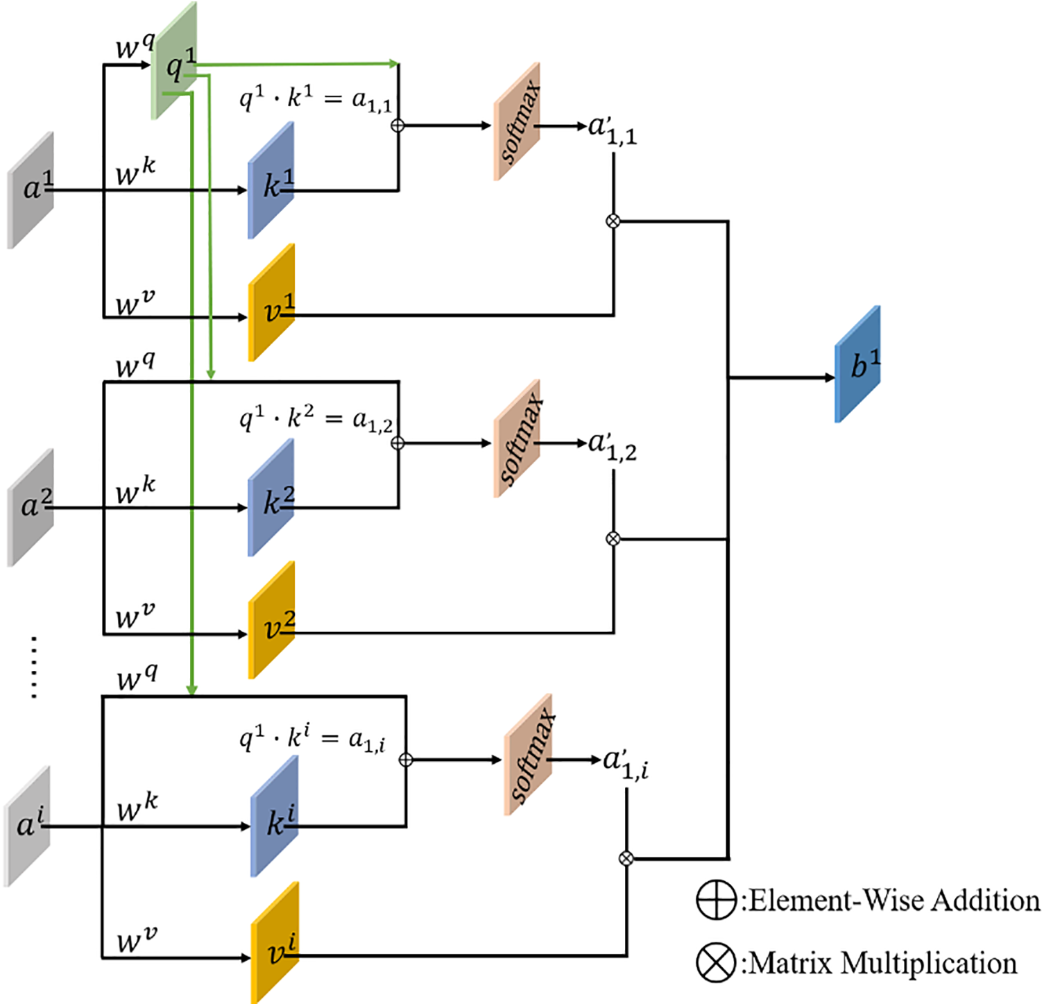
Figure 4: Structure of self attention mechanism

Firstly, perform different convolution operation on the input data wq, wk, wv, and obtain the corresponding value of q, k, v. The first round of convolution operation shares the first q value globally, called q1, convolved with different k values, and the corresponding score value a1,i′ is obtained through the softmax function. The obtained a1,i′ perform a product operation with the corresponding vi, and finally accumulate all the product operations to obtain the weighted sum value b1 for q1.

In addition, drawing on the connection method of Densnet, skip connections are made between the input data before the first layer of long short memory module and the data between the long short memory module, which is based on the linear connected time convolutional network, long short memory module, and self attention mechanism, strengthening the self attention mechanism’s analysis of the correlation between internal features of the data. On the basis of reducing the superposition of linear networks, the feature analysis ability is improved, and the prediction accuracy of the entire ST-LSTM is optimized. The internal transfer output of the ST-LSTM model is shown in formula:

yi=xi||LSTMi||LSTMi+1||F(xi)(2)

Among it, yi is the final output, xi is the current input data, LSTMi is the transfer output of the current long short memery module, and LSTMi+1 is the transfer output of the next layer of long short memory module. F(xi) is the transfer output of the overall feature extraction module, and || represents the superimposed combined output. The enhanced skip combination method not only reduces the drawbacks of model redundancy caused by the multi-layer stacking of LSTM, but also increases the global receptive field of ST-LSTM, improving the accuracy of the model in feature analysis.

3.4 Residual Combination Optimization Structure

The residual combination optimization structure draws inspiration from the ideas of multi-level residual network (MRN) to reduce network redundancy and gradient explosion caused by network stacking.

Among them, MRN uses the idea of convolutional connections to enhance the convolutional outputs of each layer. While ST-LSTM focuses on extracting time series features, MRN focuses on the convolutional outputs of various interval values in the input data and intermediate network layer output data, and enhances the outputs by combining various activation functions. Partial skip connections are achieved through residual networks to increase the receptive field information of the model, improving overall prediction accuracy. The overall process of residual combination optimization structure is shown in Fig. 5.

Figure 5: Structure of residual combination optimization

The transfer process of residual combination optimization structure is shown in formula:

yi=xi||Act(xi)||Act(Model1)||Model1||Act(Model2)||F(xi)(3)

yi is the final output, xi is the current input data, Modeli is the output passed by the ith layer model, F(xi) represents the transfer output of the overall feature extraction module, and || represents the superimposed combined output, Act(i) is the convolutional transfer function. Compared to the linear superposition of multi-layer convolutional networks, the residual combination optimization structure uses convolutional transfer functions to connect the outputs between different layers of models, skipping the transfer of part of the output data. The structure improves the accuracy of feature extraction only through multi-layer connections, without adding additional parameters, meeting the demands for both timely response and accurate forecasting.

Drawing inspiration from the one-dimensional CNN convolutional output mode in MRN, the residual combination optimization structure also utilizes the enhanced convolutional connection mode to activate various transfer outputs. Compared to using a single Relu activation function, the enhanced convolutional connection mode uses a combination of Softmax and Relu functions to activate the output. The softmax function is suitable for multi-classification problems and can effectively aggregate and classify various similar features. The load data is first convolved and classified by using 1D CNN, and then output by using Relu function, effectively improving the accuracy of various feature analysis and thus improving prediction accuracy.

4  Experiment Evaluation

4.1 Evaluation Indicators

Time series prediction is mainly aimed at predicting the relevant step sizes of input sequence, and the main evaluation parameters include accuracy indicators. The accuracy indicators, with r2 as the main indicator, reflects the fitting effect of the model and the accuracy of the model during prediction. The specific calculation formula is as follows:

r2=1−∑i=1k(zi−zi^)2∑i=1k(zi−z¯)2(4)

zi represents the predicted value information output, z^i represents the true value information of the input, z¯ represents the average value information of the input value. k represents a total of k sample information data. The larger r2, the better the fitting effect of the model, and the higher the prediction accuracy. In addition, for short-term load forecasting, time loss is also an essential testing indicator, and the time loss indicator used in this paper is cost_avg_Epoach. The relevant expression is as follows:

costAvgEpoach=∑i−1ncostTimen(5)

n represents the maximum number of iterations in the network, which is set to 100 by default in this experiment. cost_Time represents the time consumed by the model during each training round. At the same time, in order to comprehensively verify the stability of the model and the accuracy of the prediction effect, RMSE and MAE are also used as additional evaluation indicators. The relevant expressions are as follows:

RMSE=1k∑i=1k(zi−z^i)2(6)

MAE=1k∑i=1k|zi−z^i|(7)

zi represents the predicted value information output, z^i represents the true information of the input. k represents a total of k sample information data.

4.2 Results of Comparative Experiments

This section compares five comparative models: LSTM, GRU, CNN-LSTM, LSTNet, DARNN, and the Short Term Load Forecasting Method (RST-LSTM) proposed in this paper. The models for comparison and the model proposed in this paper all used the same test and training sets. The various comparative experimental results obtained are shown in Table 1.

In Table 1, based on the electricity load data of Anhui Province in 2022, RST-LSTM has significant advantages in various indicators. Among the six types of models, RST-LSTM achieved the highest scores on r2 cost_avg_Epoach, RMSE, and MAE.

Among the six types of networks, the stacked GRU model and the stacked LSTM model, although achieving better performance in single time loss, have the worst performance on the r2 indicator. And, as the model layers are stacked, there will be phenomena of gradient explosion, which leads to a loss of accuracy in the model. LSTNet is essentially an optimized combination network of convolutional layers and LSTM, but it introduces an autoregressive structure and attention mechanism, resulting in high time loss of the model. Compared to LSTNet and stacked LSTM models, CNN-LSTM is still relatively excellent in the r2 and cost_ave_Epoach. In CNN-LSTM, the linear stacking network of convolutional layers and LSTM effectively reduces the gradient explosion phenomenon in stacked LSTM, but the time loss also increases. DARNN model is essentially a recurrent neural network with a two-stage attention mechanism, which has high accuracy in the r2, increasing by 30.4% compared to LSTM. However, it also has the highest time loss. Based on the advantages of different models which are mentioned above, the prediction results of some time periods are selected for comparison. The results are shown in Fig. 6. The time interval on the horizontal axis is 2 h, and the unit on the vertical axis is 103.

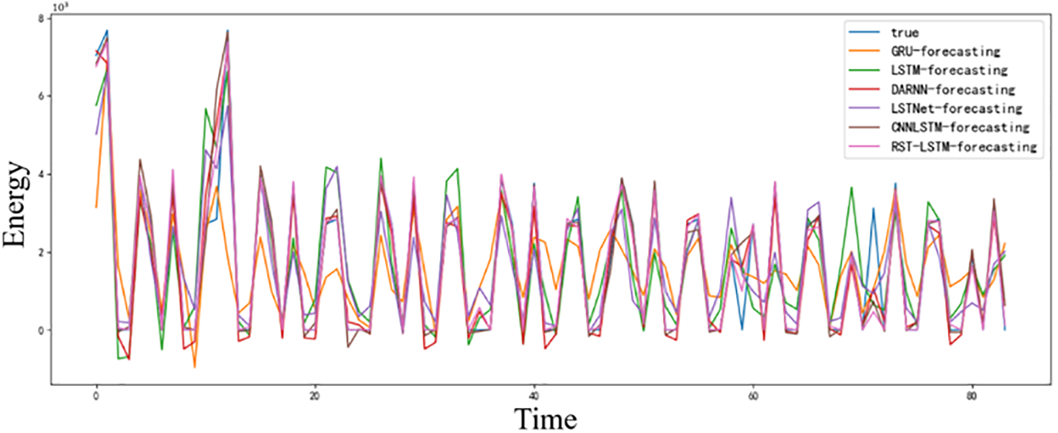
Figure 6: Load forecasting results of 6 types of models

In Fig. 6, different colors are used to represent the predictive performance of different prediction models. Among them, the light pink RST-LSTM stands out with the top predictive performance, and the predictions of other models also vary. However, for local feature extraction, especially for zero value prediction, RST-LSTM’s activation function based on Softmax Relu can effectively classify features and improve the prediction accuracy of salient features. Therefore, in terms of local prediction, RST-LSTM can still maintain high predictive performance. LSTNet, LSTM and GRU cannot efficiently analyze the overall features due to their various properties and the drawbacks caused by excessive stacking. Overall, RST-LSTM is the best in terms of time loss and prediction accuracy.

4.3 Results of Ablation Experiments

In order to verify the effectiveness of the RST-LSTM model and residual combination optimization structure, this paper conducts relevant ablation experiments based on the 2022 Anhui Province power load dataset. The experimental results are shown in Table 2 and Fig. 7. LSTM-5 represents a 5-layer stacked LSTM network model, R-LSTM-2 represents a two-layer LSTM model using residual combination optimization structure, ST-LSTM represents a load forecasting model that removes residual combination optimization structures and adopts a stacked form.

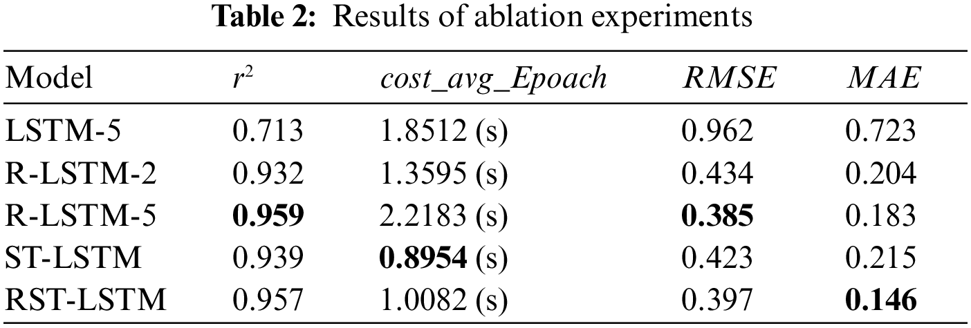
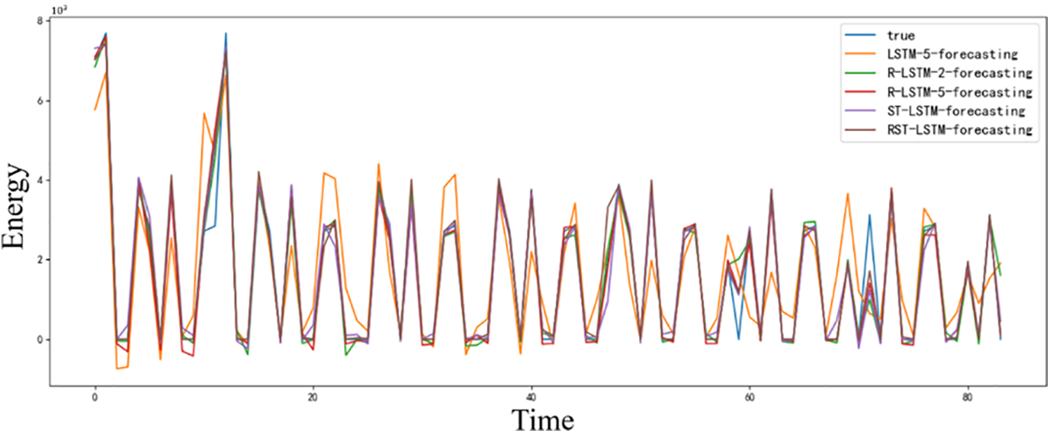
Figure 7: Results of ablation experiments

Specifically, when removing residual combination optimization structures, compared to RST-LSTM, the single time loss of ST-LSTM has decreased by 0.1128 s. However, the r2 indicator decreased by 1.8%. This indicates that the residual combination optimization structure has improved the prediction accuracy of the model while sacrificing some time. Comparing R-LSTM-2 and RST-LSTM, they all adopt a two-layer model based on residual combination optimization structure. Compared to LSTM, ST-LSTM showed an improvement in both single time loss and r2 index, with a decrease of 0.3513 s and an increase of 2.5%, respectively. This indicates that the proposed stacked temporal convolutional memory unit Module (ST-LSTM) performs better than LSTM on the 2022 Anhui Province power load dataset. Finally, comparing LSTM-5 and R-LSTM-5, it can be seen that in the case of 5-layer LSTM stacking, the model has the drawback of gradient vanishing, and the r2 indicator has significantly decreased. However, the 5-layer LSTM stacking model based on residual combination optimization structure can maintain a high level of r2 index. This reflects that residual combination optimization structure helps alleviate the phenomenon of gradient vanishing caused by too many stacked models.

In order to verify the effectiveness of the enhanced convolutional connection activation function, this paper also compared various commonly used activation functions on the same model and dataset. The results are shown in Table 3, Figs. 8 and 9.

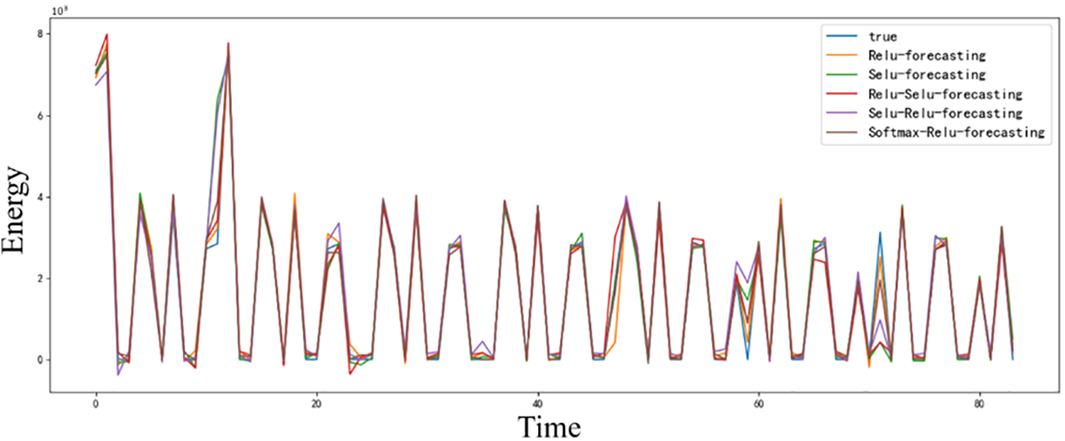
Figure 8: Results of ablation experiments

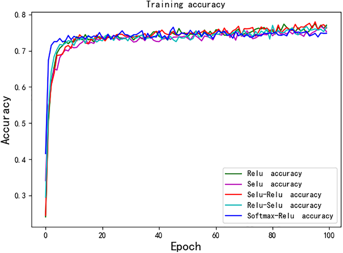
Figure 9: Process of training

As shown in Table 3, the combination of Softmax Relu has the worst single time loss and the best performance in other indicators. However, there is a difference of 0.0559 s between the single time loss and the optimal Relu activation function, and the r2 indicator has increased by 4.5%. Therefore, although the Softmax activation function has some time loss in classification problems, it has a high improvement in model accuracy. Meanwhile, in Fig. 8, the combination of Softmax Relu has the best performance in predicting zero values and partial feature values. Finally, as shown in Fig. 9, the combination of Softmax Relu has the highest initial value and fastest convergence of the model in the first 10 iterations. Therefore, for short-term load forecasting which requires low time loss and high accuracy, the combination of Softmax Relu is feasible.

5  Conclusion

This paper proposes a new deep learning framework for State Estimation of Photovoltaic Power Plants. By combining stacked memory modules and wavelet decomposition strategies, the framework enhances local feature extraction and can focus on global feature analysis. Meanwhile, RST-LSTM has achieved the best prediction performance among the six types of load forecasting models, and can also maintain high accuracy in local forecasting, based on the electricity load data of Anhui Province in 2022. In addition, the effectiveness of the residual combination optimization structure proposed in this paper was verified through ablation experiments on residual structures, providing a more accurate solution for power plant state estimation based on pseudo measurements.

Acknowledgement: The authors would like to express their gratitude to the editors of this article.

Funding Statement: This research was funded by NARI Group’s Independent Project of China (Granted No. 524609230125) and the foundation of NARI-TECH Nanjing Control System Ltd. of China (Granted No. 0914202403120020).

Author Contributions: The authors confirm contribution to the paper as follows: study conception and design: Shaoxiong Wu, Ruoxin Li; data collection: Hailong Wu; analysis and interpretation of results: Xiaofeng Tao, Ping Miao, Qi Liu; draft manuscript preparation: Yang Lu, Yanyan Lu, Li Pan. All authors reviewed the results and approved the final version of the manuscript.

Availability of Data and Materials: This data is self processed by the authors, so it is unavailable.

Ethics Approval: Not applicable.

Conflicts of Interest: The authors declare that they have no conflicts of interest to report regarding the present study.

References

1. G. Cheng, Y. Lin, A. Abur, A. Gómez-Expósito, and W. Wu, “A survey of power system state estimation using multiple data sources: PMUs, SCADA, AMI, and beyond,” IEEE Trans. Smart Grid, vol. 15, no. 1, pp. 1129–1151, 2023. doi: 10.1109/TSG.2023.3286401. [Google Scholar] [CrossRef]

2. M. S. Thomas and I. D. McDonald, Power System SCADA and Smart Grids, 1st ed. Boca Raton, Florida, USA: CRC Press, 2017, pp. 1–352. doi: 10.1201/b18338. [Google Scholar] [CrossRef]

3. A. G. Phadke and J. S. Thorp, Synchronized Phasor Measurements and their Applications. New York: Springer, 2008. [Google Scholar]

4. R. R. Mohassel, A. Fung, F. Mohammadi, and K. Raahemifar, “A survey on advanced metering infrastructure,” Int. J. Elec. Power Energy Syst., vol. 63, pp. 473–484, 2014. doi: 10.1016/j.ijepes.2014.06.025. [Google Scholar] [CrossRef]

5. Y. Wang, Q. Chen, T. Hong, and C. Kang, “Review of smart meter data analytics: Applications, methodologies, and challenges,” IEEE Trans. Smart Grid, vol. 10, no. 3, pp. 3125–3148, 2018. doi: 10.1109/TSG.2018.2818167. [Google Scholar] [CrossRef]

6. G. Cheng, S. Song, Y. Lin, Q. Huang, X. Lin and F. Wang, “Enhanced state estimation and bad data identification in active power distribution networks using photovoltaic power forecasting,” Elect. Power Syst. Res., vol. 177, 2019, Art. no. 105974. doi: 10.1016/j.epsr.2019.105974. [Google Scholar] [CrossRef]

7. D. Gerbec, S. Gasperic, I. Smon, and F. Gubina, “Allocation of the load profiles to consumers using probabilistic neural networks,” IEEE Trans. Power Syst., vol. 20, no. 2, pp. 548–555, 2005. doi: 10.1109/TPWRS.2005.846236. [Google Scholar] [CrossRef]

8. Y. R. Gahrooei, A. Khodabakhshian, and R. A. Hooshmand, “A new pseudo load profile determination approach in low voltage distribution networks,” IEEE Trans. Power Syst., vol. 33, no. 1, pp. 463–472, 2017. doi: 10.1109/TPWRS.2017.2696050. [Google Scholar] [CrossRef]

9. S. Zhou, Y. Li, Y. Guo, X. Yang, M. Shahidehpour and W. Deng, “A load forecasting framework considering hybrid ensemble deep learning with two-stage load decomposition,” IEEE Trans. Ind. Appl., vol. 60, no. 3, pp. 4568–4582, 2024. doi: 10.1109/TIA.2024.3354222. [Google Scholar] [CrossRef]

10. O. Abedinia, M. Lotfi, M. Bagheri, B. Sobhani, M. Shafie-khah and J. P. S. Catalão, “Improved EMD-based complex prediction model for wind power forecasting,” IEEE Trans. Sustain. Energy, vol. 11, no. 4, pp. 2790–2802, 2020. doi: 10.1109/TSTE.2020.2976038. [Google Scholar] [CrossRef]

11. Z. Xing, Y. He, X. Wang, K. Shao, and J. Duan, “VMD-IARIMA-based time-series forecasting model and its application in dissolved gas analysis,” IEEE Trans. Dielectr. Electr. Insul., vol. 30, no. 2, pp. 802–811, 2022. doi: 10.1109/TDEI.2022.3228222. [Google Scholar] [CrossRef]

12. M. F. Niri, T. Q. Dinh, T. F. Yu, J. Marco, and T. M. N. Bui, “State of power prediction for lithium-ion batteries in electric vehicles via wavelet-Markov load analysis,” IEEE Trans. Intell. Transp. Syst., vol. 22, no. 9, pp. 5833–5848, 2020. doi: 10.1109/TITS.2020.3028024. [Google Scholar] [CrossRef]

13. Z. Shao, Q. Wang, Y. Cao, D. Cai, Y. You and R. Lu, “A novel data-driven LSTM-SAF model for power systems transient stability assessment,” IEEE Trans. Ind. Inform., vol. 20, no. 7, pp. 9083–9097, 2024. doi: 10.1109/TII.2024.3379629. [Google Scholar] [CrossRef]

14. C. Li, Z. Dong, L. Ding, H. Petersen, Z. Qiu and G. Chen, “Interpretable memristive LSTM network design for probabilistic residential load forecasting,” IEEE Trans. Circuits Syst. I: Regul. Pap., vol. 69, no. 6, pp. 2297–2310, 2022. doi: 10.1109/TCSI.2022.3155443. [Google Scholar] [CrossRef]

15. H. Quan, W. Zhang, W. Zhang, Z. Li, and T. Zhou, “An interval prediction approach of wind power based on skip-GRU and block-bootstrap techniques,” IEEE Trans. Ind. Appl., pp. 1–10, 2023. doi: 10.1109/TIA.2023.3270114. [Google Scholar] [CrossRef]

16. W. Chen, C. Zhai, X. Wang, J. Li, P. Lv and C. Liu, “GCN- and GRU-based intelligent model for temperature prediction of local heating surfaces,” IEEE Trans. Ind. Inform., vol. 19, no. 4, pp. 5517–5529, 2022. doi: 10.1109/TII.2022.3193414. [Google Scholar] [CrossRef]

17. Y. Qin, D. Song, H. Chen, W. Cheng, G. Jiang and G. Cottrell, “A dual-stage attention-based recurrent neural network for time series prediction,” 2017, arXiv:1704.02971. [Google Scholar]

18. P. Shumkovskii, A. Kovantsev, E. Stavinova, and P. Chunaev, “MetaSieve: Performance vs. complexity sieve for time series forecasting,” in 2022 IEEE Int. Conf. Data Mining Workshops (ICDMW), Orlando, FL, USA, IEEE, 2022, pp. 1–10. [Google Scholar]

19. H. Xu, F. Hu, X. Liang, and M. A. Gunmi, “Attention mechanism multi-size depthwise convolutional long short-term memory neural network for forecasting real-time electricity prices,” IEEE Trans. Power Syst., vol. 39, no. 5, pp. 6277–6289, 2024. doi: 10.1109/TPWRS.2024.3353759. [Google Scholar] [CrossRef]

20. S. Bai, J. Z. Kolter, and V. Koltun, “An empirical evaluation of generic convolutional and recurrent networks for sequence modeling,” 2018, arXiv:1803.01271. [Google Scholar]

21. K. Chen, K. Chen, Q. Wang, Z. He, J. Hu and J. He, “Short-term load forecasting with deep residual networks,” IEEE Trans. Smart Grid, vol. 10, no. 4, pp. 3943–3952, 2018. doi: 10.1109/TSG.2018.2844307. [Google Scholar] [CrossRef]

22. F. Vom Scheidt, X. Dong, A. Bartos, P. Staudt, and C. Weinhardt, “Probabilistic forecasting of household loads: Effects of distributed energy technologies on forecast quality,” in Proc. Twelfth ACM Int. Conf. Future Energy Syst., Torino, Italy, 2021, pp. 231–238. [Google Scholar]

23. C. Hu, Y. Zhao, H. Jiang, M. Jiang, F. You and Q. Liu, “Prediction of ultra-short-term wind power based on CEEMDAN-LSTM-TCN,” Energy Rep., vol. 8, no. 12, pp. 483–492, 2022. doi: 10.1016/j.egyr.2022.09.171. [Google Scholar] [CrossRef]