Mural Anomaly Region Detection Algorithm Based on Hyperspectral Multiscale Residual Attention Network

1  Introduction

A mural is a form of painting that is directly applied or inlaid on the surface of a building, has a long history, and holds significant cultural value. As a unique form of artistic expression, murals depict the religious, political, and social life of different historical periods through rich colors and intricate details. However, murals are typically painted on the walls or ceilings of buildings, making them immovable and difficult to disassemble. Additionally, their large creation areas often occupy entire walls or ceilings, resulting in harsh preservation environments. Exposure to natural elements over many years, such as wind, sunlight, humidity changes, biological erosion, and human activities, leads to varying degrees of damage on mural surfaces. These damaged areas differ from normal regions and can be considered anomalies for detection. Anomalies on mural surfaces typically refer to changes in the pigment layer or broken parts due to the aforementioned damage factors. These may manifest as color changes, brightness alterations, black dirt, cracking, peeling, etc., as shown in Fig. 1, severely affecting the aesthetics and integrity of the murals. Studying mural restoration methods can prolong their lifespan, reveal their historical background and artistic value, and preserve them as treasures for future generations to appreciate and study.

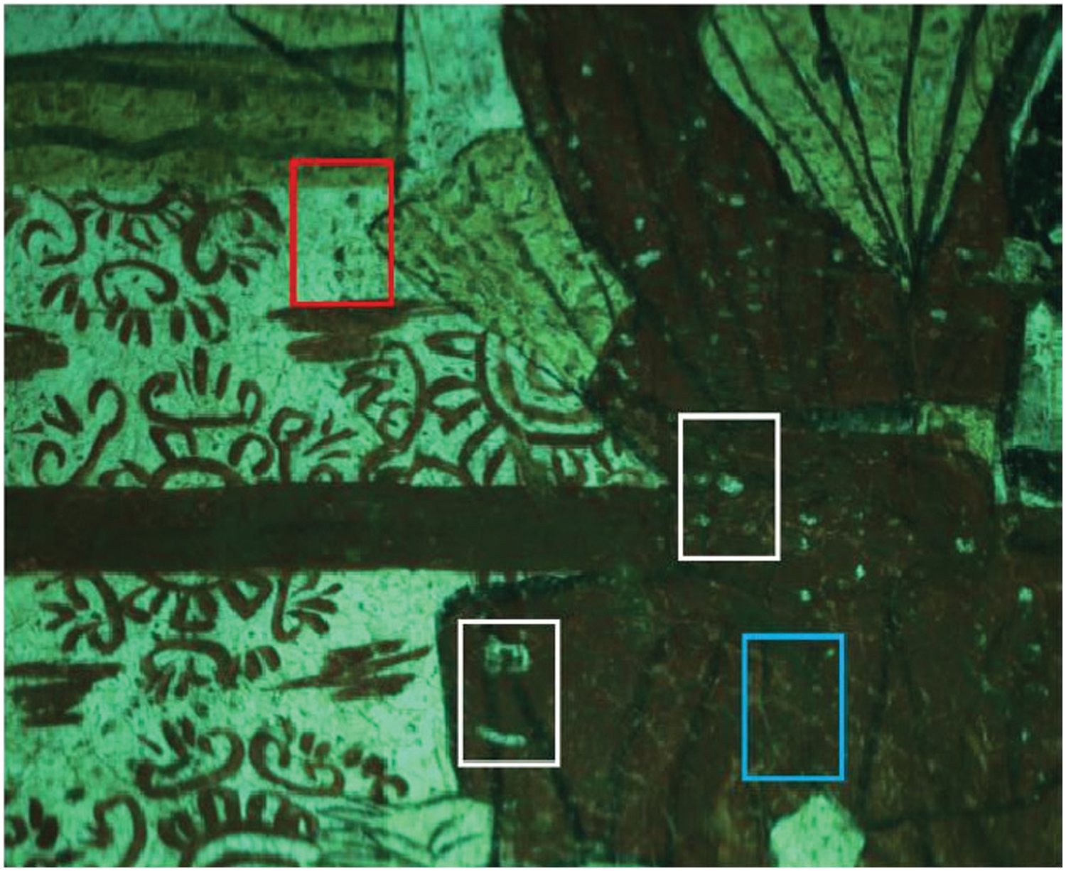
Figure 1: Types of mural damage: peeling (white frame), cracking (sky blue frame), and black spots (red frame)

There are two main categories of methods used for mural-based anomalous region detection: traditional machine learning methods, which can be broadly categorized into statistical methods, representational models, and tensor decomposition [1]. Statistical methods usually assume that the background adheres to a particular distribution, such as a multivariate Gaussian distribution, and then use Mahalanobis distance or Euclidean distance to recognize anomalous objects differing from the background distribution [2]. Among such methods, the RX (Reed-Xiaoli) detector is well known. It takes the original image as a background, assumes it follows a Gaussian distribution, and uses this to identify anomalous pixel points [3]. The Local RX (LRX) algorithm is an improved method, which uses a specific neighborhood of the pixel to be tested as a background and estimates the likelihood that the target pixel is an anomaly [4,5]. He et al. proposed a modified RX approach that incorporates extended multi-attribute profiles through an iterative process since most RX-type methods focus excessively on spectral information and ignore spatial information [6]. Representation model-based methods can perform anomaly detection without assuming the background distribution. Li et al. applied a combined sparse representation model of the background to recognize hyperspectral anomalies, working under the premise of a binary assumption [7]. The spatial and spectral features of hyperspectral images are highly correlated, causing the background distribution to exhibit global low-rank features, which allows the anomaly target to be localized with low-rank representation [8]. Tensor decomposition-based methods: Hyperspectral images can be considered as a third-order tensor cube, allowing better mining of spectral and spatial properties using tensor decomposition. Qu et al. performed anomaly detection using spectral unmixing [9,10]. Ma et al. proposed a hyper-Laplace regularized low-rank tensor decomposition method combined with a dimensionality reduction framework, accounting for both spatial and spectral information [11]. Li et al. proposed a Prior-based Tensor Approximation (PTA) method that combines the advantages of low-rank, sparsity, and smoothing in the tensor representation of hyperspectral images [12]. These traditional algorithms are widely used, have low operating environment requirements, and do not rely on a large number of training samples. However, due to the unevenness and variety of features in the damaged areas of mural images, these traditional methods can usually only recognize certain types of damage, such as single crack shapes and lacquer peeling. As a result, no single method can identify all abnormal areas on diverse mural surfaces. These methods lack uniformity, require significant labor costs, have low automation, and yield poor results.

The second category is deep learning-based methods. Traditional feature-based methods struggle to adaptively extract features according to the characteristics of the data, a problem that deep learning methods have effectively addressed. Deep learning-based anomaly detection methods are mainly classified into two categories: methods based on Autoencoders (AE) and methods based on Generative Adversarial Networks (GAN). Zhao et al. developed a spectral-spatial stacking self-encoder (LRaSMD-SSSAE) to extract deep features in the hidden space [13]. To reduce the dimensionality of the data and eliminate degraded spectral channels, Xie et al. proposed a spectral adversarial autoencoder (SC-AAE), which optimizes the model using adaptive weights and spectral angular distances [14]. Fan et al. designed Robust Graph Autoencoders (RGAE), based on the structure of the autoencoder, which substantially improved anomaly detection performance [15]. Based on the Generative Adversarial Network, Arisoy et al. proposed an unsupervised anomaly detection method for hyperspectral images [16]. Jiang et al. proposed a discriminative semi-supervised Generative Adversarial Network with a dual RX structure [17]. Cheng et al. proposed a novel Deep Feature Aggregation Network (DFAN) using an adaptive aggregation model, which combines an orthogonal spectral attention module with a background-anomaly category statistics module, and designed a novel multiple aggregation separation loss [18]. Lian et al. proposed a novel gated transformer network (GT-HAD) for hyperspectral anomaly detection, introducing an adaptive gating unit that can effectively differentiate between backgrounds and anomalies [19]. In deep learning anomaly detection, aside from the two main categories mentioned above, there are also image classification-based anomaly detection algorithms. These techniques differentiate between normal and anomalous data in a given feature space by training classifiers, mostly with supervised learning [20]. For example, Li et al. explored the effectiveness of transfer learning techniques for hyperspectral anomaly detection in a supervised manner [21]. Zhang et al. proposed an unsupervised Convolutional Neural Network model for extracting deep features from dictionary tensors [22]. Qiu et al. proposed a U-Net based extraction and analysis algorithm that can be used for anomaly detection of artifacts [23]. To improve the efficiency of background modeling, Zhang et al. also proposed a Hyperspectral Anomaly Detection method based on Attention-aware Spectral Difference Representation (HAD-ASDR) [24].

Mural paintings are difficult to access and require approval from the cultural protection department, which leads to less anomaly detection work on murals, with most research based on RGB images. Although RGB images conform to human visual perception, they contain only three bands of information, which is insufficient for comprehensive analysis of anomalous areas in murals. RGB images primarily rely on underlying features such as color and texture for anomaly detection. However, in mural images, different types of anomalies may exhibit similar underlying features. For example, black pigment in the mural and black spots caused by erosion may have similar color and texture features. This similarity makes detection prone to misjudgment and omission. Additionally, since the surface of the mural has many tiny cracks and slight color changes, the information in a standard RGB image may not be sufficient to reflect these subtle material changes, thus affecting detection effectiveness.

Through the above analysis, algorithms based on deep learning have become the mainstream in current mural painting anomaly detection work and have achieved certain results. The current problems faced by anomaly detection of murals using artificial intelligence are:

1) The difficulty of acquiring murals and the limited information provided by RGB images affect the detection results;

2) Murals contain a large number of anomalies with irregular and unbalanced distribution, and existing models lack the ability for complete contextual analysis, leading to suboptimal detection results with small samples;

3) Traditional convolutional neural networks suffer from feature redundancy and irrelevant feature interference, resulting in insufficient detection accuracy in complex backgrounds or noisy situations.

Based on the advantages of hyperspectral images, we propose a mural anomaly detection algorithm based on a hyperspectral multi-scale residual attention network (HM-MRANet). The major contributions of this paper are as follows:

1) Establishing a mural hyperspectral dataset to address the insufficiency of information in traditional RGB images for mural anomaly detection and to provide robust data support for detecting anomalous regions.

2) Proposing multi-scale residual spectral and spatial feature extraction modules to better capture multi-scale information, improve the network’s contextual analysis capability, and mitigate the impact of small sample data on detection.

3) Proposing the Enhanced Residual Attention Module (ERAM) to address the feature redundancy problem by simultaneously utilizing channel and spatial attention mechanisms, thereby enhancing the feature discrimination ability of the network and improving abnormal region detection accuracy.

2  Methods

A hyperspectral image contains hundreds of consecutive bands of spectral information, with each band reflecting different spectral characteristics. It has higher dimensions and a larger amount of data, providing richer spectral information than ordinary images. Fig. 2 shows a hyperspectral image of a mural, with three selected pixel points and their corresponding spectral characteristic curves displayed in Fig. 2a–c. Fig. 2a,c shows the spectral characteristic curves corresponding to pixel points in abnormal regions. Fig. 2a corresponds to black spots in the mural image, and Fig. 2c corresponds to pixel points where the material on the surface of the mural is abnormally detached. Fig. 2b shows the spectral characteristic curve of normal pixel points, which appear similar in color to those in Fig. 2a in the RGB image. However, their spectral characteristic curves show very clear differences. Therefore, hyperspectral images allow us to obtain information that is difficult to acquire from ordinary RGB images. By using hyperspectral imaging technology for anomaly detection in murals, we can extract spectral information to classify pixels with different materials and varying degrees of aging, thereby improving anomaly detection effectiveness. Moreover, due to the large number of anomalous points and their scattered and uneven distribution in mural images, it is more suitable to detect anomalous areas using the image classification method.

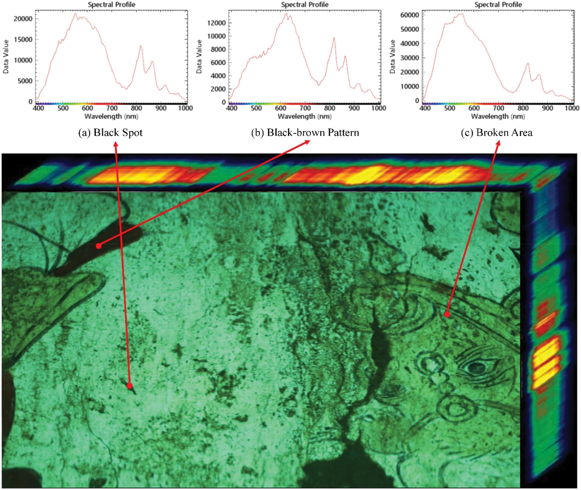
Figure 2: Examples of spectral curves for different types of pixel points in a mural hyperspectral image

In recent years, many classification networks based on hyperspectral images have been proposed and have achieved excellent results. The main one is the CNN (Convolutional Neural Networks) with three typical convolutional kernels. 1D CNN can only extract spectral curve information in one dimension, and 2D CNN can only extract spatial feature information in two dimensions. For complex mural images, relying solely on spatial or spectral information alone is insufficient for accurate pixel classification. However, 3D CNN can simultaneously extract spatial-spectral features in mural hyperspectral images, making it suitable for anomaly detection tasks.

Hu et al. introduced convolutional neural networks into hyperspectral image classification, but only used spectral information for classification [25]. Chen et al. proposed a 3D-CNN-based deep feature extraction method, utilizing both spatial and spectral information for classification [26]. Zhong et al. proposed a deep residual network model with joint spatial and spectral features (SSRN), which utilizes successive residual modules to learn spectral and spatial features separately, effectively improving classification accuracy compared to the above methods [27]. Wei et al. designed a Residual Dense Network model (ResDenNet) by combining residual and dense networks, which fully utilize discriminative features and improve the stability of the classification method [28]. Ravikumar et al. proposed a Deep Capsule Network (Deep Matrix Capsules) with an Expectation Maximization (EM) routing algorithm, specifically designed to adapt to nuances in the image, achieving good classification results [29]. Li et al. proposed a Central Vector Oriented Self-Similarity Network (CVSSN), based on two similarity metrics, to achieve efficient spatial-spectral feature learning [30]. Li et al. developed a model for Deep Cross-Domain Few-Shot Learning in hyperspectral image classification (DCFSL), employing the generative adversarial network approach for its design and training [31]. Zhang et al. proposed a Graph Information Aggregation Cross-Domain Few-Shot Learning method to improve image classification results through graph information aggregation [32]. Qiu et al. proposed an Extraction Algorithm Based on Multilayer Depth Features for Hyperspectral Images, which establishes a multilayer feature extraction framework and optimizes the classification effect [33]. Zhao et al. proposed a method based on Grouped Separable Convolutional Visual Transformer Network (GSC-ViT) for hyperspectral image classification, effectively capturing local spectral information by designing a Grouped Separable Convolution (GSC) module, achieving strong classification performance with relatively few training samples [34]. Ma et al. proposed a method based on Multi-Domain Few-Shot Learning (MDFL) to improve image classification [35]. Jiang et al. proposed a new graph-generated structure-aware transformer (GraphGST) that captures local-to-global correlations [36]. Chen et al. proposed an unsupervised multivariate feature fusion network (M3FuNet), using multiscale supervector correction (MSMC) and multiscale stochastic convolutional discretization (MRCD) as the spectral and spatial feature extraction methods. The obtained spectral-spatial joint features have high feature retention and strong spectral-spatial dependence, achieving very competitive results in hyperspectral image (HSI) classification [37].

Although 3D CNN has some advantages in image classification, it still faces several problems in anomaly detection of hyperspectral images:

1) Ordinary 3D CNN lacks multi-scale feature extraction, limiting its ability to fully explore effective spatial and spectral information and preventing effective feature fusion.

2) The large number of bands in hyperspectral images requires significant computational resources for anomaly detection using 3D CNN, and 3D CNN loses accuracy when learning from small sample data.

3) The high correlation and redundancy between the bands of hyperspectral images lead to serious overfitting problems during processing.

2.1 Network Infrastructure

To achieve anomalous region detection of murals, we use hyperspectral imaging to obtain mural information and conduct research based on 3D CNN. To solve the above problems of 3D CNN in anomaly detection, we propose an improved 3D CNN model that introduces spatial and spectral residual connectivity. We propose a multi-scale spectral and spatial feature extraction module to further capture multi-scale information. For feature fusion, we propose an enhanced residual attention module that uses the attention mechanism to select features more efficiently. To extract multi-scale features, we enhance the original pooling method by incorporating a spatial pyramid pooling module.

Between the spectral and spatial feature learning modules, we use Group Normalization (GN) [38] to replace the traditional Batch Normalization (BN) layer. Fig. 3 shows the overall flowchart of the HM-MRANet in this paper, which is structured as follows:

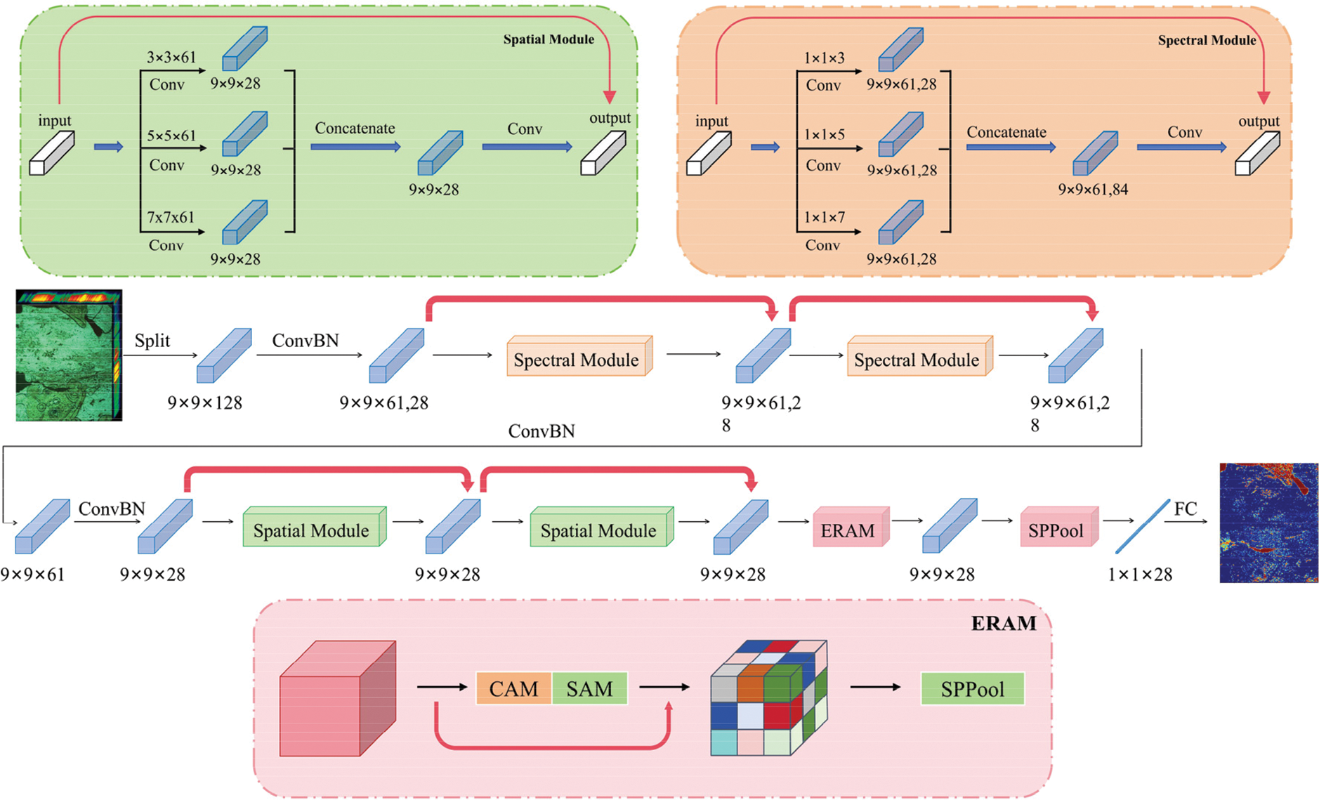
Figure 3: Overall flowchart of the network

1) Multi-scale residual spatial-spectral feature extraction module, including spectral feature learning module (Spectral Module) and spatial feature learning module (Spatial Module). In the network, we use two Spectral Modules and two Spatial Modules, with each module containing two convolutional layers and BN layers in loops for feature extraction. Each module contains residual structures, shown by the red arrows in the figure, for skip connections to stabilize the training process and accelerate convergence. We propose a multi-scale convolutional approach, using three convolutional kernels of different sizes in each module to acquire different scales of spectral features of the input image, thereby enhancing feature extraction capability.

2) Enhanced Residual Attention Module (ERAM), using both channel attention and spatial attention mechanisms to adaptively assign attention weights to the feature map.

3) The Spatial Pyramid Pooling (SPP) module [39] and the fully connected layer, performing multi-scale feature aggregation and classification outputs, and finally obtaining a probability map corresponding to each pixel point, with values ranging from 0 to 1.

CNN models face a problem where classification accuracy decreases as the number of convolutional layers increases. This accuracy degradation can be mitigated by constructing residual modules between layers. We propose spectral and spatial residual modules to address the issue of accuracy degradation resulting from the increased number of convolutional layers. This work includes three main feature extraction modules: the spectral feature extraction module, the spatial feature extraction module, and the enhanced residual attention module. All these modules include consecutive 3D convolutional layers sliding in spectral and spatial dimensions for convolutional operations, with padding to ensure constant input and output dimensions, facilitating the implementation of residual connections.

After preprocessing the original image, the hyperspectral image data inputted into the network has dimensions of 9 × 9 × 128 (where the 3D neighborhood of each pixel is considered, with the center pixel’s category serving as the label), and the original data contains both rich and redundant spectral information. To eliminate this redundancy, we employed 28 convolutional kernels of size 1 × 1 × 7 to perform convolutional operations, aiming to reduce spectral dimensionality and data redundancy. Following the convolution operation, 28 feature cubes of size 9 × 9 × 61 were generated. Subsequently, two consecutive spectral residual blocks, each containing four convolutional layers and two constant mappings, were added. In these blocks, all convolutional layers were padded to preserve the structure of the output feature cubes. Finally, a convolution kernel of size 1 × 1 × 61 was used to maintain the spectral features, followed by another dimensionality reduction operation to compress the data from 61 dimensions to 28 dimensions, ensuring it is suitable for input into the spatial feature learning stage.

In the spatial feature learning section, the structure is similar to that of the spectral feature learning section, differing only in the size and structure of the data. Again, two spatial residual modules are used. At the end of the two feature learning sections, the extracted spectral-spatial feature volume of 9 × 9 × 28 is converted to a one-dimensional feature vector using a spatial pyramid pooling layer to generate the output values using a fully connected layer.

In the spectral and spatial feature learning module, we use two consecutive spectral and spatial residual modules, and this design has the following three advantages over using only one residual module: (1) Enhancing feature extraction ability: The main purpose of the spectral and spatial modules is to extract useful features from the data. Two consecutive feature extractions, compared to a single module, allow for deeper extraction, resulting in more refined and enhanced features. (2) Improving model robustness: Using two modules consecutively makes it easier for the model to capture stable features, suppress noise, and reduce information loss during feature extraction. (3) Promoting feature fusion and interaction: Consecutive use of modules promotes the fusion and interaction between different features, making the model more effective in integrating spectral and spatial information. This approach allows the model to better understand and utilize the integrated features in the data, thereby improving overall classification or detection performance.

Due to the large amount of data in hyperspectral images, model training often requires smaller batch sizes compared to general image data. However, under conditions of small batch sizes, the instability of batch normalization can easily lead to poor model training, whereas group normalization can provide more stable normalization by grouping feature channels and normalizing within each group.

Secondly, the spatial and spectral features of hyperspectral data exhibit significant differences across various scales, and the feature distributions during the learning process of spectral and spatial features follow distinct statistical laws. Group normalization can better capture and fuse these features. After comparing the experimental results, it was found that using group normalization between the two modules resulted in a noticeable improvement compared to using batch normalization. However, the benefits of group normalization in other areas were less pronounced. Therefore, we ultimately chose to use the GN layer between the spectral and spatial feature learning modules instead of the traditional BN layer for normalization.

After completing the extraction of spectral and spatial features, we set up an Enhanced Residual Attention Module before the Pooling and Fully Connected Layers to strengthen the effect of residual connectivity and introduce the attention mechanism before data output. This architecture enables gradients in the higher layers to propagate back to the lower layers quickly, facilitating and standardizing the model training process. In contrast to standard 3D CNN, the network mitigates accuracy degradation by adding skip connections between each partitioned layer, formulating the hierarchical feature representation layer as a continuous module of residuals.

2.2 Multi-Scale Residual Spatial-Spectral Feature Extraction Module

2.2.1 Residual Link

Deepening the layers of a deep learning network can improve its learning and feature expression abilities, but experiments have shown that beyond a certain depth, increasing the number of layers does not improve performance and can cause network degradation. As the number of layers increases, accuracy will saturate or even decline. To solve the problem of network degradation, He et al. proposed the method of residual learning [40]. As shown in Fig. 4, the network input is x, the desired feature mapping is H(x), and after adding the residual connection, the original mapping is denoted as F(x) + x. In the process of forward propagation, residual learning can realize constant feature mapping, thus avoiding network degradation while increasing the number of layers.

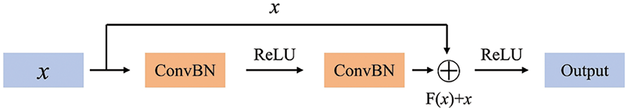
Figure 4: Flowchart of the residual learning module

The residual connection is realized by the following equation:

y=F(x,{Wi})+x(1)

2.2.2 Spectral Feature Extraction Module

Fig. 5 shows the multi-scale residual spatial-spectral feature extraction module of this paper, which uses the above residual units in both the spectral and spatial feature extraction modules. It is designed to solve the problem of gradient vanishing during the training process of deep networks.

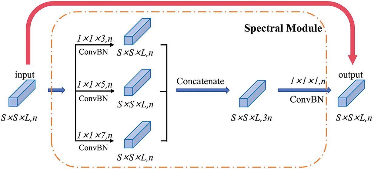
Figure 5: Flowchart of the spectral feature extraction module

Batch Normalization is applied after each convolutional layer using the following formula:

x^(k)=x(k)−µBσB2+∈(2)

Due to the wide range of bands, high spectral resolution, and strong spatial correlation of hyperspectral images, this paper designs a multi-scale feature extraction module for both spectral and spatial dimensions, adding a branching structure to the residual module. In each branch structure, different sizes of convolution kernels are used to obtain different scales of features in the input image. The output feature maps are then connected using the splicing operation, and the channels are downscaled by a 1 × 1 × 1 convolution to achieve fusion with the shallow features. We incorporate a batch normalization layer and a ReLU activation following each convolutional layer.

In the first convolution operation shown in Fig. 5, three different sizes of convolution kernels are used for feature extraction: 1 × 1 × 3, 1 × 1 × 5, and 1 × 1 × 7. By adjusting their step sizes and edge padding to ensure that the outputs have the same data size, when inputting S × S × L sized data with a batch size of n, a batch size of 3n is obtained after the convolution operation with three convolution kernels. Let the input data be xi, and the output data be xi+2, then there are:

xi+2=xi+H{T[F1(xi), F2(xi), F3(xi)]}(3)

Fs(xi) (s = 1, 2, 3) in this equation denotes the nonlinear operation of the convolution kernel with different spectral dimension sizes, T(•) denotes splicing the output data of the convolution layer, and H(•) denotes the dimensionality reduction operation on the channel.

The spectral residual module and the spatial residual module contain two convolution operations. The first is a multiscale convolution operation that sets the intermediate process data to xi+1. The two convolution operations are used in the successive filter banks of the ith and (i+1)th layers, respectively. The spatial dimensions of the three-dimensional feature cubes xi+1 and xi+2 are kept constant at S × S × L by a specific padding strategy, and the residuals are constructed. The spectral residual architecture can be expressed as follows:

xi+2=xi+F(xi; θ)(4)

F(xi; θ)=R(x^i+1)∗hi+2+bi+2(5)

x=R(x^i)∗hi+1+bi+1(6)

where θ = {hi+1, hi+2, bi+1, bi+2}, xi+1 denotes the input three-dimensional feature cube in layer i+1, and hi+1 and bi+1, denote the spectral convolutional kernel and bias in layer i+1, respectively. In fact, the convolution kernels hi+1 and bi+1 are composed of one-dimensional vectors and can be viewed as special cases of three-dimensional convolution kernels. The output tensor of the spectral residual module also consists of n three-dimensional feature cubes.

2.2.3 Spatial Feature Extraction Module

As shown in Fig. 6, three convolution kernels of different sizes are also used for feature extraction in the spatial residual module, for hyperspectral data with input size W × W × L, a convolution kernel of size r × r × 61 (r = 3, 5, 7) is used for the unit with input xj and output Xj+2, respectively, which gives:

xj+2=xj+H{T[D1(xj), D2(xj), D3(xj)]}(7)

where Ds(xj) (s = 1, 2, 3) denotes the nonlinear operation of the convolution kernel with different spatial dimensions.

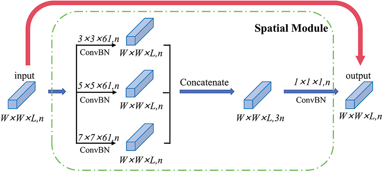
Figure 6: Flowchart of the spatial feature extraction module

In the spatial module, the focus is mainly on the continuous filter banks Hq+1 and Hq+2, and spatial feature extraction is performed using 3D convolution kernels of different sizes, which have a spectral depth d equal to the depth of the spectrum of the input 3D feature cube xq. The spatial sizes of the feature cubes xq+1 and xq+2 are kept constant at W × W × L.

The spatial residual architecture can be expressed as follows:

xq+2=xq+D(xq; ξ)(8)

D(xq; ξ)=R(x^q+1)∗Hq+2+bq+2(9)

x=R(x^q)∗Hq+1+bq+1(10)

where ξ = {Hq+1, Hq+2, bq+1, bq+2}, xq+1 denotes the three-dimensional input feature volume in layer q + 1, and Hq+1 and bq+1 denote the spatial convolution kernel and the deviation in layer q + 1, respectively. In contrast to the spectral residual module, the convolution filter bank in the spatial residual module contains the 3D tensor, and the output of this module is the 3D feature volume.

2.3 Enhanced Residual Attention Module (ERAM)

The traditional residual module is realized by skip connections, which effectively mitigates problems such as gradient vanishing and gradient explosion in deep networks but does not account for the importance differences between different channels. Based on this, this paper proposes an enhanced residual attention module for adaptive feature extraction, as shown in Fig. 7. Building on the traditional residual module, channel attention and spatial attention mechanisms are introduced, and different weights are assigned to each spectral and spatial channel. This improves the model’s performance and representation ability in the following aspects:

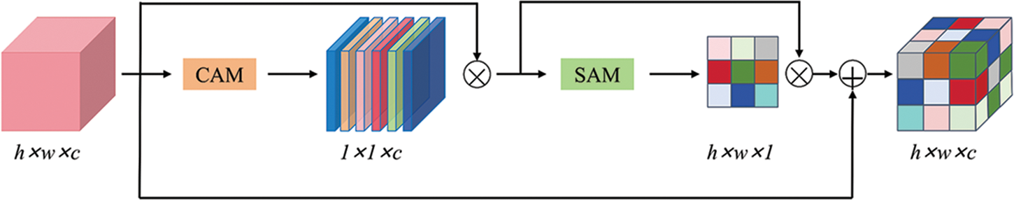
Figure 7: Flowchart of the enhanced residual attention module

1) Enhancing feature representation: Adaptively adjusting the weights of each channel through the CBAM attention module allows the model to better focus on important features. This is especially important for outlier detection in hyperspectral images, which usually have high dimensionality and complex feature distribution.

2) Better feature reuse: The residual module combined with the attention module enables better reuse of features, which enhances the model’s generalization capacity and stability. The residual module mitigates the gradient vanishing problem in deep networks through skip connections, while the attention module further enhances the flexibility of feature representation.

3) Enhancing the network’s selection ability: The module enhances the network’s selection ability by introducing an attention mechanism that enables the network to dynamically adjust the feature importance of each channel. This is a significant advantage for outlier detection in mural hyperspectral images, which usually requires precise discrimination between important features and background noise.

In this paper, we improve the design of residual attention module based on Convolutional Block Attention Module (CBAM) [41]. CBAM is a lightweight architecture, based on which we integrate the residual connection as shown in Fig. 7, the channel attention module CAM, and the spatial attention module SAM, defining their operations as AS(•) and AC(•), respectively, given an intermediate feature map fx, we obtain the attention weight Matten as:

Matten=As(Ac(fx)⊗fx)(11)

where ⊗ denotes the element-by-element multiplication. Next, the attention weights are multiplied with the original input features and then jump residual joining is performed so that a weighted feature map fatten can be obtained, which assigns different weights to each channel and region, thus favoring more important features and ignoring some minor features. This attention mechanism module improves the network’s ability to learn important features by adaptively learning and assigning attention weights, which helps to improve the classification results.

fatten=fx+Mattne⊗fx(12)

2.3.1 Channel Attention Module

The channel attention module CAM focuses on assigning adaptive weights to different feature channels, and assigns different importance to each spectral dimension in the mural hyperspectral image anomalous region detection task. As shown in Fig. 8, given the input feature map fh × w × c, the first step is to compress the features through the average pooling layer and the maximum pooling layer, respectively, to obtain the average pooling feature AP(f) and the maximum pooling feature MP(f).

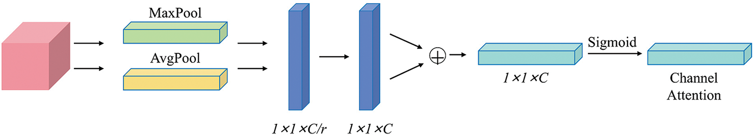
Figure 8: Flowchart of the channel attention module

Then, these two obtained features are transmitted to the shared network, defined as F(•), for capturing the internal relationship between the feature channels. Finally, the channel attention vector Ac(f) = (0, 1)1×C, defined as σ(•), is obtained by the sigmoid operation, denoted as:

Ac(f)=σ(F(AP(f))+F(MP(f)))(13)

2.3.2 Spatial Attention Module

As shown in Fig. 9, the spatial attention module SAM is able to assign different adaptive weights to spatial feature regions, in which the two features generated by average pooling and maximum pooling are jointly connected to a common convolutional layer, which is utilized to explore spatial relationships in the data. The spatial attention graph can be represented as follows:

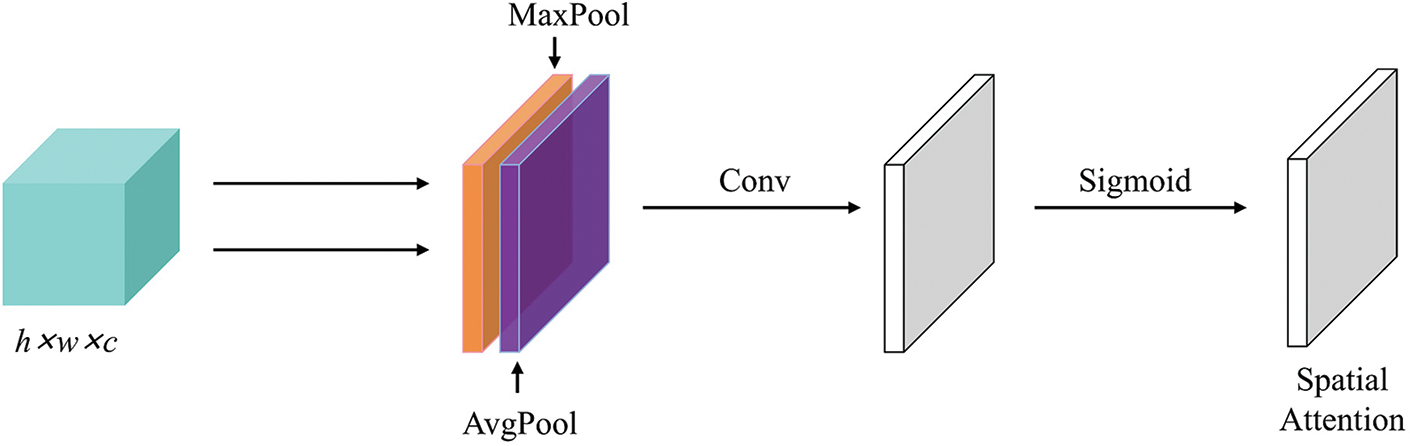
Figure 9: Flowchart of the spatial attention module

As(f)=σ(Conv([AP(f); MP(f)]))(14)

2.4 Spatial Pyramid Pooling Module

The basic principle of the Spatial Pyramid Pooling (SPP) module is to generate a fixed-size feature representation by capturing different scale features of an image through multi-scale pooling operations. This approach allows the network to accept inputs of arbitrary size without cropping or scaling the input image. The SPP module performs multi-scale pooling operations on the input feature maps and then joins the pooled feature maps to form a fixed-length feature vector.

By performing pooling operations at multiple scales, the SPP module can capture feature information at different scales, allowing the network to process input images of arbitrary size without cropping or scaling the input images. Through multi-scale pooling operations, the SPP module can improve the robustness of feature representation, enabling the network to perform better when facing inputs of different scales. Compared to the fully connected layer, the SPP module reduces computation and improves performance in the feature extraction stage. In this model, the SPP module is applied at the end of feature extraction to replace the pooling layer of the 3D CNN, converting the feature maps of hyperspectral images into fixed-size feature vectors. The specific operation flow is as follows:

1) Feature extraction: The features of the hyperspectral image are extracted by the null spectrum feature extraction module and the enhanced residual attention module to generate the feature map.

2) Multi-scale pooling operation: 1 × 1, 2 × 2, and 4 × 4 pooling scales are used in this model, and the pooling operation of each scale generates corresponding feature vectors.

3) Feature connection and classification: The feature vectors pooled at different scales are connected to form a fixed-length feature vector. Finally, the fixed-length feature vector output from the SPP module is passed to the fully connected layer to complete the final anomaly detection task.

As shown in Fig. 10, the sizes of the SPP module used in this experiment are [1, 2, 4]. After three different pooling operations, the input feature map x is pooled into different sizes, and the output feature map is channel transformed by a 1 × 1 convolutional layer. Each pooled feature map is channel transformed by a 1 × 1 convolutional layer to ensure that the size of the output feature map remains unchanged. Each convolved feature map is then interpolated to the size of the original input feature map, and all the interpolated multi-scale feature maps are spliced together in the channel dimensions to form the final output feature maps, which are then passed to the fully connected layer. In this way, the diversity and robustness of feature extraction are enhanced, making it suitable for hyperspectral mural images with various anomalies and different sizes and patterns.

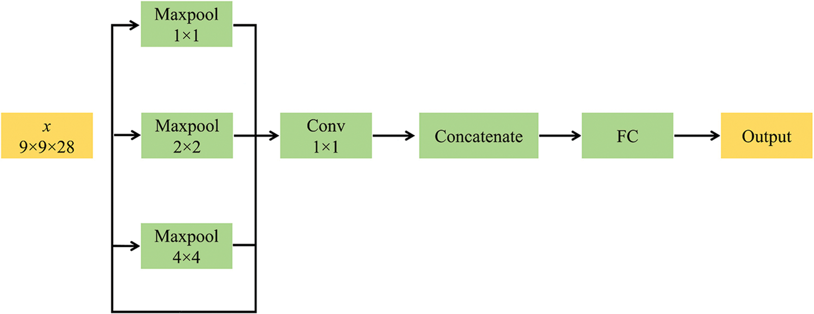
Figure 10: Flowchart of the SPP module

3  Experiments

3.1 Datasets and Evaluation Indicators

The datasets used in this experiment are all derived from mural data collected on-site by the self-developed hyperspectral imaging instrument, as shown in Fig. 11, where the spectrometer adopts the push-scanning imaging method for data acquisition. There are 50 hyperspectral images in this dataset, in .raw format. Each hyperspectral image is 1392 × 1705 pixels, containing 128 channels. The acquired hyperspectral data are manually labeled by professionals, classifying all pixel points in the images into two categories: anomalies and background points. The labeled data were randomly divided into training, testing, and validation sets with proportions of 70%, 20%, and 10%, respectively. Out of a total of 50 images, 35 images were allocated to the training set, 10 images to the testing set, and 5 images to the validation set. These data provide relatively rich and accurate information for subsequent classification.

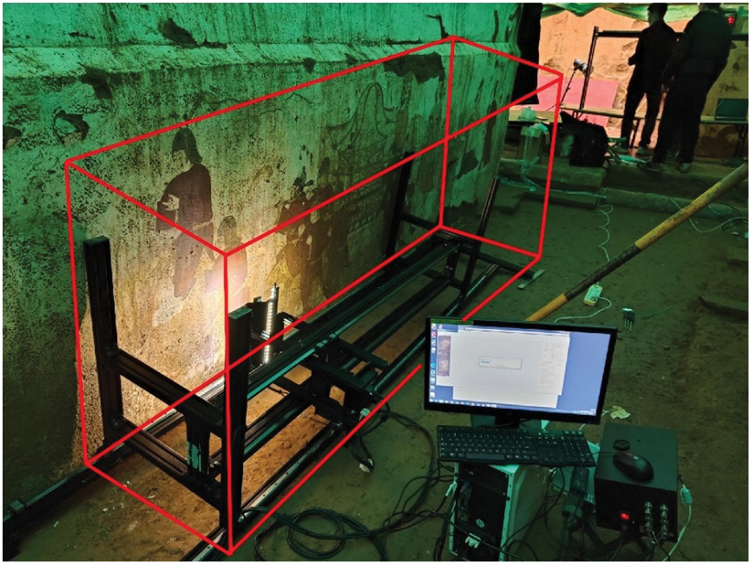
Figure 11: Mural hyperspectral image acquisition site, the equipment shown in the red area of the figure is the spectrometer, consisting of horizontal and vertical rails, support components, lighting components, cameras, etc.

In this paper, three evaluation metrics for anomaly detection, including ROC curve and AUC value, Specificity, and Accuracy, are used to evaluate the anomaly detection performance of the model. A visualization graph of the detection results is also included as an evaluation criterion.

1) Receiver Operating Characteristic (ROC) and Area Under Curve (AUC):

In this experiment, ROC and AUC are selected as quantitative metrics for measurement. Visualized detection results are provided to comprehensively assess the efficiency of anomaly detection in hyperspectral images.

The ROC curve is a graphical tool for evaluating the classification performance of binary classifiers, commonly used in threshold selection and decision analysis. It represents the results of multiple confusion matrices and demonstrates the performance of the model under different thresholds, enabling a comprehensive assessment of the model’s classification ability rather than just performance under a single threshold. It plots the True Positive Rate (TPR) and False Positive Rate (FPR) at different judgment threshold levels. The formula is calculated as:

TPR=TPTP+FN(15)

FPR=FPFP+TN(16)

True Positive (TP) refers to correctly identifying areas of an image that contain anomalies. False Positive (FP) occurs when the model incorrectly marks normal regions as anomalies. True Negative (TN) is when the model accurately recognizes normal regions as non-anomalous. Finally, False Negative (FN) happens when the model fails to detect an anomaly and incorrectly classifies it as a normal region.

The AUC value is an evaluation index calculated based on the ROC curve, taking a value from 0 to 1. The larger the AUC value, the more accurate the classification results. Conversely, the closer the AUC value is to 0.5, the less accurate the results, indicating the prediction is similar to a coin toss and has no reference value.

2) Specificity

Specificity, also known as the true negative rate, indicates the ability of the model to correctly recognize negative samples. Specificity is defined as follows:

Specificity=TNTN+FP(17)

Specificity indicates the proportion of negative samples that are correctly identified as negative.

3) Accuracy

Accuracy is the percentage of all samples that are correctly categorized. The accuracy rate is defined as follows:

Accuracy=TP+TNTP+TN+FP+FN(18)

4) Visualization of test results

In addition to the above quantitative metrics for qualitatively comparing the measurement algorithms, pseudo-color plots of the dataset, labeled anomaly reference plots, and color images representing the detection results of the various algorithms are included in this paper for visual comparative assessment of the effectiveness of the methods.

3.2 Results

3.2.1 Parameter Settings

All experiments were conducted in the PyTorch framework and run on NVIDIA GeForce RTX 3080 GPUs. We tested the number of convolutional kernels from 8 to 32 to determine the optimal configuration. BN, GN, and 50% dropout regularization methods were used to normalize the training process. The batch size was set to 50. During the training process, we used BCEWithLogitsLoss as the loss function and trained with the Adam optimizer, with a learning rate set to 0.001 for 30 iterations. The loss function is defined as follows:

BCE With Logits Loss=1N∑i=1N(yi⋅log⁡(σ(pi))+(1−yi)⋅log⁡(1−σ(pi)))(19)

where σ(x) is the Sigmoid function, log is the natural logarithm, pi denotes the probability that the sample is predicted to be a positive case, and yi is the true label of the sample, which in this experiment is 0 and 1, indicating whether the sample belongs to a positive or negative case.

3.2.2 Ablation Experiment

To verify the effectiveness of the anomaly detection algorithms proposed in this paper, we set up a series of ablation experiments for the multi-scale convolutional structures in the Spectral Feature Extraction module and Spatial Feature Extraction module, the Enhanced Residual Attention module, and the Spatial Pyramid Pooling module. The results of the ablation experiments are shown in Table 1.

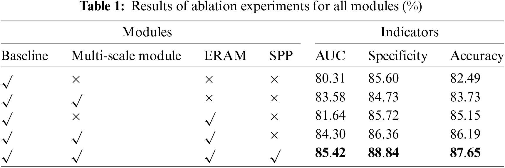
As seen in Table 1, after introducing multi-scale convolution, the AUC scores show a significant improvement, demonstrating that the multi-scale convolution operation module can effectively enhance the representation of the 3D CNN network and achieve more accurate detection. Although Specificity decreases by less than one percent, it still provides a significant overall improvement in the model’s effectiveness. Similarly, the introduction of the Enhanced Residual Attention module and the SPP module both increase the efficiency of our network in detecting anomalies in mural hyperspectral images.

3.2.3 Comparison Experiment

To demonstrate the effectiveness of the proposed method in this paper, we selected DCFSL [31], CVSSN [30], 3D CNN [26], Deep Matrix Capsules [29], and SSRN [27] as comparison networks, all of which are image classification networks that have shown good results on publicly available datasets. All methods use the same dataset, preprocessing method, hyperparameters, and loss functions for model training.

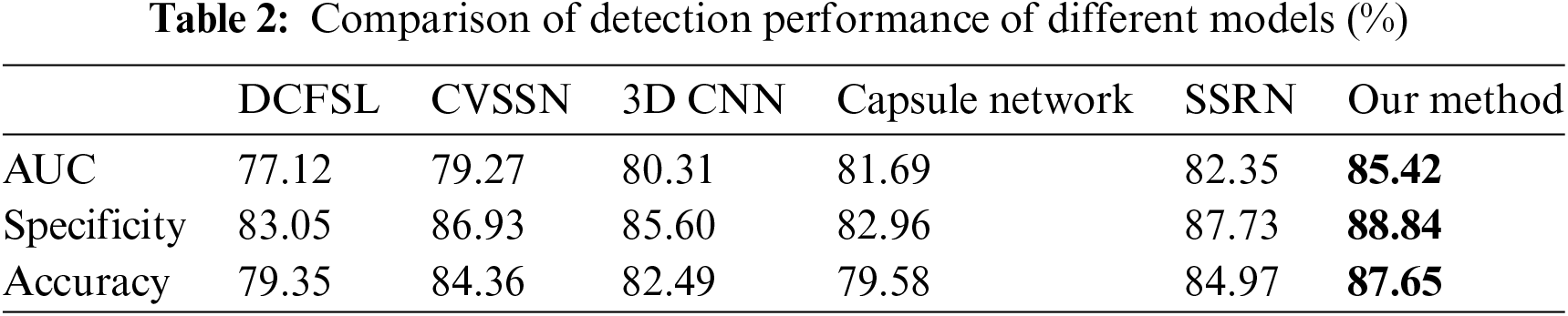
Table 2 shows the AUC value, Specificity, and Accuracy of our method compared to other methods. Our method achieved AUC, Specificity, and Accuracy values of 85.42%, 88.84%, and 87.65%, respectively. Compared to other methods, these evaluation indexes show a certain degree of enhancement, indicating the superiority of our method in detecting anomalies in hyperspectral images of murals.

To more intuitively represent the advantages of our model over other models, we selected four representative images and plotted their ROC curves and visualized prediction images. Fig. 12 shows the pseudo-color images of these four hyperspectral images. All four images are pseudo-color images of Tang tomb murals captured by the mural hyperspectral image acquisition system. Each image has different degrees and types of anomalous regions, as shown in the red box, to verify the effect of anomaly detection. In Fig. 12a, there is a large white shedding-like area in the upper right corner, which is a special type of anomaly. In Fig. 12b, there are cracks in the lower left corner, and the colors of the cracks are very close to the lines of the background image, making it difficult to distinguish whether it is an anomaly or a normal pattern in an ordinary RGB image. In Fig. 12c, there is a continuous piece of small black spots on the right side, and the colors are in different shades, but all of them are anomalous. In Fig. 12d, there is a relatively large black contaminated area in the upper right corner, which could be mistaken for the pattern in the mural, but can be distinguished using spectral information.

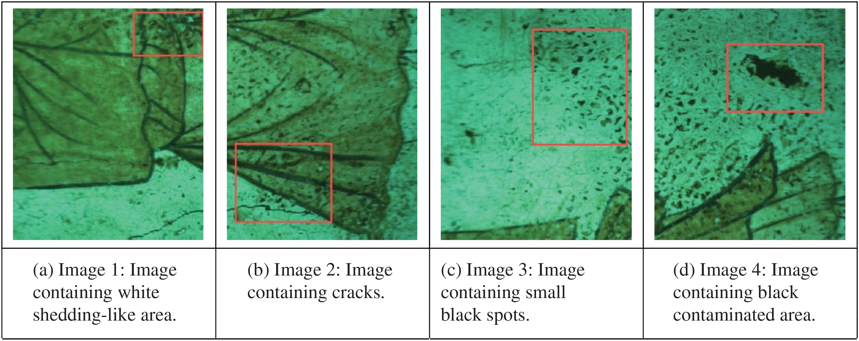
Figure 12: Four images of Tang tomb murals for display

Fig. 13 shows the ROC curves of the detection results of the six models on the anomalous regions of the four Tang tomb mural images mentioned above. The results indicate that the method proposed in this paper has the best performance in the detection task on all four images. Fig. 14 lists the visualized prediction maps of our method and each comparison method on the four mural images. The color of each pixel in the prediction map indicates its probability of being an anomaly: dark blue represents a probability of 0, and red represents a probability of 1. The closer the color is to red, the higher the probability that the network considers it an anomaly.

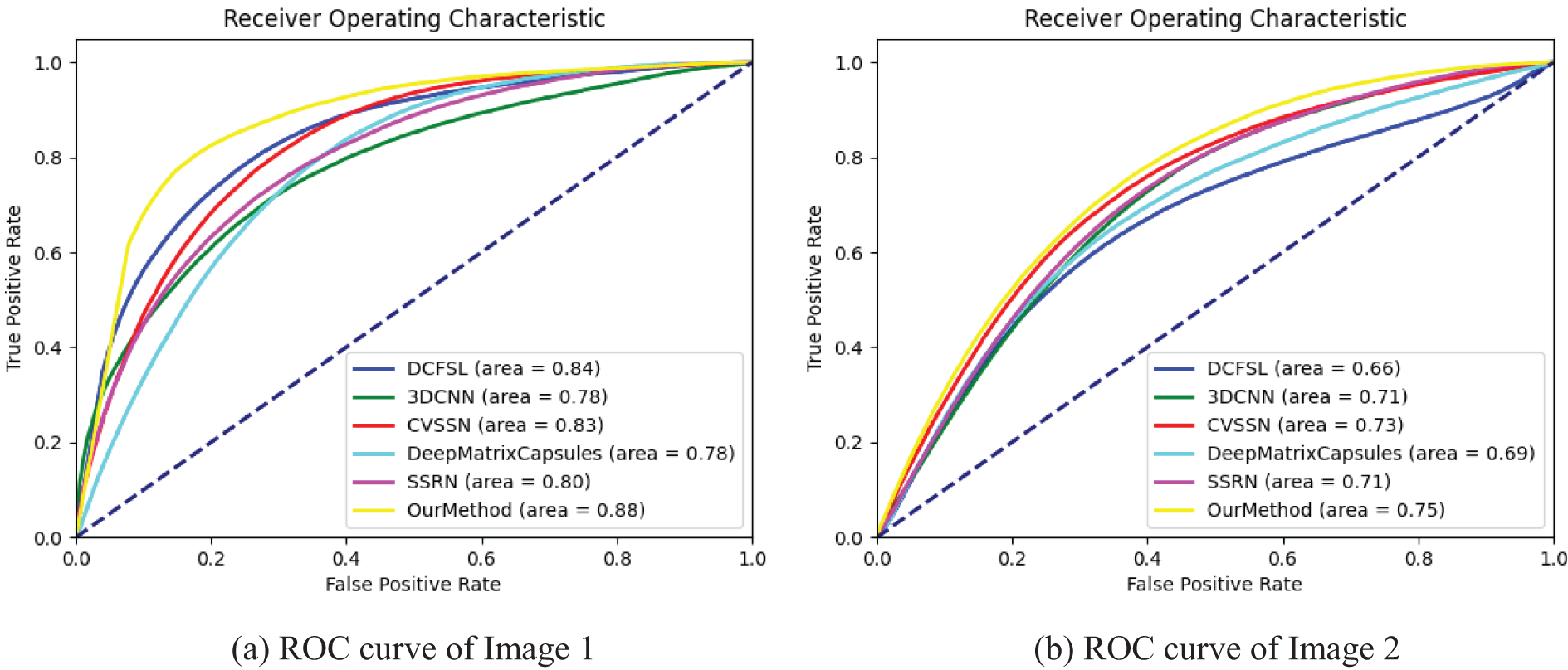
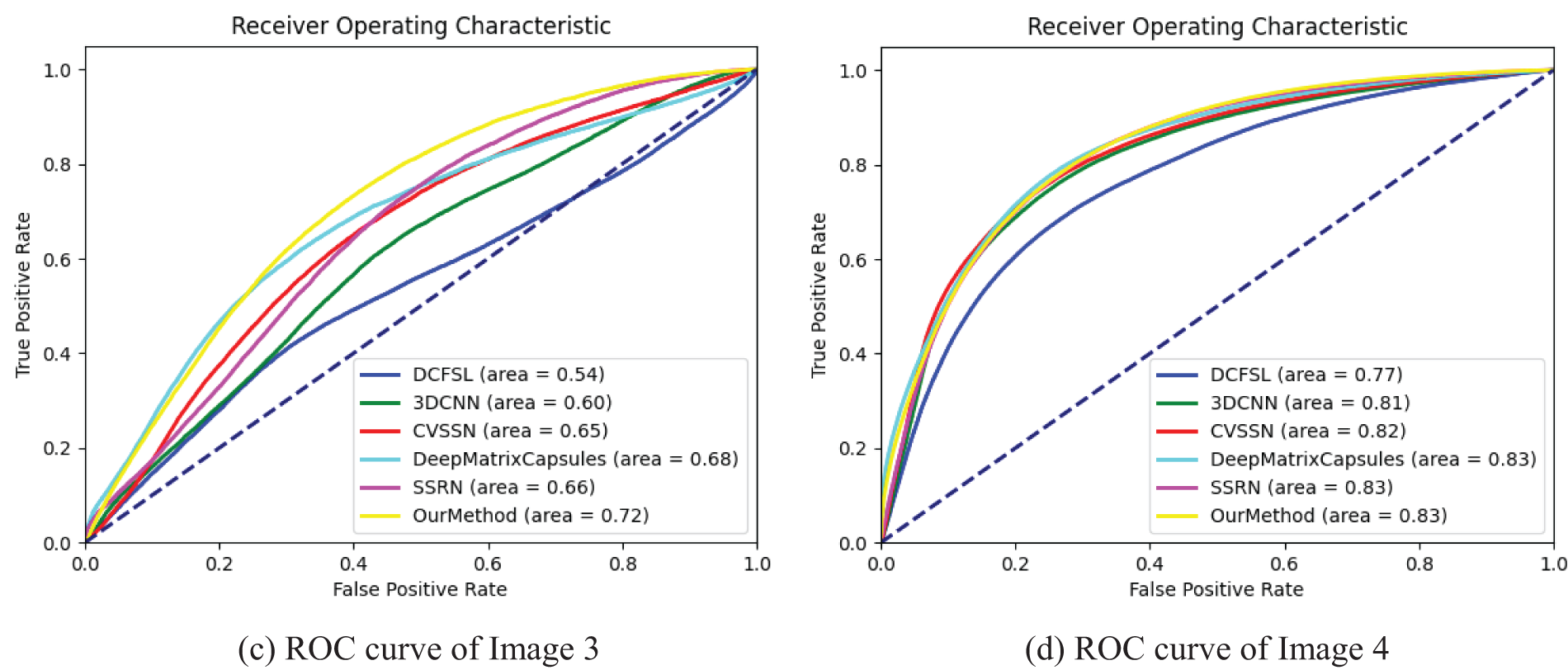
Figure 13: ROC curves of anomalous region detection results of six models on four Tang tomb mural images

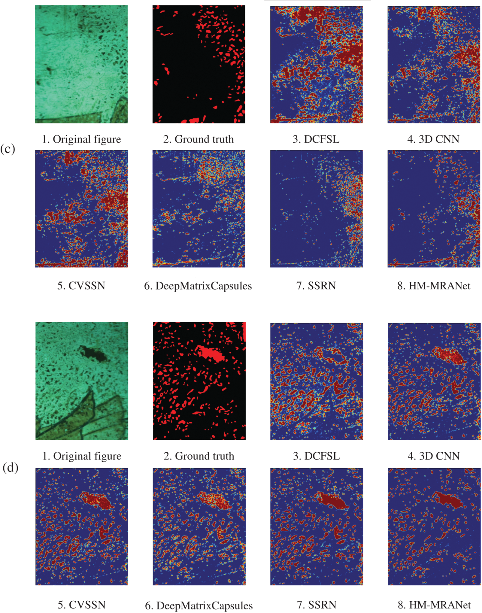
Figure 14: Visualization of anomalous region detection results of six models on four Tang tomb mural images. (a) The results of Image 1. (b) The results of Image 2. (c) The results of Image 3. (d) The results of Image 4

From the figure, it can be seen that all six models have some effect on the detection of anomalous regions of the mural, but their performance varies significantly. Among them, the DCFSL algorithm misidentifies the largest black spot area as a normal area in Fig. 14d, recognizes many normal line patterns as anomalies in Fig. 14a, and has more misdetections in the other two images, proving ineffective. 3D CNN, as a more classical image classification network, is able to detect most anomalies, but in each image, a certain number of false detections existed. CVSSN performed similarly, detecting more normal lines as anomalies. Deep Matrix Capsules had a more significant improvement compared to the previous networks, but many pixel points were detected close to the middle of the range and could not achieve good differentiation. SSRN’s detection was more desirable, but none of these contrasting models did a good job of detecting anomalies in the smaller anomalous regions.

The method in this paper achieves the best detection results compared to the labeled images. In Fig. 14a, our model achieves high accuracy compared to the other models, and there are few pixels with intermediate values in the result graph, indicating that the model’s discriminative performance is stronger than that of the comparison models. In Fig. 14b, the percentage of black thick line patterns classified as anomalous regions by our method is the least compared to other models. In Fig. 14c, although there is some degree of misdetection, such as misdetecting parts of the black thick lines as anomalies, it has good detection results for most regions. In Fig. 14d, SSRN and our model have the best detection effect on large black spots, but SSRN’s detection result has more probable pixel points with intermediate values, while our model has higher accuracy and is more stable.

Due to the introduction of a multi-scale spectral and spatial feature extraction module, the multi-scale information in mural hyperspectral images is captured effectively. Compared to single-scale or simplistic feature extraction methods used in other models, our multi-scale feature extraction module captures anomalous regions at various scales more comprehensively, particularly when addressing small and scattered anomalies, demonstrating a significant advantage and resulting in high recognition accuracy in the initial images. The incorporation of residual structures and attention modules allows the model to concentrate on key feature regions and enhances its discriminative ability, particularly in addressing the issue of false detections prevalent in other models when detecting small areas.

In summary, our model can effectively overcome the fragmented distribution of anomaly regions in mural hyperspectral images, has stronger feature extraction and discrimination ability compared with other models, and can maintain good detection results with a small number of samples, possessing stronger robustness than other models.

4  Conclusion

1) To address the limited information provided by ordinary RGB images for mural painting anomaly detection, we adopt hyperspectral imaging. We propose a mural anomaly detection algorithm based on a hyperspectral multi-scale residual attention network (HM-MRANet), construct a mural painting database, and carry out research on a hyperspectral dataset to leverage the information-rich advantage of hyperspectral data to improve anomaly region detection.

2) To address the small number of hyperspectral image samples and insufficient contextual expression ability of existing models, we propose a multiscale residual null spectrum feature extraction module to better capture multiscale information and improve feature extraction on small samples.

3) To address the widely distributed and cluttered anomalies in mural painting hyperspectral images, we propose the enhanced residual attention module and SPP pooling module. These modules enhance the network’s ability to learn global context information through channel and spatial dual-attention mechanisms, further improving feature extraction efficiency. The pooling module improves the characterization capability of the 3D CNN, enhancing the network’s performance in detecting anomalous regions in mural hyperspectral data with minimal increase in computational cost.

Experimental results show that our multi-scale residual feature extraction module and attention mechanism are of great importance in hyperspectral image restoration.

During the research, the following deficiencies were identified and need further study in the future:

1) The number of databases is limited. We will continue to construct richer datasets in the future to create conditions for detecting anomalous areas of murals using deep learning methods.

2) We will further optimize the network structure by reducing the number of layers and the size of convolutional kernels. We will also explore model compression techniques such as pruning and knowledge distillation, and consider advanced convolutional neural network architectures to develop a lighter network while enhancing its performance.

3) Since the research is currently conducted only on indoor murals, the network’s generalization ability needs to be verified and strengthened. Future research will adapt to a wider range of application scenarios and more complex environmental conditions, while exploring the potential of the model in multi-task learning and cross-modal learning, to better assist archaeologists in restoring mural paintings.

Acknowledgement: The authors also gratefully acknowledge the helpful comments and suggestions of the reviewers, which have improved the presentation.

Funding Statement: This work is supported by Key Research and Development Plan of Ministry of Science and Technology (No. 2023YFF0906200). Shaanxi Key Research and Development Plan (No. 2018ZDXM-SF-093) and Shaanxi Province Key Industrial Innovation Chain (Nos. S2022-YF-ZDCXL-ZDLGY-0093 and 2023-ZDLGY-45). Light of West China (No. XAB2022YN10). The China Postdoctoral Science Foundation (No. 2023M740760). Shaanxi Key Research and Development Plan (No. 2024SF-YBXM-678).

Author Contributions: Bolin Guo and Shi Qiu performed the experiments. Pengchang Zhang and Xingjia Tang analyzed the data. All authors reviewed the results and approved the final version of the manuscript.

Availability of Data and Materials: The data used to support the findings of this study are available from the corresponding author upon request.

Ethics Approval: Not applicable.

Conflicts of Interest: The authors declare that they have no conflicts of interest to report regarding the present study.

References

1. X. Hu et al., “Hyperspectral anomaly detection using deep learning: A review,” Remote Sens., vol. 14, no. 9, 2022, Art. no. 1973. doi: 10.3390/rs14091973. [Google Scholar] [CrossRef]

2. S. Qiu, P. Zhang, X. Tang, Z. Zeng, and M. Zhang, “Sanxingdui cultural relics recognition algorithm based on hyperspectral multi-network fusion,” Comput. Mater. Contin., vol. 77, no. 3, pp. 3783–3800, 2023. doi: 10.32604/cmc.2023.042074. [Google Scholar] [CrossRef]

3. S. Reed and X. Yu, “Adaptive multiple-band CFAR detection of an optical pattern with unknown spectral distribution,” IEEE Trans. Acoust., Speech, Signal Process., vol. 38, no. 10, pp. 1760–1770, 1990. doi: 10.1109/29.60107. [Google Scholar] [CrossRef]

4. J. M. Molero, E. M. Garzon, I. Garcia, and A. Plaza, “Analysis and optimizations of global and local versions of the RX algorithm for anomaly detection in hyperspectral data,” IEEE J. Sel. Top. Appl. Earth Obs. Remote Sens., vol. 6, no. 2, pp. 801–814, 2013. doi: 10.1109/JSTARS.2013.2238609. [Google Scholar] [CrossRef]

5. C. Zhao, Y. Wang, B. Qi, and J. Wang, “Global and local real-time anomaly detectors for hyperspectral remote sensing imagery,” Remote Sens., vol. 7, no. 4, pp. 3966–3985, 2015. doi: 10.3390/rs70403966. [Google Scholar] [CrossRef]

6. F. He et al., “Recursive RX with extended multi-attribute profiles for hyperspectral anomaly detection,” Remote Sens., vol. 15, no. 3, 2023, Art. no 589. doi: 10.3390/rs15030589. [Google Scholar] [CrossRef]

7. J. Li, H. Zhang, L. Zhang, and L. Ma, “Hyperspectral anomaly detection by the use of background joint sparse representation,” IEEE J. Sel. Top. Appl. Earth Obs. Remote Sens., vol. 8, no. 6, pp. 2523–2533, 2015. doi: 10.1109/JSTARS.2015.2437073. [Google Scholar] [CrossRef]

8. G. Liu, Z. Lin, S. Yan, J. Sun, Y. Yu and Y. Ma, “Robust recovery of subspace structures by low-rank representation,” IEEE Trans. Pattern Anal. Mach. Intell., vol. 35, no. 1, pp. 171–184, 2012. doi: 10.1109/TPAMI.2012.88. [Google Scholar] [PubMed] [CrossRef]

9. Y. Qu et al., “Hyperspectral anomaly detection through spectral unmixing and dictionary-based low-rank decomposition,” IEEE Trans. Geosci. Remote Sens., vol. 56, no. 8, pp. 4391–4405, 2018. doi: 10.1109/TGRS.2018.2818159. [Google Scholar] [CrossRef]

10. Y. Qu et al., “Anomaly detection in hyperspectral images through spectral unmixing and low rank decomposition,” in 2016 IEEE Int. Geosci. Remote Sens. Symp. (IGARSS), IEEE, 2016, pp. 1855–1858. [Google Scholar]

11. X. Ma, X. Zhang, N. Huyan, X. Tang, B. Hou and L. Jiao, “Hyper-Laplacian regularized low-rank tensor decomposition for hyperspectral anomaly detection,” in IGARSS 2018–2018 IEEE Int. Geosci. Remote Sens. Symp., IEEE, 2018, pp. 6380–6383. [Google Scholar]

12. L. Li, W. Li, Y. Qu, C. Zhao, R. Tao and Q. Du, “Prior-based tensor approximation for anomaly detection in hyperspectral imagery,” IEEE Trans. Neural Netw. Learn. Syst., vol. 33, no. 3, pp. 1037–1050, 2020. doi: 10.1109/TNNLS.2020.3038659. [Google Scholar] [PubMed] [CrossRef]

13. C. Zhao and L. Zhang, “Spectral-spatial stacked autoencoders based on low-rank and sparse matrix decomposition for hyperspectral anomaly detection,” Infrared Phys. Technol., vol. 92, pp. 166–176, 2018. doi: 10.1016/j.infrared.2018.06.001. [Google Scholar] [CrossRef]

14. W. Xie, J. Lei, B. Liu, Y. Li, and X. Jia, “Spectral constraint adversarial autoencoders approach to feature representation in hyperspectral anomaly detection,” Neural Netw., vol. 119, pp. 222–234, 2019. doi: 10.1016/j.neunet.2019.08.012. [Google Scholar] [PubMed] [CrossRef]

15. G. Fan, Y. Ma, X. Mei, F. Fan, J. Huang and J. Ma, “Hyperspectral anomaly detection with robust graph autoencoders,” IEEE Trans. Geosci. Remote Sens., vol. 60, pp. 1–14, 2021. doi: 10.1109/ICASSP39728.2021.9414767. [Google Scholar] [CrossRef]

16. S. Arisoy, N. M. Nasrabadi, and K. Kayabol, “Unsupervised pixel-wise hyperspectral anomaly detection via autoencoding adversarial networks,” IEEE Geosci. Remote Sens. Lett., vol. 19, pp. 1–5, 2021. [Google Scholar]

17. T. Jiang, W. Xie, Y. Li, J. Lei, and Q. Du, “Weakly supervised discriminative learning with spectral constrained generative adversarial network for hyperspectral anomaly detection,” IEEE Trans. Neural Netw. Learn. Syst., vol. 33, no. 11, pp. 6504–6517, 2021. doi: 10.1109/TNNLS.2021.3082158. [Google Scholar] [PubMed] [CrossRef]

18. X. Cheng et al., “Deep feature aggregation network for hyperspectral anomaly detection,” IEEE Trans. Instrum. Meas., vol. 73, pp. 1–16, 2024. doi: 10.1109/TIM.2024.3403211. [Google Scholar] [CrossRef]

19. J. Lian, L. Wang, H. Sun, and H. Huang, “GT-HAD: Gated transformer for hyperspectral anomaly detection,” IEEE Trans. Neural Netw. Learn. Syst., pp. 1–15, 2024. doi: 10.1109/TNNLS.2024.3355166. [Google Scholar] [PubMed] [CrossRef]

20. T. Ehret, A. Davy, J. -M. Morel, and M. Delbracio, “Image anomalies: A review and synthesis of detection methods,” J. Math. Imaging Vis., vol. 61, pp. 710–743, 2019. doi: 10.1007/s10851-019-00885-0. [Google Scholar] [CrossRef]

21. W. Li, G. Wu, and Q. Du, “Transferred deep learning for anomaly detection in hyperspectral imagery,” IEEE Geosci. Remote Sens. Lett., vol. 14, no. 5, pp. 597–601, 2017. doi: 10.1109/LGRS.2017.2657818. [Google Scholar] [CrossRef]

22. L. Zhang and B. Cheng, “Transferred CNN based on tensor for hyperspectral anomaly detection,” IEEE Geosci. Remote Sens. Lett., vol. 17, no. 12, pp. 2115–2119, 2020. doi: 10.1109/LGRS.2019.2962582. [Google Scholar] [CrossRef]

23. S. Qiu, P. Zhang, S. Li, and B. Hu, “Extraction and analysis algorithms for sanxingdui cultural relics based on hyperspectral imaging,” Comput. Elec. Eng., vol. 111, 2023, Art. no. 108982. doi: 10.1016/j.compeleceng.2023.108982. [Google Scholar] [CrossRef]

24. W. Zhang, H. Guo, S. Liu, and S. Wu, “Attention-aware spectral difference representation for hyperspectral anomaly detection,” Remote Sens., vol. 15, no. 10, 2023, Art. no. 2652. doi: 10.3390/rs15102652. [Google Scholar] [CrossRef]

25. W. Hu, Y. Huang, L. Wei, F. Zhang, and H. Li, “Deep convolutional neural networks for hyperspectral image classification,” J. Sens., vol. 2015, no. 1, 2015, Art. no. 258619. doi: 10.1155/2015/258619. [Google Scholar] [CrossRef]

26. Y. Chen, H. Jiang, C. Li, X. Jia, and P. Ghamisi, “Deep feature extraction and classification of hyperspectral images based on convolutional neural networks,” IEEE Trans. Geosci. Remote Sens., vol. 54, no. 10, pp. 6232–6251, 2016. doi: 10.1109/TGRS.2016.2584107. [Google Scholar] [CrossRef]

27. Z. Zhong, J. Li, Z. Luo, and M. Chapman, “Spectral-spatial residual network for hyperspectral image classification: A 3-D deep learning framework,” IEEE Trans. Geosci. Remote Sens., vol. 56, no. 2, pp. 847–858, 2017. doi: 10.1109/TGRS.2017.2755542. [Google Scholar] [CrossRef]

28. X. Wei et al., “Hyperspectral image classification based on residual dense network,” (in Chinese), Adv. Lasers Optoelec., vol. 56, no. 15, pp. 95–103, 2019. [Google Scholar]

29. A. Ravikumar, P. Rohit, M. K. Nair, and V. Bhatia, “Hyperspectral image classification using deep matrix capsules,” in 2022 Int. Conf. Data Sci., Agents Artif. Intell. (ICDSAAI), IEEE, 2022, vol. 1, pp. 1–7. doi: 10.1109/ICDSAAI55433.2022.10028853. [Google Scholar] [CrossRef]

30. M. Li, Y. Liu, G. Xue, Y. Huang, and G. Yang, “Exploring the relationship between center and neighborhoods: Central vector oriented self-similarity network for hyperspectral image classification,” IEEE Trans. Circ. Syst. Video Technol., vol. 33, no. 4, pp. 1979–1993, 2022. doi: 10.1109/TCSVT.2022.3218284. [Google Scholar] [CrossRef]

31. Z. Li, M. Liu, Y. Chen, Y. Xu, W. Li and Q. Du, “Deep cross-domain few-shot learning for hyperspectral image classification,” (in Chinese), IEEE Trans. Geosci. Remote Sens., vol. 60, pp. 1–18, 2022. doi: 10.1109/tgrs.2021.3057066. [Google Scholar] [CrossRef]

32. Y. Zhang, W. Li, M. Zhang, S. Wang, R. Tao and Q. Du, “Graph information aggregation cross-domain few-shot learning for hyperspectral image classification,” IEEE Trans. Neural Netw. Learn. Syst., vol. 35, no. 2, pp. 1912–1925, 2022. doi: 10.1109/TNNLS.2022.3185795. [Google Scholar] [PubMed] [CrossRef]

33. S. Qiu, H. Ye, and X. Liao, “Coastal zone extraction algorithm based on multilayer depth features for hyperspectral images,” IEEE Trans. Geosci. Remote Sens., vol. 61, 2023, Art. no. 5527315. doi: 10.1109/TGRS.2023.3321478. [Google Scholar] [CrossRef]

34. Z. Zhao, X. Xu, S. Li, and A. Plaza, “Hyperspectral image classification using groupwise separable convolutional vision transformer network,” IEEE Trans. Geosci. Remote Sens., vol. 62, pp. 1–17, 2024. doi: 10.1109/TGRS.2024.3456896. [Google Scholar] [CrossRef]

35. Y. Ma et al., “A spatial-spectral transformer for hyperspectral image classification based on global dependencies of multi-scale features,” Remote Sens., vol. 16, no. 2, 2024, Art. no. 404. doi: 10.3390/rs16020404. [Google Scholar] [CrossRef]

36. M. Jiang et al., “GraphGST: Graph generative structure-aware transformer for hyperspectral image classification,” IEEE Trans. Geosci. Remote Sens., vol. 62, pp. 1–16, 2024. doi: 10.1109/TGRS.2023.3349076. [Google Scholar] [CrossRef]

37. H. Chen et al., “M3FuNet: An unsupervised multivariate feature fusion network for hyperspectral image classification,” IEEE Trans. Geosci. Remote Sens., vol. 62, pp. 1–15, 2024. doi: 10.1109/TGRS.2024.3380087. [Google Scholar] [CrossRef]

38. Y. Wu and K. He, “Group normalization,” in Proc. Eur. Conf. Comput. Vis. (ECCV), 2018, pp. 3–19. [Google Scholar]

39. K. He, X. Zhang, S. Ren, and J. Sun, “Spatial pyramid pooling in deep convolutional networks for visual recognition,” IEEE Trans. Pattern Anal. Mach. Intell., vol. 37, no. 9, pp. 1904–1916, 2015. doi: 10.1109/TPAMI.2015.2389824. [Google Scholar] [PubMed] [CrossRef]

40. K. He et al., “Deep residual learning for image recognition,” in Proc. IEEE Conf. Comput. Vis. Pattern Recognit., 2016, pp. 770–778. [Google Scholar]

41. S. Woo, J. Park, J. Y. Lee, and I. S. Kweon, “CBAM: Convolutional block attention module,” in Proc. Eur. Conf. Comput. Vis. (ECCV), 2018, pp. 3–19. [Google Scholar]