TGAIN: Geospatial Data Recovery Algorithm Based on GAIN-LSTM

1  Introduction

As Internet and geographic information technologies continue to advance, the processes of collecting, storing, retrieving, transmitting, and applying geospatial data have become increasingly convenient. Especially in the context of the rapid advancement of smart city construction, emerging technologies and industries, such as autonomous driving and high-precision maps, have seen an increasing demand for high-precision geospatial data. Simultaneously, an increasing number of location-based services (LBS) are producing vast quantities of geospatial data–data sequences imbued with location attributes-via mobile phones, wearable sensors, GPS (Global Positioning System) devices, and geotagged social networks [1]. This burgeoning geospatial big data presents novel research opportunities within the realms of geographic information systems (GIS), map navigation, environmental monitoring, and urban planning.

However, with the wide application of geospatial data, the problem of anomalous data has become increasingly prominent. The formation of geospatial data anomalies usually stems from a variety of complex factors. Failure or misconfiguration of data collection equipment, such as sensor errors or inaccurate calibration of equipment, can lead to impaired accuracy and integrity of collected data. Secondly, environmental factors such as weather, natural disasters, and topography can make data biased or missing. Data loss, corruption, malicious attacks, and tampering during the data transmission and storage stages are also major causes of geospatial anomalous data.

The existence of anomalous data can lead to a decrease in the quality of geospatial data, disrupt the process of analyzing geospatial data, and lead to biased analysis results. For example, trajectory processing in urban traffic can provide good insights for optimizing traffic routes, such as personalized recommended routes, road network prediction, and urban planning [2]. In contrast, anomalous data are incorrectly included in the analyses, affecting the understanding and interpretation of geographical phenomena. These biases may lead to wrong conclusions and decisions, which seriously affect the accuracy and credibility of the research results.

Abnormal data recovery usually includes two stages: (1) abnormal data detection, and (2) data recovery. After anomalous data are accurately detected and labeled, whether they are numerical anomalies or missing data, this paper adopts a unified preprocessing strategy, i.e., all these anomalous data are labeled as missing data for subsequent processing. Currently, there are usually two approaches to dealing with missing values in datasets. One approach is non-learning-based, while the other is learning-based. An example of a non-learning-based method is interpolation, which includes techniques like mean interpolation, median interpolation, and K-nearest neighbor interpolation. However, the interpolation method overlooks the utilization of additional information within the data set, resulting in reduced accuracy after data recovery. Another way to express the data set is by using mathematical functions, such as matrix decomposition, hidden eigenanalysis, etc. However, this relies on strong a priori knowledge and is computationally inefficient. It is not applicable to large datasets. In recent years, missing data filling methods based on tensor decomposition have been widely studied in the field of traffic data [3,4]. The tensor decomposition model is utilized to extract potential features from complex traffic data to effectively recover missing data gaps. In particular, by combining Bayesian statistics [5], extending existing methods [6], and introducing preprocessing techniques [7], these methods maintain high accuracy while dealing with missing data 1% to 90%. However, the performance of tensor decomposition methods is highly dependent on the dataset used. When a trained model is applied to data from different locations, its effectiveness can be greatly reduced.

With the improvement of artificial intelligence (AI) technology, some methods based on learning have also been used for geospatial data recovery. Chen et al. used the variational autoencoder (VAE) framework to recover trajectory data [8]. Li et al. combined long-short-term memory (LSTM), support vector regression, and collaborative filtering to estimate time series traffic data [9]. Xia et al. proposed an attentional neural network-based movement recovery model (AttnMove), which uses multiple attention modules to capture movement patterns between different locations within the current trajectory, as well as periodic features between historical trajectories to assist in the trajectory recovery task [10]. Shi et al. proposed an improved generative adversarial network (TIGAN) by incorporating transport patterns into trajectory interpolation, accomplishing both missing trajectory interpolation and trajectory classification [11]. Wang et al. used stacking generative matrix completion (SGMC), combined with deep matrix factorization (SDMF) and generative adversarial networks (GAN), to fill in missing spatiotemporal data by exploiting inter-and intra-data correlations [12]. The above learning-based methods usually assume the existence of a complete training dataset. In practice, however, missing values are unavoidable, which makes traditional learning algorithms that rely on the full amount of data for model training face dilemmas when dealing with incomplete data. Yoon et al. proposed the generative adversarial interpolation network (GAIN) to achieve a theoretical breakthrough in interpolation using incomplete data sets [13]. However, the application of GAIN in the field of geospatial data recovery has not been studied so far. Geospatial data are essentially time series data with location attributes, and its interpolation processing needs to pay special attention to its time-dynamic characteristics. In addition, geospatial data generally have strong temporal dynamic characteristics, such as traffic flow, personal movement trajectories, etc. These temporal correlations are crucial for data recovery, but traditional recovery methods are often difficult to capture and exploit these characteristics effectively. Although GAIN provides a promising approach for dealing with missing data, it may lead to loss of recovery accuracy without explicitly considering the inherent time dependencies of such data.

To address these issues, we introduce a novel geospatial data recovery method, the GAIN-LSTM-based anomalous data recovery algorithm (TGAIN). TGAIN combines the advantages of generative adversarial interpolation networks (GAIN) and long short-term memory networks (LSTM), and can exploit the temporal correlation of geographic data for accurate data recovery without the need for a complete dataset. The restored geospatial data can provide data support for research in areas such as urban traffic prediction and optimization, personal behavior analysis and environmental monitoring.

The main highlights of this study are listed as follows:

•   We propose a novel GAIN-LSTM-based spatial data recovery algorithm (TGAIN) for recovering anomalous geospatial data.

•   Within the TGAIN model architecture, we integrate a long-short-term recurrent neural network (LSTM) into the GAIN framework as a generator to process geospatial time-series data and to seize its temporal correlations.

•   The experimental findings from two publicly available datasets indicate that our proposed TGAIN model exhibits superior recovery accuracy in comparison to four contemporary and traditional methods.

The subsequent sections of the paper are organized as follows. Section 2 introduces the related work. Preliminary knowledge is given in Section 3. The TGAIN model is presented in Section 4. The experimental results are discussed in Section 5. Finally, Section 6 offers a summary of the conclusions.

2  Related Work

2.1 Spatial Data Security

In recent years, geospatial big data has become a core element of scientific research and social practice, especially in the fields of smart city construction, environmental monitoring, and transportation management, showing its unparalleled value and potential. However, the uncertainty, heterogeneity, inconsistency and variable quality of spatial data have largely increased the complexity of geospatial big data processing [14]. For example, while the widespread implementation of smart cities provides rich real-time information through multiple data sources such as smart cards, vehicle tracking, and social media, it also makes data sets large and varied, and often time-sensitive and incomplete [15]. In the field of transport, the application of technologies such as vehicle sensor networks and social media geotagging has significantly increased the breadth and depth of data collection but also brought about problems such as uneven data quality and difficulty in integrating real-time and historical data [16]. In particular, the challenges of data processing are further exacerbated by the high-speed flow of data and location-dependent instability (e.g., satellite positioning in urban canyons) [17]. In addition, data vulnerability has become an increasingly prominent issue, especially in the open and interconnected environment, where the risk of data security threats such as malicious attacks and privacy leakage has increased significantly, which poses a severe test for traditional data protection mechanisms [18].

In this context, the generation of anomalous geospatial data has become frequent, which not only stems from errors and noise during data collection and transmission but is also closely related to external interference, hardware failures and human factors. The existence of anomalous data seriously interferes with the accuracy and reliability of data analyzes, affecting the effectiveness of key applications such as traffic flow prediction [19] and disaster emergency response [20]. Therefore, the study of recovery techniques for anomalous spatial data is not only an urgent need to improve data quality and guarantee the credibility of the analysis results, but also an important link to maintain geospatial data security and ensure service quality and user privacy protection.

2.2 Data Recovery

The core of geospatial data lies in the location information it contains, which is not only fundamental to spatial features, but is often accompanied by a temporal dimension, forming spatio-temporal sequences that capture the evolution of geographic phenomena in a dynamic environment. Currently, recovery methods for geospatial time series data include methods based on nonlearning and learning. Nonlearning-based methods usually need to incorporate a priori information and use mathematical functions to fit the data, which may seem overwhelming when dealing with complex spatio-temporal correlations and large-scale datasets. Cai et al. [21] proposed the spatio-temporal augmented nearest neighbor (ST-KNN) method, which combines the K-nearest neighbor approach and interpolates missing traffic data for recovery based on the corresponding spatio-temporal dependencies. Elshrif et al. [22] proposed a new data recovery method called TrImpute, which is a method that operates without knowing the underlying road network and instead relies on the wisdom of the neighborhood population to guide the interpolation process. Ke et al. [23] used probabilistic principal component analysis (PPCA) with maximum likelihood estimation (MLE) to isolate key information from traffic flow data to estimate missing values. Bashir et al. [24] assessed multivariate time series data through the application of vector autoregression, expectation-maximization (EM), and prediction error minimization (PEM) techniques.

Conversely, learning-based methods often employ machine learning and deep learning algorithms to discern patterns and regularities within geospatial data for recovery purposes, thereby demonstrating a greater capacity for effective generalization. For example, the classical MissForest uses possible relationships between variable types to recover missing data [25]. Tensor decomposition serves as both a statistical and a machine learning model. In comparison to other machine learning models, it offers enhanced interpretability. In [4,26,27], researchers have used tensor decomposition for data decomposition and complementation to accurately recover missing data. Tensor decomposition techniques have demonstrated notable advancements in the recovery of missing traffic data, facilitated by Bayesian statistics [5], through the extension or adaptation of current tensor decomposition approaches [6], and even the incorporation of supplementary preprocessing steps [7]. The utilization of deep learning algorithms for data recovery has gained significant popularity in recent years. Xia et al. [10] introduced an attention-driven neural network model, known as AttnMove, designed to forecast a user’s missing location with fine-grained spatio-temporal precision by employing an intra-trajectory mechanism. Additionally, certain recurrent neural network (RNN)-based approaches, such as the Gated Recurrent Unit for Deep Learning (GRU-D) [28], have been implemented to deal with missing data in time series. Multi-directional recurrent neural networks (M-RNN) [29] and bidirectional recurrent imputation for time series (BRITS) [30] estimated missing values based on the hidden state of the bidirectional RNN. However, in M-RNN, constants are usually regarded as missing values, and in BRITS, variables of the RNN graph are regarded as missing values and the correlation between features is also considered. Meanwhile, some recent studies have shown that generative adversarial networks (GAN) is another deep learning technique that is widely recognized in context. A GAN-based input model comprises a generator and a discriminator. The generator receives missing data in accordance with the original dataset’s distribution, whereas the discriminator endeavors to ascertain which components of the generator’s output vector are deemed as inputs. Methods such as generative adversarial imputation nets (GAIN) [13], MisGAN [31] and E2GAN [32] have become very popular in data recovery scenarios. Furthermore, in the training phase, researchers develop a classifier and a temporal reminder matrix to assist the discriminator in differentiating input values by incorporating additional components like SSGAN and USGAN models [33]. In 2023, Wang et al. proposed the SGMC model [12], which combines non-learning and learning methods to accurately complete and predict missing data from urban mobile crowds by extracting features of spatio-temporal data from urban mobile crowds using deep matrix factorization (SDMF) and the generative adversarial network (GAN). Although the GAIN method has demonstrated its potential for missing data recovery in numerous domains, especially on general-purpose datasets, there are still relatively few direct applications in the field of geospatial data interpolation. Geospatial data, due to its unique spatio-temporal characteristics, requires recovery methods that can not only deal with missing information, but also accurately capture the complex association between geographic locations and time series. Most of the existing studies focus on utilizing traditional statistical methods or models designed for specific application scenarios. Although they perform well in dealing with specific types of geospatial data, they may have limitations in generalization capabilities and in handling large-scale, high-dimensional datasets.

3  Preliminary

To better understand the methodology presented in this paper, in this section, some definitions are presented, followed by a mathematical representation of geospatial data recovery.

Definition 3.1. Let the time series (loni, lati, ti)i=1n represent a collection of observation points with geographic coordinates, where loni, lati and ti denote the longitude, latitude, and timestamp of the i-th location, respectively, and n signifies the total count of geographic spots. In practical scenarios, these location points are typically sequenced in chronological order to construct a continuous trajectory, denoted as Gs=<(lon1, lat1, t1), (lon2, lat2, t2),⋯, (lonn, latn, tn)>. Subsequently, Gs is referred to as geospatial data.

Definition 3.2. Suppose that X=(X1,…,Xd) is a random variable with a distribution of X-values given by P(X), and M=(M1,…,Md) is a random variable with value {0, 1}d.We refer to X as the data vector and M as the mask vector.

For each i∈{1, 2,⋯,d}, we introduce a new space ℜ~=ℜi∪{∗}, where ∗ represents the unobserved value within ℜi. Defining ℜ~=ℜ~1×…×ℜ~d, we establish a new random variable ℜ~=(ℜ~1,…,ℜ~d). Each ℜ~i is shown in Eq. (1):

ℜ~i={Xi,ifMi=1∗,otherwise.(1)

The whole data recovery process is shown in Fig. 1. Assume that the geospatial observation data matrix is X∈RN×C, M is its corresponding mask matrix, and the damaged data matrix is ℜ~=X⊙M, where ⊙ denotes the multiplication of elements. The damaged data matrix becomes X¯ after the data recovery, and the final data recovery matrix X^ can be obtained by making X^=X⊙M+X¯⊙(1−M).

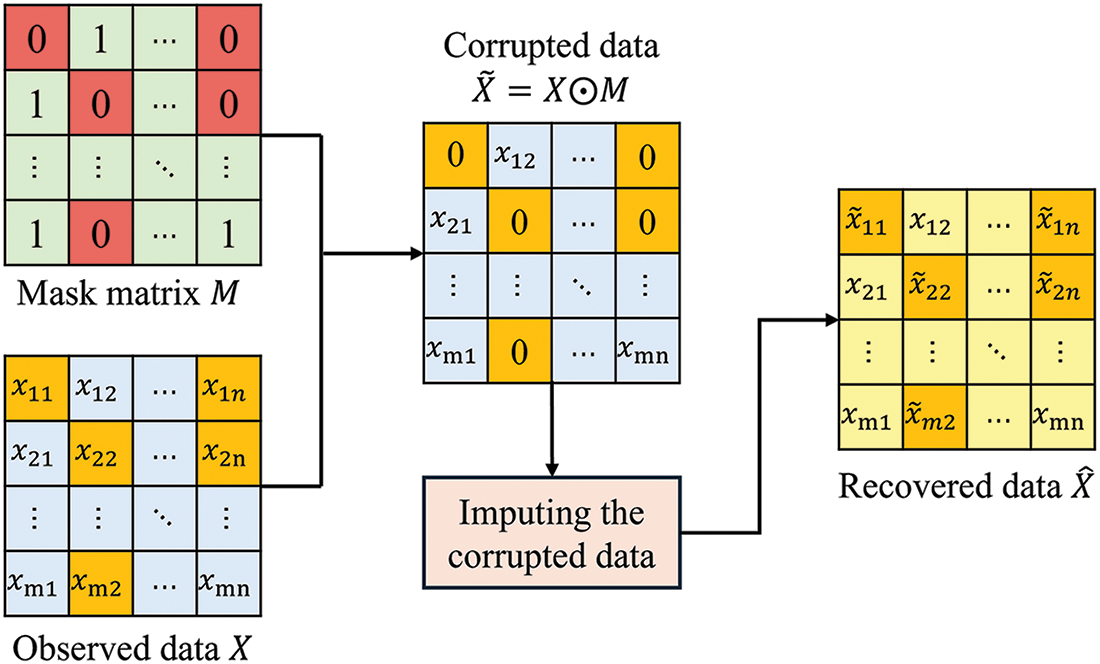
Figure 1: Data recovery process

4  TGAIN

Considering the temporal correlation of geospatial data, we introduce the LSTM network into the generative adversarial interpolation network and propose a new interpolation framework to deal with the interpolation problem of geospatial data. The general framework of TGAIN is shown in Fig. 2, where the input data are the data matrix, the random matrix, and the mask matrix. In TGAIN, we have designed two components, that is, time generator and discriminator. To forecast the missing data, we developed the internal framework of a temporal generator and a spatio-temporal discriminator, utilizing long short-term memory (LSTM) networks and convolutional neural networks (CNN), respectively, to seize temporal interdependencies. With the assistance of the temporal correlation module, the missing parts are complemented to obtain a matrix that combines the complemented and observed values. This matrix is combined with the cue matrix generated by the cue-mask fusion mechanism to produce the probability distribution estimation matrix P through the discriminator.

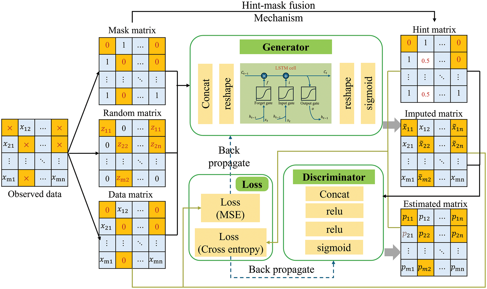
Figure 2: General framework diagram of TGAIN

Based on the architecture described above, we assume that the geospatial data matrix is X∈RN×C, M is its corresponding mask matrix, and Z is the random noise matrix. We have the following equations:

X¯=G(ℜ~, M, (1−M)⊙Z),(2)

X^=ℜ~⊙M+X¯⊙(1−M).(3)

where ⊙ denotes element-wise multiplication, X¯ is the estimated generator output, and X^ is the interpolated data. X^ is the data obtained by taking ℜ~ from a portion of the observed data and replacing each ∗ in ℜ~ with the corresponding value X¯.

The flowchart of TGAIN is depicted in Fig. 3. The TGAIN model’s architecture encompasses the following components:

•   GAIN Architecture in TGAIN: Leveraging a generative adversarial network (GAN), GAIN targets the estimation of missing data values via the generator-discriminator rivalry during adversarial training. It comprises two main components: (1) The Generator, tasked with producing complete output from input data, regardless of missing values; (2) The Discriminator, which evaluates the generator’s output to differentiate between synthetic and authentic data.

•   Role of LSTM in Integration: The TGAIN model enhances its time series data performance by incorporating a long short-term memory network (LSTM), a specialized recurrent neural network (RNN) adept at capturing long-range dependencies, within its GAIN-based generator. This integration allows TGAIN to more effectively manage geospatial data’s temporal dynamics, ensuring that the generated data is not only plausible at individual time points but also maintains continuity and coherence over time. Consequently, the LSTM-augmented generator elevates the quality of the synthesized data.

•   Cue-masked fusion matrix mechanism: This mechanism refines the generator’s training by incorporating a hint mask matrix that aids the discriminator in differentiating real from synthetic data. The process involves: (1) Generating a hint mask matrix: A binary matrix is created, where ‘1’s denote preserved real data and ‘0’s denote data filled in by the generator. This matrix is applied variably across the input and generated datasets, ensuring the generator grasps the overall data distribution; (2) Fusion: The hint mask matrix merges with both input and generated data, providing the discriminator with clues to identify synthetic vs. authentic data, thereby enhancing adversarial training efficacy; (3) Enhanced performance: The hint mask matrix allows the generator to more efficiently learn the missing data’s distribution, boosting the precision and quality of the completed data. Moreover, the fusion process challenges the discriminator, encouraging the generator to create more realistic outputs.

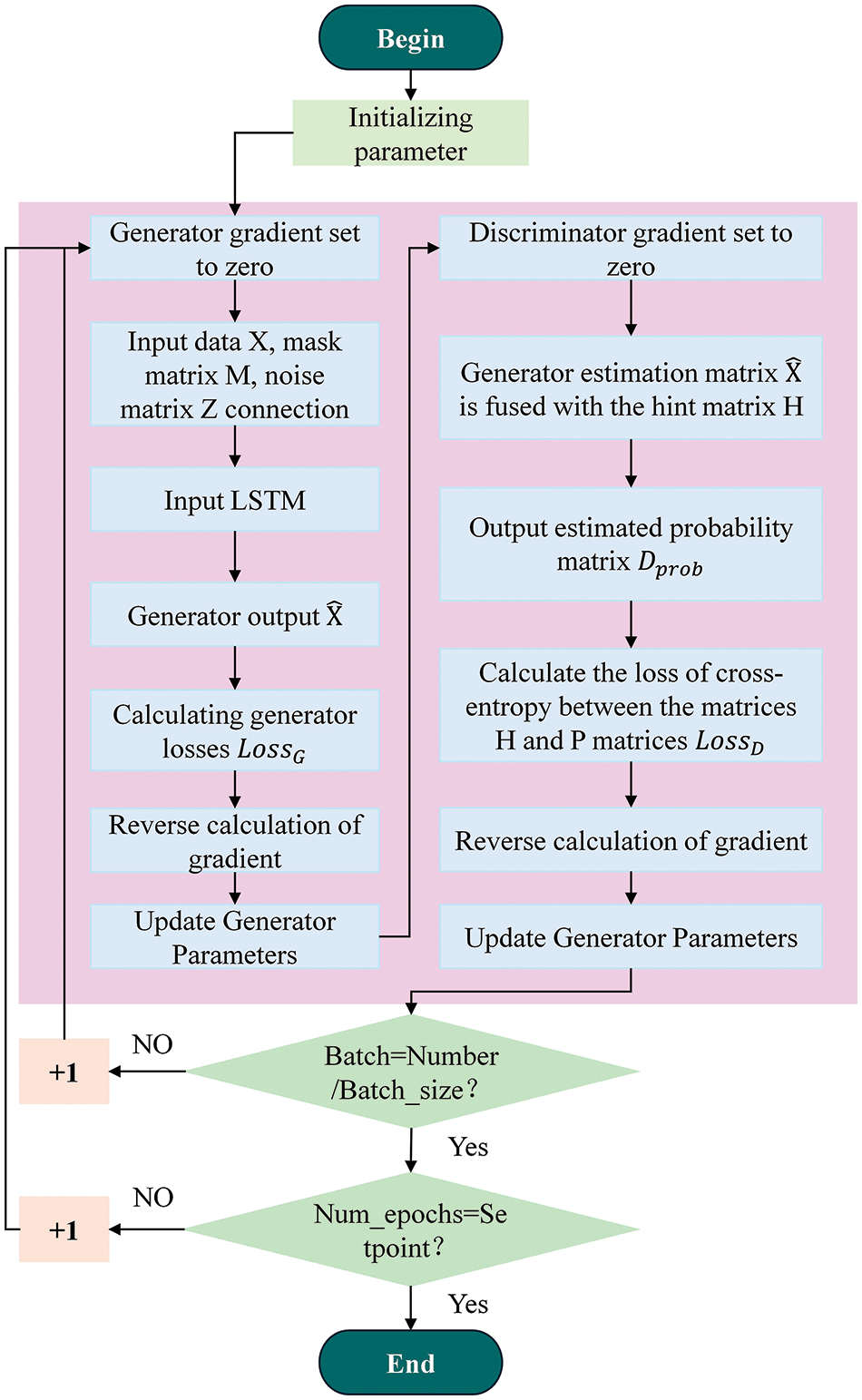
Figure 3: The flowchart of TGAIN

4.1 Generator

To capture the temporal correlation in the geospatial data, we introduce an LSTM layer into the generator. We fused the original matrix X with the random noise matrix Z according to Eq. (4) enabling the model to identify missing locations.

X∗=X⊙M+Z⊙(1−M).(4)

We then splice the input X∗ with the mask matrix M into the LSTM layer, which has the powerful ability to learn the long-term correlation of the sequence data to capture the evolutionary patterns of the spatial data. The standard LSTM architecture can be described as an encapsulated unit with several multiplication gate cells, as shown in Fig. 4.

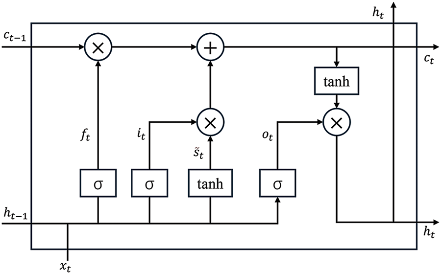
Figure 4: LSTM architecture

For a certain time step t, the LSTM unit takes the current input vector xt and the state vector of the previous time step ht−1 as input and then outputs the state vector of the current time step ht as shown in the following equations:

ft=σ(Wxfxt+Whfht−1+bf),(5)

it=σ(Wxixt+Whiht−1+bi),(6)

s~t=σ(Wxsxt+Whsht−1+bs),(7)

st=ft⊙st−1+it⊙s~t,(8)

ot=σ(Wxoxt+Whoht−1+bo),(9)

ht=ot⊙tanh⁡(sι).(10)

Here it, ft, ot, st, s~t and ht denote the input gate, forgetting gate, output gate, cell state, candidate memory and hidden state, respectively, The set {Wx, Wh, b} comprises the parameters for these cells, σ(⋅) signifies the sigmoid activation function; and ⊙ represents the element-wise multiplication.

Finally, we input the hidden state sequence into the fully connected layer to get the final result X¯ generated by the generator.

4.2 Discriminator

In the discriminator, we introduce a hint matrix H containing information about the original data and define the random variable B=(B1,…,Bn)∈{0, 1}n. Here H={0, 0.5, 1}n can be computed by M. With the help of the hint matrix H, the accuracy of the discriminator can be improved. In this paper, the hint matrix H is defined as follows:

H=B⊙M+0.5⊙(1−B).(11)

Here 0.5 is a hint value, that is, the hint parameter that we chose when designing the hint matrix to decide whether or not a certain element should be included in the hint message during the binary operation. The hint parameter provides a priori information for data recovery and helps the generator to better recover missing parts when dealing with missing data. The value was chosen through experimental adjustment and has a value interval between [0.1, 1].

We introduce the synthetic sample X^ and the hint matrix H to the discriminator to differentiate between the observed and completed portions of the sample. In contrast to traditional GAN models, the discriminator in TGAIN focuses on identifying the genuineness of the sample’s missing vs. non-missing segments, utilizing the mask matrix M as labels for this task.

Fig. 5 illustrates the discriminator’s architecture, where D∗ signifies the model parameters. In TGAIN, we configure three convolutional layers and apply a Sigmoid function to the output layer to yield a discriminative probability Dprob ranging from 0 to 1. Training aims to maximize the probability for observed data towards 1 and minimize it for missing data towards 0.

Figure 5: The structure of the discriminator

4.3 Loss Function

The optimization of TGAIN includes two components, generator loss and discriminator loss, for learning generator networks and discriminator networks. The discriminator should possess robust discriminative capabilities, whereas the generator should facilitate the discriminator in maximizing the likelihood of identifying the generator-produced data as incorrect. In this paper, the objective function of TGAIN is expressed as Eq. (12).

minG⁡maxD⁡EX^, M, H[MTlog⁡D(X^, H)+(1−MT)×log⁡(1−D(X^, H))].(12)

Here G and D denote the output of the generator and discriminator, respectively.

During the ongoing competition between the discriminator and the generator, the capabilities of both the discriminator and the generator network progressively improve. The generator becomes adept at producing samples that closely resemble authentic ones, while the discriminator increasingly struggles to differentiate between genuine and synthetic samples. Ultimately, the discriminator’s probability of making a correct judgment will settle at 0.5. The loss function for the discriminator can be expressed using cross-entropy, as depicted in the subsequent equation.

LossD=−1N×C(M⊙log⁡(D(x))+({1}−M)⊙log⁡(1−D(G(z)))).(13)

In this context, D(x) represents the discriminative probability for the actual data x, and D(G(z)) signifies the discriminative probability for the data generated by the model G(z).

The interpolation loss serves to quantify the discrepancy between the input value and the actual value for every term that is missing. The loss of interpolation is minimized when the interpolated features are close to the observed features. To adequately measure the effect of the interpolation in the missing, we use MSE to calculate the loss of the interpolation at (1−M)=1. The formula for the interpolation loss is presented in Eq. (14) as follows:

Lossimputed=∑((1−M)⊙(X^−X))2∑(1−M).(14)

However, it is not enough to rely on interpolation loss to enhance the generator. To enhance the results, the feedback from the discriminator utilized is fed back to the generator as valuable information to guide its optimization. In this paper, we combine binary cross-entropy (BCE) loss with MSE loss to formulate the generator training strategy and optimize the generation process by weighted combination. Eventually, the generator’s loss function is depicted in Eq. (15).

LossG=Lossimputed+α×−(1−M)⊙log⁡(D(G(z)))∑(1−M).(15)

In summary, the TGAIN generator and discriminator have loss functions denoted as LossD and LossG, respectively.

5  Experimental Analysis

Here, we begin by presenting the experimental datasets, setup, and metrics. Subsequently, we assess our model’s performance against four others using MAE, RMSE, MSE, MAPE, R2 and average time consumption.

5.1 Experimental Datasets

In our experiments, we select two real-world datasets, T-drive Taxi Trajectories [34] and Geolife [35], to assess model performance. We refer to all experimental datasets listed in Table 1.

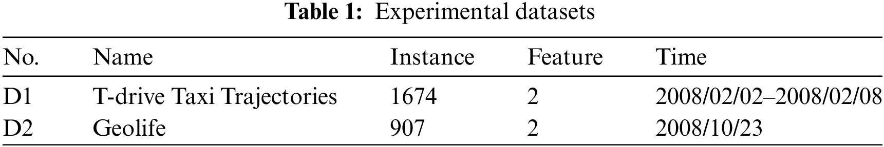
The D1 dataset consists of GPS traces from 10,357 taxis in Beijing, recorded between 02 February and 08 February 2008, with each trace including the taxi’s ID (Identity document), time, longitude, and latitude. The D2 dataset was collected from 182 users participating in the Geolife project, with GPS trajectories represented by a sequence of time-stamped points, each containing latitude, longitude, and altitude information. In this paper, we only take all the track information collected by one user as the initial data. To simulate missing data in geospatial datasets, 80% of the complete data was randomly selected as the training set, while the remaining 20% was used as the test set. The experimental data had random missing rates ranging from 10% to 70%. To ensure consistency in the experimental data and model trainability, the data was preprocessed using max-min normalization.

5.2 Experimental Setting

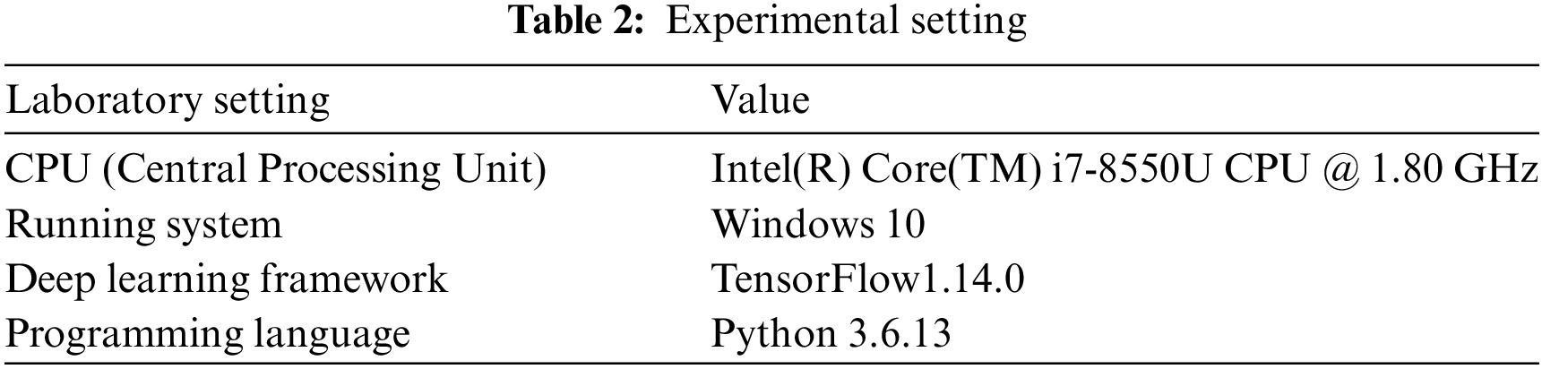
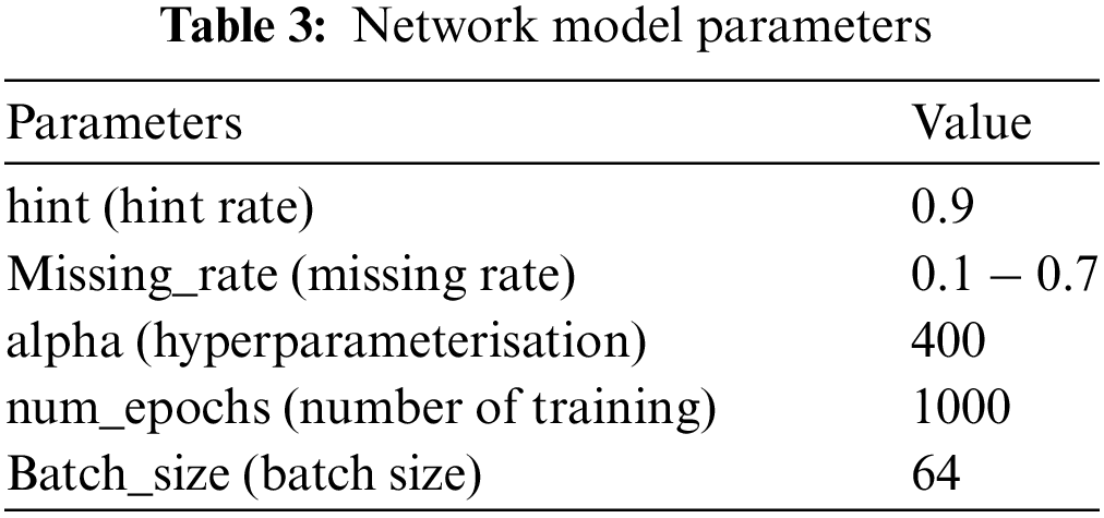
In this paper, all experiments were conducted on a personal computer with an Intel(R) Core(TM) i7-8550U CPU @ 1.80 GHz, 16.0 GB of RAM, and a 64-bit Windows 10 operating system. The specific experimental parameters are listed in Table 2, and the network model parameters are detailed in Table 3.

5.3 Metrics

In our experiments, we use MAE, RMSE, MSE, MAPE, and R2 to evaluate the data recovery accuracy of all models. The calculation of each metric is shown in the following equation, respectively:

MAE=1|1ℛ|∑i, j∈|1ℛ||Xij−X^ij|,(16)

RMSE=1|R|∑i, j∈|R|(Xij−X^ij)2,(17)

MSE=1|R|∑i, j∈|R|(Xij−X^ij)2,(18)

MAPE=100|R|∑i, j∈|R|(|Xij−X^ij|Xij),(19)

R2=1−∑i,j∈|R|(Xij−X^ij)2∑i,j∈|R|(Xij−X¯)2.(20)

where Xij is the data matrix, X^ij is the recovery matrix, |1ℛ| is the total number of data observed in the data matrix, and X¯ is the mean value of X.

5.4 Baselines

To evaluate the performance of our proposed model, in the experiments, our proposed model is compared with four classical and state-of-the-art models.

MICE [36]: MICE is a multiple interpolation based missing data filling method that uses multiple iterations and chained equations to predict missing values.

MissForest [25]: MissForest is a missing data filling method based on random forest that predicts missing values using multiple iterations and a random forest model.

GAIN [13]: GAIN is a GAN-based interpolation method that uses cue vectors to interpolate missing values.

VAE [37]: VAE is a variational autocoder that performs data filling by maximizing the likelihood probability of the input data in the latent space while minimizing the difference between the generated data and the original data.

5.5 Experimental Analysis

For all the datasets in Table 1, Figs. 6 to 10 show the MAE, RMSE, MSE, MAPE, and R2 between our proposed model and the comparison model when the data missing rate increases from 10% to 70%, respectively. And, to reflect the efficiency of our proposed model, Fig. 11 compares the average time consumption between our proposed model and the comparison model for different data missing rates.

Figure 6: MAE comparison of our model vs. others across varying data missing rates

Figure 7: RMSE comparison of our model against others under varying data missing rates

Figure 8: MSE comparison between our model and others at different data missing rates

Figure 9: MAPE comparison of our model with others across various data missing rates

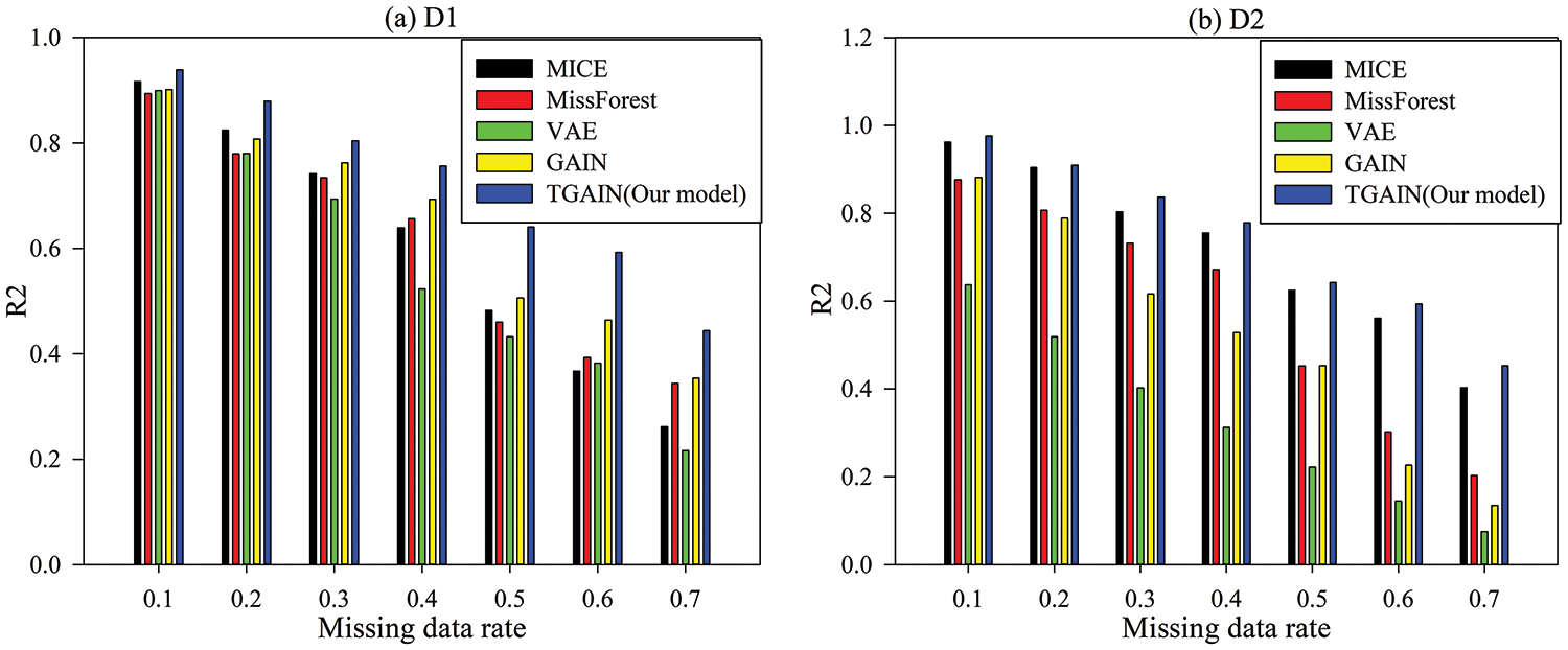
Figure 10: R2 comparison between our model and others under varying data missing rates

Figure 11: Comparison of average time-consumption between our model and other comparison models

From Figs. 6 to 9, we can see that for D2, no matter what the data missing rate is, the MAE, RMSE, MSE, and MAPE values of our proposed TGAIN model are optimal compared with other models. Especially when the data missing rate reaches more than 50%, the advantage of TGAIN is more obvious. This indicates that TGAIN has high robustness and stability when dealing with complex trajectory data recovery tasks. For dataset D1, when the data missing rate is greater than or equal to 0.5, the MAE, RMSE, MSE, and MAPE values of our proposed TGAIN model are optimal. The MAE, RMSE, MSE, MAPE values of TGAIN are optimal in all cases when the data missing rate is less than 0.5, except when the data missing rate is 0.1, the MAE and MSE values of TGAIN are greater than the MAE and MSE values of MissForest. The experimental results imply that the data recovery accuracy of our proposed TGAIN model is significantly better than that of all the compared models, especially at high data missing rates.

Fig. 10 reveals the fitability of the data of our model and other models under different data missing rates. For all experimental datasets, the R2 values of our proposed TGAIN model are significantly better than the other comparison models at different data missing rates. The difference between the R2 values of the TGAIN model and those of the other comparison models becomes more and more obvious as the data missing rate continues to increase. This also indicates that the TGAIN model has better results in fitting the data.

Combining the results of the above five evaluation indicators, it can be seen that TGAIN has the best recovery effect when the data missing rate is the lowest, and its advantage is more obvious with increasing data missing rate. In addition, the recovery error of GAIN fluctuates slightly with the increase in data missing rate but remains stable in general. However, VAE is more sensitive to the data missing rate; especially at a high data missing rate, the error increases sharply. This indicates its poor adaptability to deal with large-scale missing data. This indicates that although the data recovery effectiveness of TGAIN decreases with increasing missing rates, it is still able to adapt to different missing rates with good stability.

As can be seen in Fig. 11, for all the experimental datasets, the average time consumption of all the models increases as the missing data rate keeps increasing. However, when the data missing rate is greater than 10%, the average time consumption of our proposed TGAIN model is the smallest compared to the other four models. For all experimental data sets, only when the data missing rate is 10%, the average time consumed by our proposed TGAIN model is larger than that of the MIssForest model by approximately 6.25% and 8.42%, respectively. The results show that our proposed TGAIN model has high data recovery efficiency in addition to high data recovery accuracy.

Generally, In contrast to the comparison model, TGAIN optimizes the process of data generation through a weighted combination of binary cross-entropy loss and mean-square error loss, based on adversarial training of the generator and discriminator. This loss function design allows TGAIN to recover data more accurately. This is because TGAIN is able to better balance the realism of the generated data and the similarity to the original data during optimization, and the structure of the generative adversarial network enables TGAIN to generate high-quality missing data filling results, thus outperforming traditional non-adversarial models in terms of overall recovery accuracy. In addition, the TGAIN model introduces an LSTM layer into its architecture, which enables it to capture and exploit temporal correlations in geospatial data. This ability to process temporal dynamic information allows TGAIN to show significant advantages when recovering time series data, especially when dealing with geospatial data with spatio-temporal dependencies. The TGAIN model takes advantage of the temporal nature of the capture to enable better data recovery performance even in the face of higher missing rates. However, comparison models such as VAE and MICE fail to fully consider or effectively capture temporal correlation, resulting in a difference in recovery performance when faced with data missing rates of more than 50%.

In practical applications, the TGAIN model can maintain the accuracy of the prediction despite high missing rates. For example, for traffic flow prediction in cities, the TGAIN model is able to stably recover complete timing data by capturing the temporal correlations in the timing data, solving the problem of abnormal data recovery, and providing data support for the subsequent optimization analysis of traffic flow prediction.

6  Conclusion

As the Internet and geographic information technology advance, the collection and utilization of geospatial data have become more straightforward. However, the presence of anomalous data can significantly affect data quality and the analysis process. This paper introduces a geospatial data recovery technique known as TGAIN, which leverages a generative adversarial interpolation network (GAIN) and a long-short-term memory network (LSTM) to address the issue of anomalous data recovery within geospatial datasets. The TGAIN model combines the advantages of GAIN and LSTM by adopting the GAIN framework and embedding LSTM as a generator to capture the temporal dependence of geospatial time-series data. In addition, it also exploits the temporal correlation of geographic data to achieve accurate data recovery without the need for a complete data set. The experimental results show that, compared to the other four state-of-the-art and classical methods, the TGAIN model has significant advantages in terms of recovery accuracy and average time consumption, demonstrating its potential and effectiveness in dealing with geospatial data anomaly recovery. The TGAIN model outperforms traditional methods in terms of accuracy and robustness of data recovery, especially in maintaining a low error in the case of a high missing rate, which brings new data support for research and application in geospatial fields.

However, the TGAIN model currently relies mainly on data-driven methods for missing value completion and works better with time-dependent data. In the future, we will optimize the model structure and incorporate relevant domain knowledge (e.g., geographic laws and patterns) into the model to further enhance its applicability and efficiency.

Acknowledgement: The authors sincerely thank all the editors and anonymous reviewers for their valuable comments and suggestions, and express gratitude to all the team members who contributed to this work.

Funding Statement: This work was supported by the National Natural Science Foundation of China (No. 62002144), Ministry of Education Chunhui Plan Research Project (Nos. 202200345, HZKY20220125).

Author Contributions: Study conception and design: Lechan Yang and Li Li; Data collection: Lechan Yang and Shouming Ma; Analysis and interpretation of results: Lechan Yang and Li Li; Draft manuscript preparation: Lechan Yang, Li Li and Shouming Ma. All authors reviewed the results and approved the final version of the manuscript.

Availability of Data and Materials: The authors verify that the data backing the study’s findings can be found within the article itself.

Ethics Approval: Not applicable.

Conflicts of Interest: The authors declare that they have no conflicts of interest to report regarding the present study.

References

1. J. Rao, S. Gao, Y. Kang, and Q. Huang, “LSTM-TrajGAN: A deep learning approach to trajectory privacy protection,” 2020, arXiv:2006.10521. [Google Scholar]

2. Z. Wang, S. Zhang, and J. James, “Reconstruction of missing trajectory data: A deep learning approach,” in 2020 IEEE 23rd Int. Conf. Intell. Transp. Syst. (ITSC), Rhodes, Greece, Sep. 20–23, 2020, pp. 1–6. [Google Scholar]

3. C. Lyu, Q. -L. Lu, X. Wu, and C. Antoniou, “Tucker factorization-based tensor completion for robust traffic data imputation,” Transp. Res. Part C: Emerg. Technol., vol. 160, 2024, Art. no. 104502. doi: 10.1016/j.trc.2024.104502. [Google Scholar] [CrossRef]

4. J. Li, L. Xu, R. Li, P. Wu, and Z. Huang, “Deep spatial-temporal bi-directional residual optimisation based on tensor decomposition for traffic data imputation on urban road network,” Appl. Intell., vol. 52, no. 10, pp. 11363–11381, 2022. doi: 10.1007/s10489-021-03060-4. [Google Scholar] [CrossRef]

5. M. Lei, A. Labbe, Y. Wu, and L. Sun, “Bayesian kernelized matrix factorization for spatiotemporal traffic data imputation and kriging,” IEEE Trans. Intell. Transp. Syst., vol. 23, no. 10, pp. 18962–18974, 2022. doi: 10.1109/TITS.2022.3161792. [Google Scholar] [CrossRef]

6. A. B. Said and A. Erradi, “Spatiotemporal tensor completion for improved urban traffic imputation,” IEEE Trans. Intell. Transp. Syst., vol. 23, no. 7, pp. 6836–6849, 2021. doi: 10.1109/TITS.2021.3062999. [Google Scholar] [CrossRef]

7. X. Chen, Y. Chen, N. Saunier, and L. Sun, “Scalable low-rank tensor learning for spatiotemporal traffic data imputation,” Transp. Res. Part C: Emerg. Technol., vol. 129, 2021, Art. no. 103226. doi: 10.1016/j.trc.2021.103226. [Google Scholar] [CrossRef]

8. X. Chen, J. Xu, R. Zhou, W. Chen, J. Fang and C. Liu, “TrajVAE: A variational autoencoder model for trajectory generation,” Neurocomputing, vol. 428, pp. 332–339, 2021. doi: 10.1016/j.neucom.2020.03.120. [Google Scholar] [CrossRef]

9. L. Li, J. Zhang, Y. Wang, and B. Ran, “Missing value imputation for traffic-related time series data based on a multi-view learning method,” IEEE Trans. Intell. Transp. Syst., vol. 20, no. 8, pp. 2933–2943, 2018. doi: 10.1109/TITS.2018.2869768. [Google Scholar] [CrossRef]

10. T. Xia et al., “AttnMove: History enhanced trajectory recovery via attentional network,” in Proc. AAAI Conf. Artif. Intell., Vancouver, BC, Canada, Feb. 2–9, 2021, pp. 4494–4502. [Google Scholar]

11. Y. Shi, H. Gao, and W. Rao, “TIGAN: Trajectory imputation via generative adversarial network,” in Int. Conf. Adv. Data Min. Appl., Shenyang, China, Aug. 21–23, 2023, pp. 195–209. [Google Scholar]

12. E. Wang, M. Zhang, B. Yang, Y. Yang, and J. Wu, “Large-scale spatiotemporal fracture data completion in sparse crowdsensing,” IEEE Trans. Mob. Comput., vol. 23, no. 7, pp. 7585–7601, 2023. doi: 10.1109/TMC.2023.3339089. [Google Scholar] [CrossRef]

13. J. Yoon, J. Jordon, and M. Schaar, “GAIN: Missing data imputation using generative adversarial nets,” in Int. Conf. Mach. Learn., Stockholm, Sweden, Jul. 10–15, 2018, pp. 5689–5698. [Google Scholar]

14. S. Li et al., “Geospatial big data handling theory and methods: A review and research challenges,” ISPRS J. Photogramm. Remote Sens., vol. 115, pp. 119–133, 2016. doi: 10.1016/j.isprsjprs.2015.10.012. [Google Scholar] [CrossRef]

15. T. V. Zyl, I. Simonis, and G. McFerren, “The sensor web: Systems of sensor systems,” Int. J. Digit. Earth, vol. 2, no. 1, pp. 16–30, 2009. doi: 10.1080/17538940802439549. [Google Scholar] [CrossRef]

16. M. Duckham, Decentralized Spatial Computing: Foundations of Geosensor Networks. Berlin, Heidelberg, Germany: Springer Publishing Company, 2013. [Google Scholar]

17. A. Kealy, G. Retscher, C. K. Toth, and D. Grejner-Brzezinska, “Collaborative positioning-concepts and approaches for more robust positioning,” in XXV Int. FIG Congress, Kuala Lumpur, Malaysia, Jun. 16–21, 2014, p. 15. [Google Scholar]

18. S. Qiu, D. Pi, Y. Wang, and Y. Liu, “Novel trajectory privacy protection method against prediction attacks,” Expert. Syst. Appl., vol. 213, 2023, Art. no. 118870. doi: 10.1016/j.eswa.2022.118870. [Google Scholar] [CrossRef]

19. C. Chen, Z. Liu, S. Wan, J. Luan, and Q. Pei, “Traffic flow prediction based on deep learning in internet of vehicles,” IEEE Trans. Intell. Transp. Syst., vol. 22, no. 6, pp. 3776–3789, 2020. doi: 10.1109/TITS.2020.3025856. [Google Scholar] [CrossRef]

20. Z. Chen, Z. Gong, S. Yang, Q. Ma, and C. Kan, “Impact of extreme weather events on urban human flow: A perspective from location-based service data,” Comput. Environ. Urban Syst., vol. 83, 2020, Art. no. 101520. doi: 10.1016/j.compenvurbsys.2020.101520. [Google Scholar] [PubMed] [CrossRef]

21. Z. Cai, Y. Shu, X. Su, L. Guo, and Z. Ding, “A traffic data interpolation method for IoT sensors based on spatio-temporal dependence,” Internet Things, vol. 21, 2023, Art. no. 100648. doi: 10.1016/j.iot.2022.100648. [Google Scholar] [CrossRef]

22. M. M. Elshrif, K. Isufaj, and M. F. Mokbel, “Network-less trajectory imputation,” in Proc. 30th Int. Conf. Adv. Geograp. Inform. Syst., Seattle, WA, USA, Nov. 1–4, 2022, pp. 1–10. [Google Scholar]

23. J. Ke, S. Zhang, H. Yang, and X. Chen, “PCA-based missing information imputation for real-time crash likelihood prediction under imbalanced data,” Transportmetrica A: Transp. Sci., vol. 15, no. 2, pp. 872–895, 2019. doi: 10.1080/23249935.2018.1542414. [Google Scholar] [CrossRef]

24. F. Bashir and H. -L. Wei, “Handling missing data in multivariate time series using a vector autoregressive model-imputation (VAR-IM) algorithm,” Neurocomputing, vol. 276, pp. 23–30, 2018. doi: 10.1016/j.neucom.2017.03.097. [Google Scholar] [CrossRef]

25. D. J. Stekhoven and P. Bühlmann, “Missforest-non-parametric missing value imputation for mixed-type data,” Bioinformatics, vol. 28, no. 1, pp. 112–118, 2012. doi: 10.1093/bioinformatics/btr597. [Google Scholar] [PubMed] [CrossRef]

26. Z. Zeng, B. Liu, J. Feng, and X. Yang, “Low-rank tensor and hybrid smoothness regularization-based approach for traffic data imputation with multimodal missing,” IEEE Trans. Intell. Transp. Syst., pp. 1–13, 2024. doi: 10.1109/TITS.2024.3440011. [Google Scholar] [CrossRef]

27. A. Baggag et al., “Learning spatiotemporal latent factors of traffic via regularized tensor factorization: Imputing missing values and forecasting,” IEEE Trans. Knowl. Data Eng., vol. 33, no. 6, pp. 2573–2587, 2019. doi: 10.1109/TKDE.2019.2954868. [Google Scholar] [CrossRef]

28. Z. Che, S. Purushotham, K. Cho, D. Sontag, and Y. Liu, “Recurrent neural networks for multivariate time series with missing values,” Sci. Rep., vol. 8, no. 1, 2018, Art. no. 6085. doi: 10.1038/s41598-018-24271-9. [Google Scholar] [PubMed] [CrossRef]

29. J. Yoon, W. R. Zame, and M. Van der Schaar, “Estimating missing data in temporal data streams using multi-directional recurrent neural networks,” IEEE Trans. Biomed. Eng., vol. 66, no. 5, pp. 1477–1490, 2018. doi: 10.1109/TBME.2018.2874712. [Google Scholar] [PubMed] [CrossRef]

30. W. Cao, D. Wang, J. Li, H. Zhou, L. Li and Y. Li, “BRITS: Bidirectional recurrent imputation for time series,” in Adv. Neural Inform. Process. Syst., Montreal, QC, Canada, Dec. 3–8, 2018, pp. 1–11. [Google Scholar]

31. S. C. -X. Li, B. Jiang, and B. Marlin, “MisGAN: Learning from incomplete data with generative adversarial networks,” 2019, arXiv:1902.09599. [Google Scholar]

32. Y. Luo, Y. Zhang, X. Cai, and X. Yuan, “E2GAN: End-to-end generative adversarial network for multivariate time series imputation,” in Proc. Twenty-Eighth Int. Joint Conf. Artif. Intell., Macao, China, Aug. 10–16, 2019, pp. 3094–3100. [Google Scholar]

33. X. Miao, Y. Wu, J. Wang, Y. Gao, X. Mao and J. Yin, “Generative semi-supervised learning for multivariate time series imputation,” in Proc. AAAI Conf. Artif. Intell., Feb. 2–9, 2021, pp. 8983–8991. [Google Scholar]

34. J. Yuan, Y. Zheng, X. Xie, and G. Sun, “Driving with knowledge from the physical world,” in Proc. 17th ACM SIGKDD Int. Conf. Knowl. Discov. Data Min., San Diego, CA, USA, Aug. 21–24, 2011, pp. 316–324. [Google Scholar]

35. Y. Zheng, X. Xie, and W. -Y. Ma, “GeoLife: A collaborative social networking service among user, location and trajectory,” IEEE Data Eng. Bull., vol. 33, no. 2, pp. 32–39, 2010. [Google Scholar]

36. S. Van Buuren and K. Groothuis-Oudshoorn, “Mice: Multivariate imputation by chained equations in R,” J. Stat. Softw., vol. 45, pp. 1–67, 2011. doi: 10.18637/jss.v045.i03. [Google Scholar] [CrossRef]

37. J. T. McCoy, S. Kroon, and L. Auret, “Variational autoencoders for missing data imputation with application to a simulated milling circuit,” IFAC-PapersOnLine, vol. 51, no. 21, pp. 141–146, 2018. doi: 10.1016/j.ifacol.2018.09.406. [Google Scholar] [CrossRef]