Improving Generalization for Hyperspectral Image Classification: The Impact of Disjoint Sampling on Deep Models

1  Introduction

Hyperspectral Imaging (HSI) plays a pivotal role in various domains such as remote sensing [1], earth observation [2,3], urban planning [4], agriculture [5,6], forestry [7], target/object detection [8,9], mineral exploration [10], environmental monitoring [11,12], climate change [13] food processing, bakery products, bloodstain identification, and meat processing.

Hyperspectral (HS) remote sensing plays a crucial role in urban planning by providing detailed insights and tools for efficient and informed decision-making [14]. HS remote sensors capture and analyze high-resolution spectral data across numerous narrow and contiguous spectral bands, offering comprehensive information on the composition and characteristics of urban environments [15]. HS data enables precise identification and mapping of various urban land cover types, such as vegetation, impervious surfaces, and soil [16]. Additionally, HS Imagining (HSI) facilitates the detection and monitoring of changes in land use, vegetation health, and pollution levels within urban areas [17]. These capabilities enhance urban planners’ ability to assess the impact of urbanization, analyze urban metabolism, and evaluate the effectiveness of sustainability measures. By covering the entire processing chain, from data acquisition to analysis, HS remote sensing serves as a valuable tool for urban planners seeking a deeper understanding of urban environments and their dynamics.

HSI presents both challenges and opportunities for effective classification [18,19]. In recent years, Convolutional Neural Networks (CNNs) [20], Attention Graph [21,22], and Spatial-Spectral Transformers [23,24] have demonstrated remarkable success in various tasks, prompting researchers to explore their potential in HSI analysis [25]. However, achieving robust and reliable classification results requires careful consideration of data sampling techniques [26]. Random sampling for data splitting can lead to several issues. It can result in non-representative training, validation, and test sets, causing models to overfit or underfit. Different random splits produce inconsistent results, making it hard to draw meaningful conclusions [27]. Random sampling offers no control over data distribution, introducing bias in imbalanced datasets [28]. It hinders the reproducibility of experimental results and limits the exploration of data relationships. To address these challenges, disjoint sampling is a crucial yet often overlooked consideration when evaluating spatial-spectral Hyperspectral Image Classification (HSIC) models. As demonstrated by the works [1,22,29–33], traditional evaluations using overlapping training and test samples can lead to biased results and unfair assessments of model performance.

Even though several methodologies meticulously employ disjoint sets for training and testing their models, there’s a notable inconsistency in their approach when it comes to generating land-cover maps [22,30,32]. Specifically, many of these methods deviate from the disjoint sampling principle by utilizing the entire dataset for HSIC (Thematic Maps). This practice introduces a conflict between the reported accuracy and the methodology employed. To address this inconsistency, it is essential to advocate for the use of a disjoint test set exclusively for generating land-cover maps. By doing so, the evaluation process aligns more closely with the principles of unbiased model assessment. It ensures that the model is confronted with truly unseen data during the map generation phase, fostering a more accurate representation of its real-world performance.

Moreover, disjoint sampling is essential for training and evaluating deep models [34,35]. This method involves carefully selecting diverse and representative samples from various regions, land cover types, and environmental conditions to overcome biased or non-representative training data limitations [36]. It ensures the model learns robust features, enhancing classification performance and adaptability to unseen data. Additionally, disjoint sampling facilitates fair and accurate model evaluation by keeping training, validation, and testing samples separate [37]. Furthermore, disjoint sampling is crucial in training SOTA models for HSIC, notably for CNN and Spatial-Spectral Transformer-based models. It enhances generalization, ensures fair evaluation, and enables result interpretability. The use of disjoint training, validation, and test samples is imperative in HSIC for various reasons, such as:

Unbiased Evaluation: It is crucial to evaluate HSIC models using completely separate and disjoint data for training, validation, and testing in order to properly assess a model’s true ability to generalize to new unknown examples [1,29].

Preventing Data Leakage and Mitigating Overfitting: Maintaining disjoint samples for training, validation, and testing is crucial to obtaining an accurate evaluation of a model’s true generalization performance [22,37]. Employing disjoint subsets of the data at each stage of model development is pivotal in augmenting generalization performance. Through iterative training on distinct partitions, the model is compelled to infer underlying patterns shared across diverse examples, rather than being influenced by potentially misleading idiosyncrasies within a single fixed training sample [38,39]. This practice discourages the memorization of irrelevant characteristics specific to individual data samples. Instead, it fosters the capability to effectively process a wider range of presentations, including both seen and unseen examples.

Therefore, considering the above, this paper made the following contributions:

1.    This paper presents a novel approach for disjoint train, validation, and test splits for HSIC. Ensuring the disjoint splits eliminates data leakage between subsets, which can bias performance evaluations. The proposed technique provides a practical implementation for creating disjoint train, validation, and test splits from ground truth data. This allows researchers to obtain unbiased performance evaluations and reliable comparisons between HSIC models.

2.    By offering a standardized approach for creating evaluation splits, the proposed technique enhances the reproducibility and transparency of HSIC research. It fosters a more rigorous and standardized evaluation of classification models. The source code can be accessed at: https://github.com/mahmad00/Disjoint-Sampling-for-Hyperspectral-Image-Classification (accessed on 14 June 2024).

2  Mathematical Formulation

Let’s consider HSI composed of B spectral bands, each with a spatial resolution of H×W pixels. The HSI data cube, denoted as X∈R(H×W×B), is initially partitioned into overlapping 3D patches [24,40]. Each patch is centered at a spatial location (α,β) and covers a spatial extent of PS=S×S (PS = Patch size) pixels across all B bands. The total number of 3D patches (N) extracted from X (i.e., X∈R(S×S×B)) is given by (H−S+1)×(W−S+1). A patch located at (α,β) is represented as Pα,β and spans spatially from α−S−12 to α+S−12 in width and β−S−12 to β+S−12 in height. The labeling of these patches is determined by the label assigned to the central pixel within each patch as described in Algorithm 1.

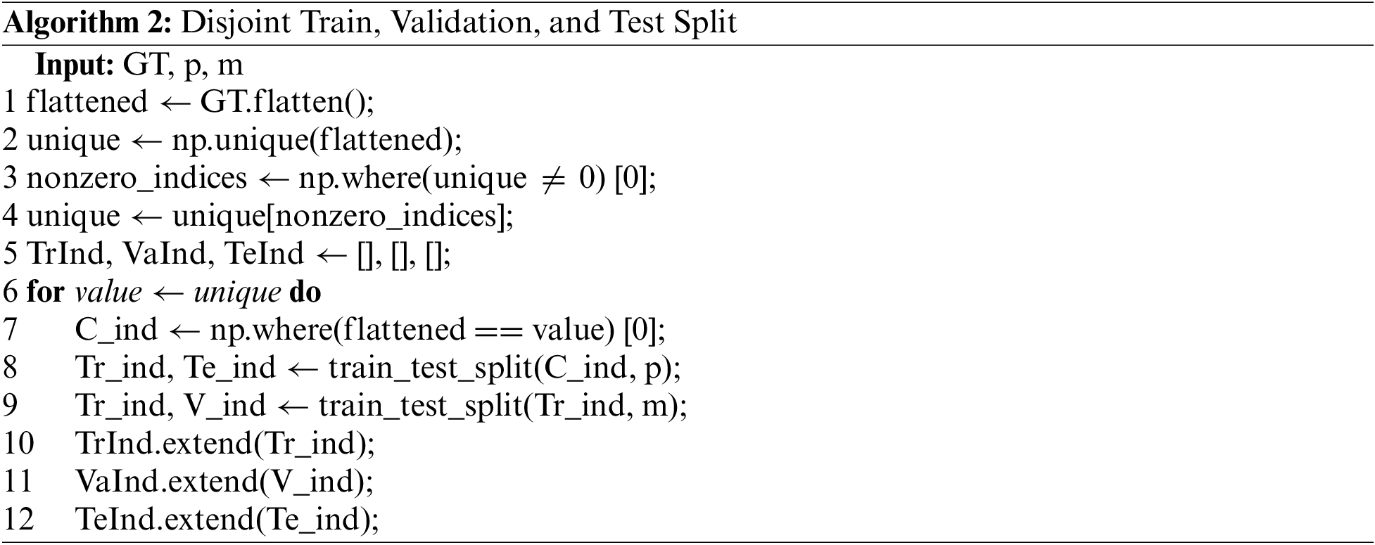
The 3D patches extracted from the HSI are used to generate separate training, validation, and test sets using the proposed splitting algorithm. The key algorithm, titled “Disjoint Train, Validation, and Test Split”, handles dividing the HSI data into the respective portions. It takes the Ground Truth (GT) labels and ratios for the test and validation sets (teRatio and vrRatio) as inputs. The unique values in the GT labels and their frequency counts are identified, excluding zeros (background pixel labels). An iterative process is then used to create disjoint training, validation, and test sets based on these unique values and their indices. The resulting indices are utilized to extract and organize the corresponding Hyperspectral cubes and labels for each set. This ensures the subsets are separate while maintaining the integrity of spectral classes during model training and evaluation. The algorithm outputs the training, validation, and test samples along with their matching class labels. This partitioning approach contributes to the robustness and reliability of the subsequent analysis.

Let us consider that n, m, and p represent the finite numbers of labeled training, validation, and test samples, respectively, selected from patch data to form the training, validation, and test sets as shown in Eqs. (1)–(3):

DTR=(xi,yi)i=1n(1)

DV=(xi,yi)i=1m(2)

DTE=(xi,yi)i=1p(3)

where n and m are the total number of training and validation samples. The remaining p samples constitute the test set. It is important to note that the intersection of the training set, validation set, and test set is an empty set (ϕ), ensuring the distinctiveness of the samples in each set as shown in Algorithm 2, Fig. 1 and Eq. (4).

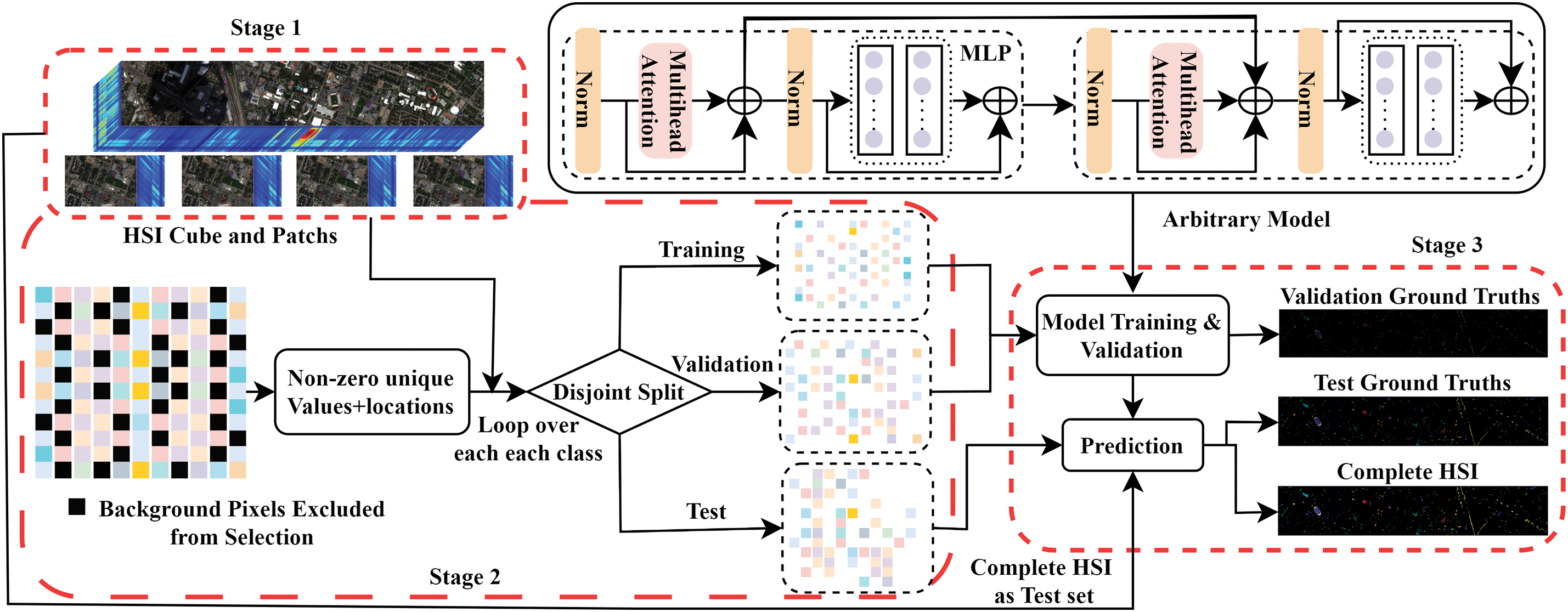
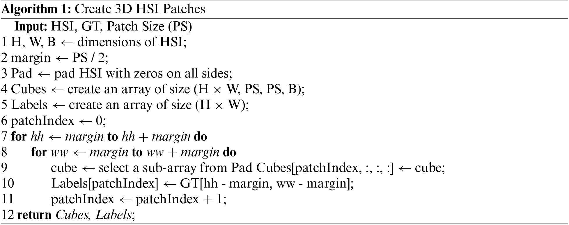
Figure 1: Initially, the HSI cube is divided into overlapping 3D patches, as detailed in Algorithm 1 and Stage 1. Each patch is centered at a spatial point and spans a PS=S×S pixel extent across all spectral bands. These patches are then utilized in Algorithm 2 to create disjoint training, validation, and test splits based on the geographical locations of the HSI samples, as outlined in Stage 2. The selected samples are fed into various models for feature learning and optimization. The processed features are subsequently passed through a fully connected layer for classification, and the softmax function is applied to generate class probability distributions. These distributions are used to create the final ground truth maps for the disjoint validation, disjoint test, and full HSI test sets, as illustrated in Stage 3. The red dotted lines delineate the stages in the proposed workflow

DTR∩DV∩DTE=ϕ(4)

As shown in Fig. 1, Stage 1: 3D Patch Extraction: The HSI cube is initially divided into overlapping 3D patches. Each patch is centered at a spatial point and spans a PS=S×S pixel extent across all spectral bands. This process is outlined in Algorithm 1. Stage 2: Data Splitting: The extracted patches are used in Algorithm 2 to create disjoint training, validation, and test splits. This splitting is based on the geographical locations of the HSI samples, ensuring that each set covers distinct areas. Stage 3: Feature Learning and Classification: The samples from each split (training, validation, and test) are fed into various models for feature learning and optimization. The learned features are passed through a fully connected layer for classification. The softmax function is then applied to generate class probability distributions. The class probability distributions are used to generate the final ground truth maps for the disjoint validation set, disjoint test set, and the full HSI test set. Each of these stages is marked with red dotted lines in Fig. 1, facilitating a clear and systematic replication of the workflow.

The above disjoint samples (as explained in Algorithm 2) are then processed by the baseline 2D, 3D CNN, and Spatial-Spectral Transformer models [41,42]. In a 2D CNN, the input data undergoes convolution with a 2D kernel function, resulting in the computation of the dot product between the input and the kernel function. The kernel is then applied in a strided manner over the input to cover the entire spatial dimension. Subsequently, the convolved features are subjected to an activation function, which introduces non-linearity into the model, aiding in the learning of non-linear features from the data. For 2D convolution, the activation value of the jth feature map at spatial location (x,y) in the ith layer, denoted by vi,jx,y, can be expressed as shown in Eq. (5).

vi,jx,y=ℱ(∑τ=1dl−1∑ρ=−γγ∑σ=−δδwi,j,τσ,ρ×vi−1,τx+σ,y+ρ+bi,j)(5)

where ℱ represents the activation function, dl−1 signifies the number of feature maps at the (l−1)th layer, while the depth of the kernel wi,j pertains to the jth feature map at the ith layer. Additionally, bi,j denotes the bias parameter for the jth feature map at the ith layer, with 2γ+1 and 2σ+1 representing the width and height of the kernel, respectively. In contrast, the 3D convolutional process initially calculates the sum of the dot product between input patches and the 3D kernel function, wherein the 3D input patches undergo convolution with the 3D kernel function [40,43]. Subsequently, these feature maps are subjected to an activation function to introduce non-linearity. The Hybrid model generates feature maps of the 3D convolutional layer by applying the 3D kernel function across B spectral bands, which are extracted post-dimensionality reduction, in the input layer. For the 3D convolutional process, the activation value at spatial location (x,y,z) in the ith layer and jth feature map can be expressed as in Eq. (6):

vi,jx,y=ℱ(∑τ=1dl−1∑λ=−vv∑ρ=−γγ∑σ=−δδwi,j,τσ,ρ,λ×vi−1,τx+σ,y+ρ,z+λ+bi,j)(6)

where all the parameters are the same as defined in Eq. (5) except 2v+1 which is the depth of the 3D kernel along a spectral dimension.

For the Spatial-Spectral Transformer model [44–46], consider fi,j∈RN×D as the input tensor fed into the Transformer, where N signifies the number of patches, and D denotes the dimensionality of each patch post convolutional processing. This encoding process is fused with the input embeddings, enriching the model with spatial arrangement details. At the core of the Transformer lies its foundational architecture, the encoder, which comprises multiple layers housing multimodal attention mechanisms and a feed-forward network. The attention mechanism assumes a pivotal role in facilitating the model’s ability to capture intricate relationships between diverse patches. More specifically, for a given input vi,j, each layer within the Transformer encoder encompasses layer normalization, cross attention, and Multi-layer Perceptron (MLP).

Given a query matrix Q∈ℛ(nq×dk), key matrix K∈ℛ(nk×dk), value matrix V∈ℛ(nv×dv), and mask matrix M∈ℛ(nq×nk), where nq,nk,nv, and dv represent the number of queries, keys, values, the dimensionality of keys/queries, and the dimensionality of values, respectively. Lets define the weight matrices for each head i as 𝒲iQ∈ℛdmodel×dk, 𝒲iK∈ℛdmodel×dk, and 𝒲iV∈ℛdmodel×dv. Apply linear transformation as: Qi=Q×𝒲iQ, Ki=K×𝒲iK, and Vi=V×𝒲iV. Later compute the attention scores for each head and apply the Softmax to compute the weighted sum of the values as shown in Eq. (7).

AttenW=Softmax(Qi×KiTdk+M)×V(7)

Then calculate the concatenate the outputs from all heads as ℋ=Concat(ℋ1,ℋ2,⋮,ℋh) and apply a final linear transformation as ℋattl. Then given an input x∈ℛdmodel, layer normalization is computed as shown in Eq. (8).

Norm(x)=x−μν2+ηγ+λ(8)

where μ is the mean and ν2 is the variance of x, η is a small constant for numerical stability and γ and λ are learnable parameters. Later the information is processed through MLP that consists of two linear transformations with a ReLU activation function as shown in (9).

MLP(x)=ReLu(x𝒲1+b1)𝒲2+b2(9)

where 𝒲1∈ℛdmodel×dff, b1∈ℛdff, 𝒲2∈ℛdff×dmodel, and b2∈ℛdmodel. The output of the multi-head self-attention Hattl is added to the input and normalized as presented in Eq. (10).

ℋ^attl=Norm(ℋattl⊕ℋ(l−1))(10)

Eq. (10) adds the attention output ℋattl to the previous layer’s output ℋatt(l−1) and normalizes the results.

ℋMLPl=MLP(ℋ^attl)(11)

Eq. (11) computes the output of the attention mechanism in the l-th layer through an MLP. The MLP consists of two linear layers with a ReLU activation function applied between them. The output of the MLP is added to the normalized attention output and normalized again as:

ℋl=Norm(ℋMLPl⊕ℋ^attl)(12)

Eq. (12) adds the output ℋMLPl to the normalized attention output and then normalizes the result once more. Afterward, ℋl is flattened into (ℋl,(b×h×w,1)), where b, h, and w denote the batch size, height, and width, respectively. Finally, a Softmax function is utilized to produce the GT maps.

3  Experimental Results and Discussion

3.1 Experimental Datasets

In order to highlight the importance and the proposed procedure of disjoint sampling in HSIC, the following datasets are used.

The University of Houston: The University of Houston dataset consists of 144 spectral bands spanning wavelengths from 380 to 1050 nm, the dataset encompasses an imaged spatial region measuring 349×1905 pixels at a resolution of 2.5 meters per pixel. Additionally, the dataset annotates 15 labeled classes pertaining to urban land use and land cover types. The disjoint train, validation, and test samples are presented in Table 1 and Fig. 2.

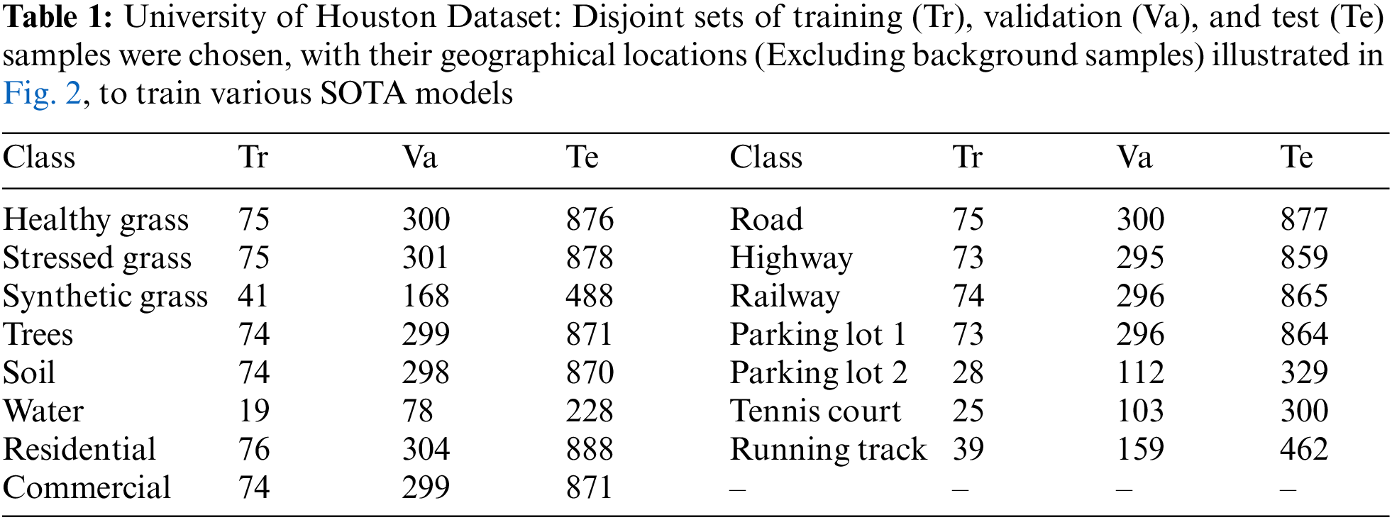
Figure 2: The University of Houston Dataset: Geographical locations of the disjoint train, validation, and test samples presented in Table 1

Indian Pines: The Indian Pines dataset was collected by the Airborne Visible/Infrared Imaging Spectrometer (AVIRIS) over an agricultural site in Northwestern Indiana. It consists of 145×145 pixels with spectral information across 224 narrow bands ranging from 0.4 to 2.5 micrometers. The major land cover classes in the dataset included agricultural land, forest, highways, rail lines, low-density housing, and built structures separated by smaller roads. Crops such as corn and soybeans covered less than 5% of typical growing areas as the June image showed early stages of development. Ground truths designate 16 non-mutually exclusive classes. The number of bands was reduced to 200 by removing wavelengths associated with water absorption. The disjoint train, validation, and test samples are presented in Table 2 and Fig. 3.

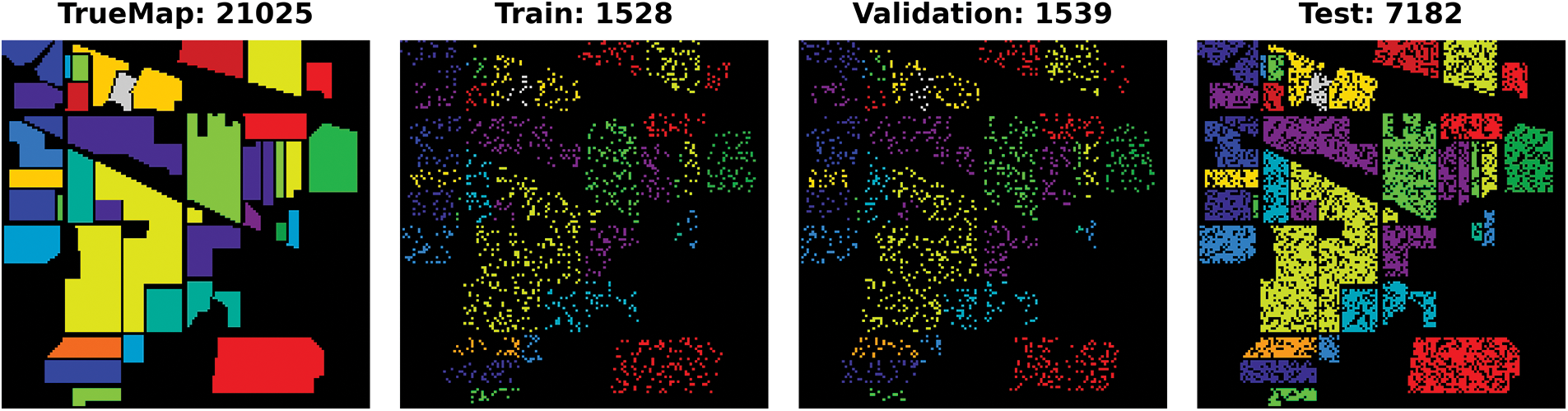
Figure 3: Indian Pines: Geographical locations of the disjoint train, validation, and test samples presented in Table 2

Pavia University: The Pavia University dataset was captured using the Reflective Optics System Imaging Spectrometer (ROSIS), this dataset consists of an image with 610×340 pixels and 115 spectral bands. It has 9 classes of urban materials-including asphalt, meadows, gravel, trees, metal sheets, bare soil, bitumen, brick, and shadows-comprising 42,776 labeled samples in total. The disjoint train, validation, and test samples are presented in Table 3 and Fig. 4.

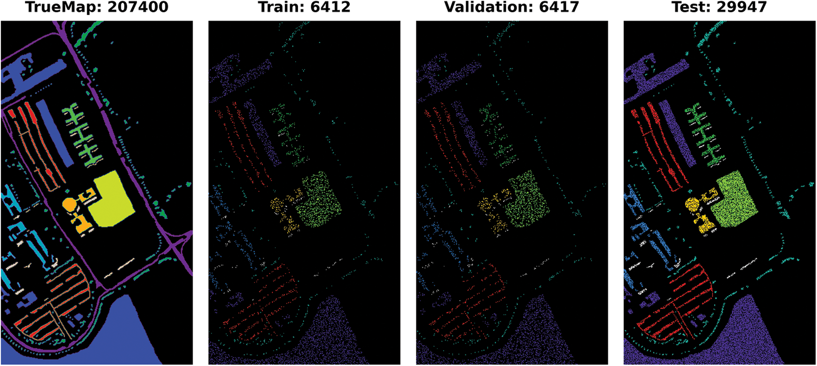
Figure 4: Pavia University Dataset: Geographical locations of the disjoint train, validation, and test samples presented in Table 3

Salinas: The Salinas dataset is collected using the 224-band AVIRIS sensor over Salinas Valley, California, this dataset is characterized by high spatial resolution at 3.7 m per pixel. The study area encompasses 512 lines by 217 samples after removing 20 bands obscured by water absorption. Land cover types within the dataset include vegetables, bare soils, and vineyard fields. The Salinas ground truth annotates 16 classes. The disjoint train, validation, and test samples are presented in Table 4 and Fig. 5.

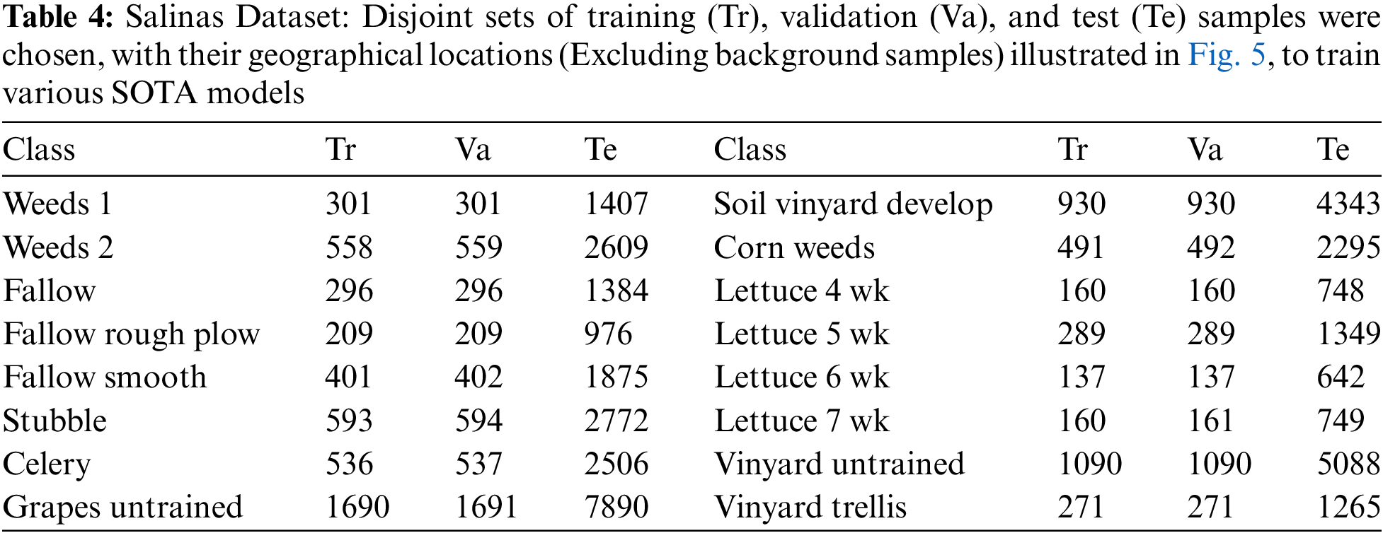
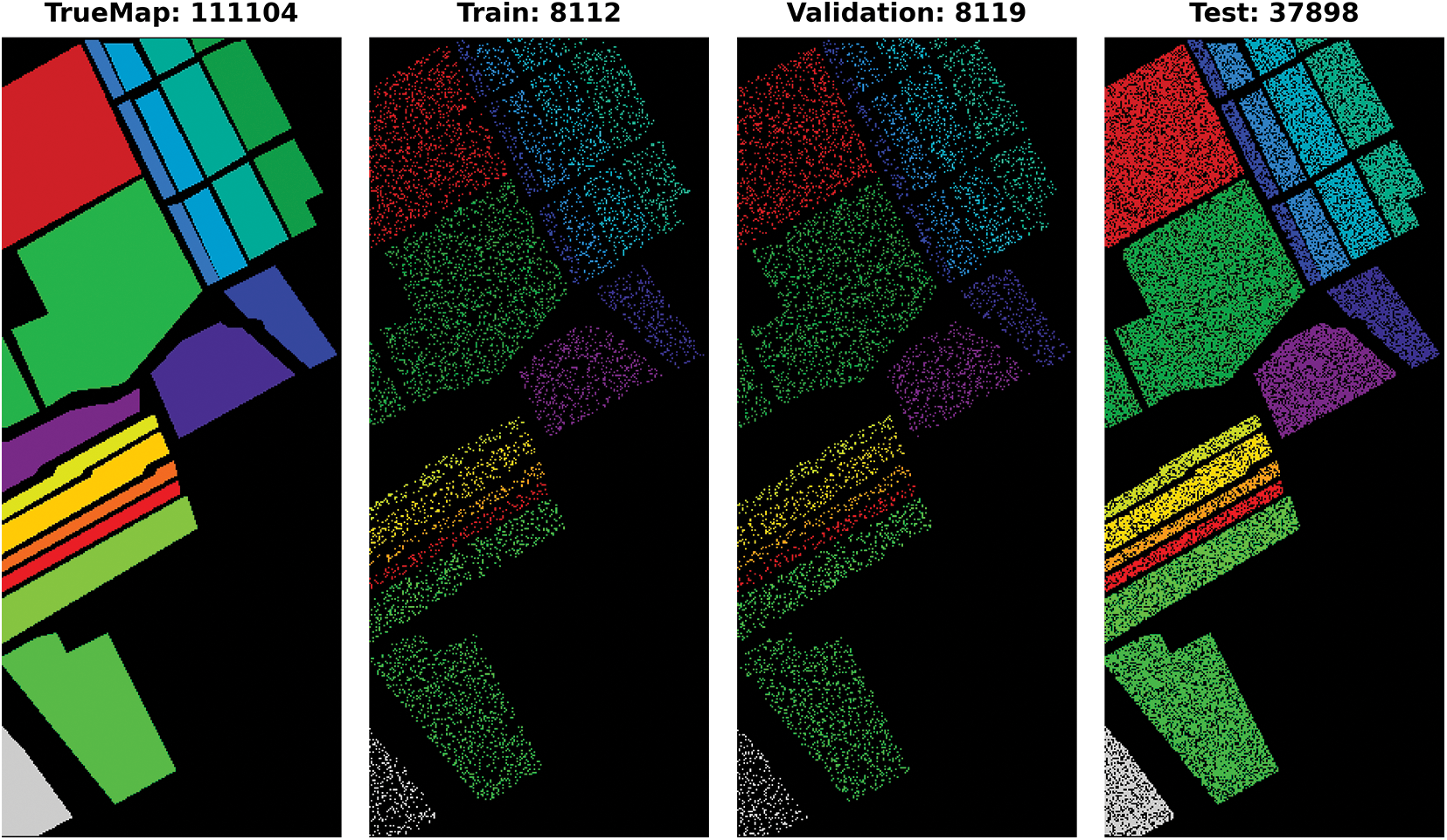
Figure 5: Salinas Dataset: Geographical locations of the disjoint train, validation, and test samples presented in Table 4

Botswana: The NASA EO-1 satellite acquired Hyperspectral imagery of the Okavango Delta region in Botswana from 2001–2004 using the Hyperion sensor to collect 30 m resolution data across 242 bands from 400–2500 nm over a 7.7 km strip. The data analyzed from 31 May, 2001, consisted of observations of 14 land cover classes representing seasonal swamps, occasional swamps, and drier woodlands in the distal delta region after preprocessing removed uncalibrated and noisy bands covering water absorption and retaining 145 bands. The disjoint train, validation, and test samples are presented in Table 5 and Fig. 6.

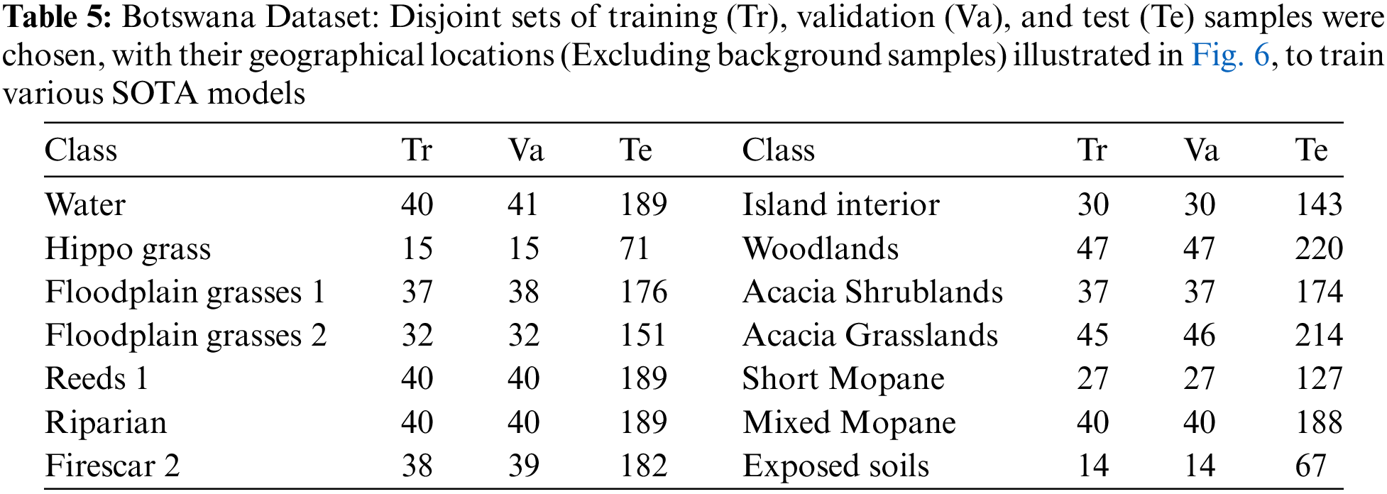
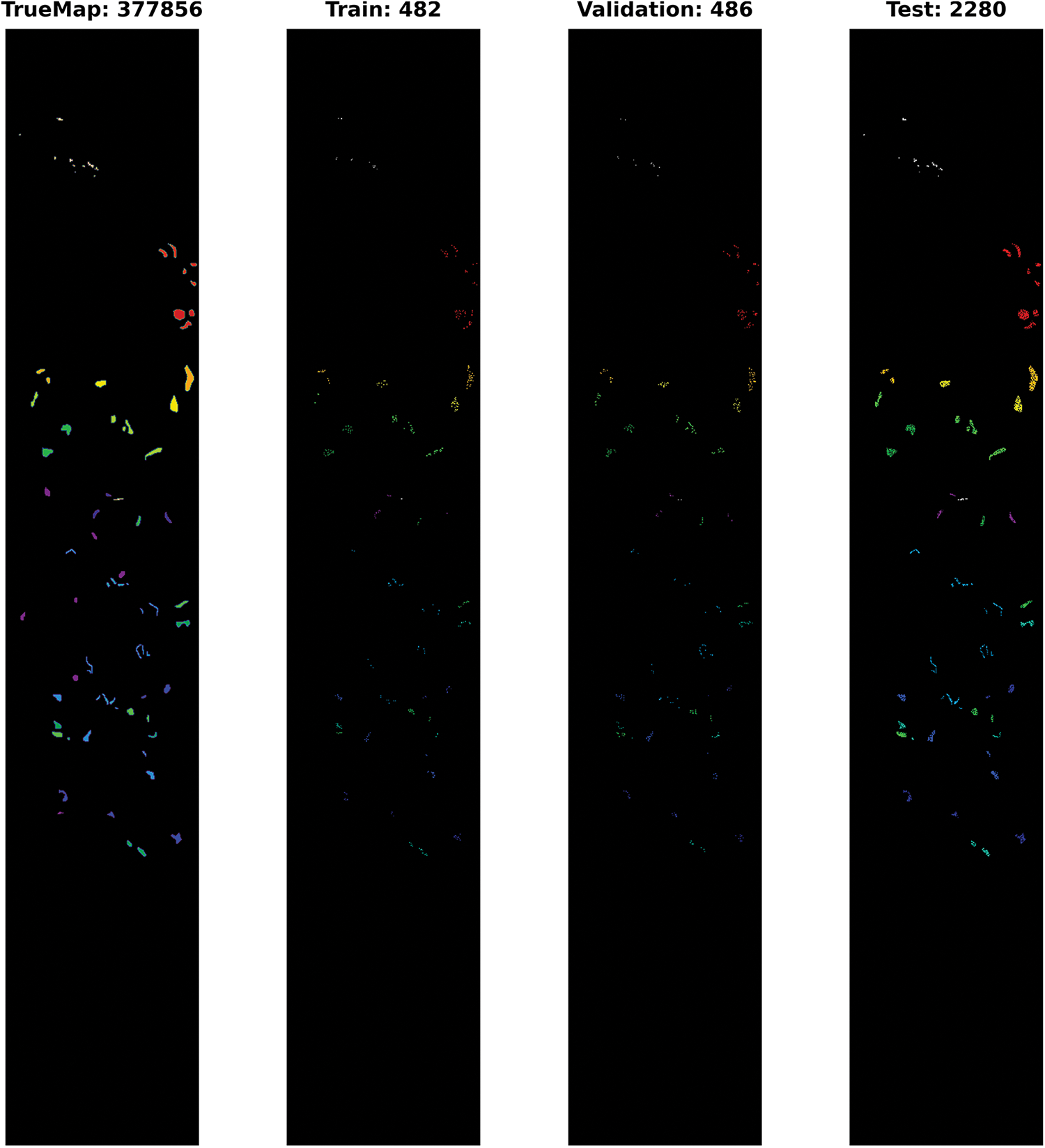
Figure 6: Botswana Dataset: Geographical locations of the disjoint train, validation, and test samples presented in Table 5

3.2 Experimental Settings

This section presents comprehensive experimental settings for various deep learning models, including 3D CNN [20], Hybrid Inception Net [47], 3D Inception Net [48], 2D Inception Net [49], 2D CNN [50], Hybrid CNN [51], Attention Graph CNN [22]. Spatial-spectral Transformer [24]. Prior to training, 3D overlapped patches are extracted using an 8×8 window size, as outlined in Algorithm 1. All models in this study are trained using the Adam optimizer with a learning rate of 0.0001, a decay rate of 1e-06, and a batch size of 56 for 50 epochs. The loss and accuracy trend is presented in Fig. 7 for all the competing methods.

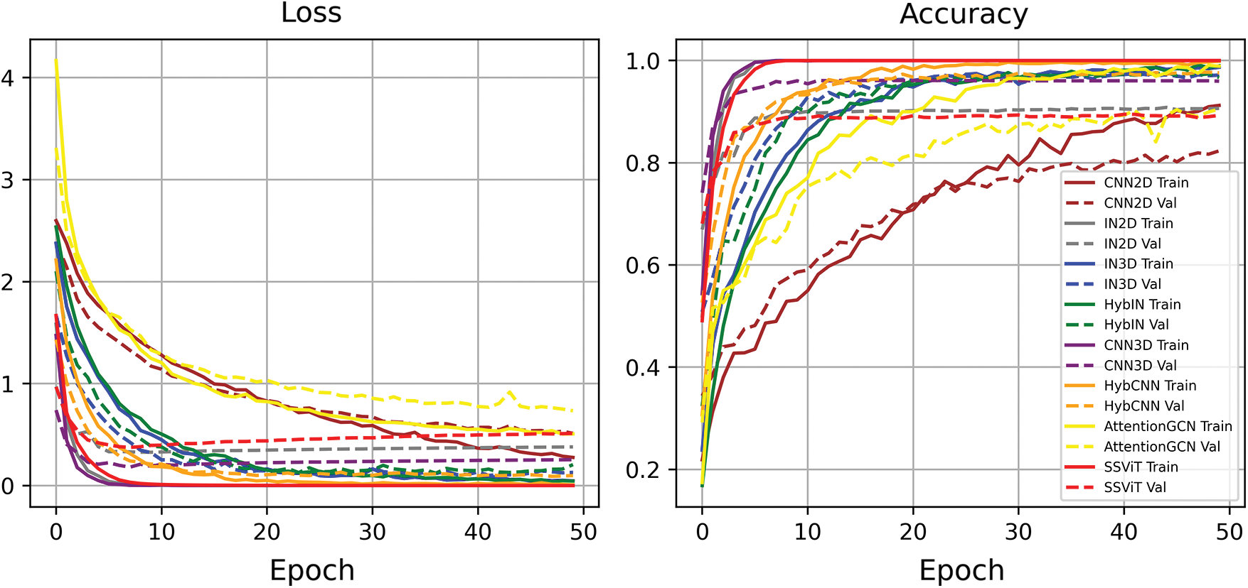
Figure 7: Loss and Accuracy trends for all the competing methods for Indian Pines dataset

All evaluations were conducted on a Google Colab, using a Jupyter Notebook. Colab works on online resources and requires a fast and stable internet connection. Colab works on a Python 3 notebook with a graphic processing unit (GPU) for data analysis, offering 25 GB of random access memory (RAM) and 358 GB of storage.

All the competing methods are tested with a patch size of 8×8, using the 15 most informative bands selected through principal component analysis. The dataset is split into 70% test samples, with the remaining 30% equally divided into training and validation sets (15% each). For effective learning, all models are trained using the Adam optimizer with a learning rate of 0.0001 and a decay of 1e−06 over 50 epochs, with a batch size of 56.

The 2D CNN model is trained using four convolutional layers with kernel sizes of (3×3×8,16,32,64) and the same padding with (8,16,32,64) number of filters, respectively. Following the convolutional layers, two dense layers are utilized with a dropout rate of 0.4%. Finally, a classification layer with Softmax is added with the number of output units corresponding to the number of classes in the dataset. The 3D CNN model is trained using four convolutional layers with kernel sizes of (3×3×7,5,3,3) with (8,16,32,64) number of filters, respectively. Following the convolutional layers, two dense layers are utilized and finally, a classification layer with Softmax is added with the number of output units corresponding to the number of classes in the dataset. The Hybrid CNN model is trained using three 3D convolutional layers with kernel sizes of (3×3×7,5,3), followed by a reshaped layer to transform the features into 2D to learn spatial features using (3×3) kernel with 64 filters. Following the convolutional layers, two dense layers are utilized with a dropout rate of 0.4%. Finally, a classification layer with Softmax is added with the number of output units corresponding to the number of classes in the dataset.

The 2D Inception Net architecture consists of three blocks with the following configurations. In the first block, three 2D convolutional layers are used. The first layer employs a (1×1) kernel with 30 filters, the second layer uses a (3×3) kernel with 20 filters, and the third layer utilizes a (1×1) kernel with 10 filters. In the second block, three 2D convolutional layers are utilized. The first layer has a (1×1) kernel with 40 filters, the second layer employs a (5×5) kernel with 20 filters, and the third layer uses a (1×1) kernel with 10 filters. The third block begins with a 2D max pooling operation using a (3×3) kernel and the same padding. This is followed by two 2D convolutional layers with (1×1) kernels and the same padding. The filters for these layers are set to 20 and 10, respectively. Afterward, the outputs from all three blocks are concatenated, and a convolutional layer with a (1×1) kernel and 128 filters is applied. Following the convolutional layer, two dense layers are deployed. Finally, a classification layer with Softmax is added with the number of output units corresponding to the number of classes in the dataset.

The 3D Inception Net architecture consists of three blocks with the following configurations. In the first block, three 3D convolutional layers are used. The first layer employs a (5×5×7) kernel with 30 filters, the second layer uses a (3×3×5) kernel with 20 filters, and the third layer utilizes a (3×3×3) kernel with 10 filters and the same padding in all three layers. In the second block, three 3D convolutional layers are utilized. The first layer has a (5×5×7) kernel with 40 filters, the second layer employs a (3×3×5) kernel with 20 filters, and the third layer uses a (3×3×3) kernel with 10 filters and the same padding in all three layers. The third block begins with three 3D convolutional layers with (5×5×7) kernel with 60 filters, the second layer uses a (3×3×5) kernel with 30 filters, and the third layer utilizes a (3×3×3) kernel with 10 filters and the same padding in all three layers. Afterward, the outputs from all three blocks are concatenated, and a convolutional layer with a (1×1×1) kernel and 128 filters is applied. Following the convolutional layer, two dense layers are deployed with a 0.4% dropout rate. Finally, a classification layer with Softmax is added with the number of output units corresponding to the number of classes in the dataset.

The hybrid Inception Net architecture consists of three blocks with the following configurations. In the first block, three 3D convolutional layers are used. The first layer has a (5×5×7) kernel with 30 filters, the second layer uses a (3×3×5) kernel with 20 filters, and the third layer employs a (3×3×3) kernel with 10 filters. The same padding is applied in all three layers. Following the convolutional layer, a reshaped layer is used to convert the features from 3D to 2D. Next, a 2D max-pooling layer with a (3×3) filter is applied, followed by three 2D convolutional layers. Each of these layers uses a (1×1) kernel with 16, 32, and 64 filters, respectively. The same padding is used for all three layers. The same configuration is repeated for the second and third blocks, with the numbers of filters set to 40, 20, and 10 for the 3D convolutional layers, and 16, 32, and 64 for the 2D convolutional layers in the second block, and 60, 30, and 10 for the 3D convolutional layers, and 16, 32, and 64 for the 2D convolutional layers in the third block, respectively. Afterward, the outputs from all three blocks are concatenated, and a convolutional layer with a (1×1×1) kernel and 128 filters is applied. Following the convolutional layer, two dense layers are deployed with a 0.4% dropout rate. Finally, a classification layer with Softmax is added with the number of output units corresponding to the number of classes in the dataset.

The Attention Graph CNN [22] and Spatial-Spectral Transformer [24] models are trained according to the settings specified in their respective papers. The Transformer model, in particular, is used without the wavelet transformation and consists of 4 layers with 8 heads to compute the final maps. A dropout rate of 0.1 is applied to the classification layers. For more detailed information, please refer to the original papers.

3.3 Qualitative and Quantitative Results and Discussion

This section provides a detailed exploration of experimental results in comparison to the state-of-the-art (SOTA) works published in recent years. While many recent research endeavors present extensive experimental outcomes to highlight the strengths and weaknesses of their approaches, it is noteworthy that the experimental results in the literature may follow diverse protocols. For instance, the selection of training, validation, and test samples might be randomly done, and the percentage distribution may be identical. However, there could be variations in the geographical locations of each model, as these models may have undergone training, validation, and testing at different times. Comparative models may have been executed in multiple instances, either sequentially or in parallel, introducing a new set of training, validation, and test samples with the same number or percentage. Consequently, to ensure a fair comparison between the works proposed in the literature and the current study, it is imperative to employ identical experimental settings and execute them with the same set of training, validation, and test samples. This approach ensures a consistent and unbiased evaluation of the proposed methodologies against existing benchmarks.

A prevalent concern in the majority of recent literature is the presence of overlapping training and test samples. When training and validation samples are randomly selected, with or without considering the point mentioned earlier, the data split often includes overlapping samples. This situation introduces bias to the model, as overlapping implies the model has already encountered the training and validation samples, leading to inflated accuracy metrics. To prevent this issue, this study ensures that, despite the random selection of samples, the intersection between training, test, and validation samples remains consistently empty for all competing methods. This measure aims to maintain the integrity of the model evaluation process and uphold the reliability of accuracy assessments.

To ensure a robust and fair evaluation, the datasets are split into disjoint training, validation, and test sets. Following the proposed method, we begin by dividing the HSI dataset into disjoint training, validation, and test sets. Each model is then trained on the training set and tuned on the validation set to optimize performance. Subsequently, the models are evaluated on the disjoint test set and the complete HSI dataset to assess their generalization capabilities. The experimental results demonstrate the effectiveness of the proposed method in improving the classification accuracy of HSIC as shown in Tables 6–10 and Figs. 8–12. Among the deep learning models considered, 3D CNN [20] and Hybrid Inception Net [47] achieve the highest classification accuracy, indicating their suitability for HSIC. Additionally, the results highlight the importance of using a large and diverse training dataset to achieve optimal performance.

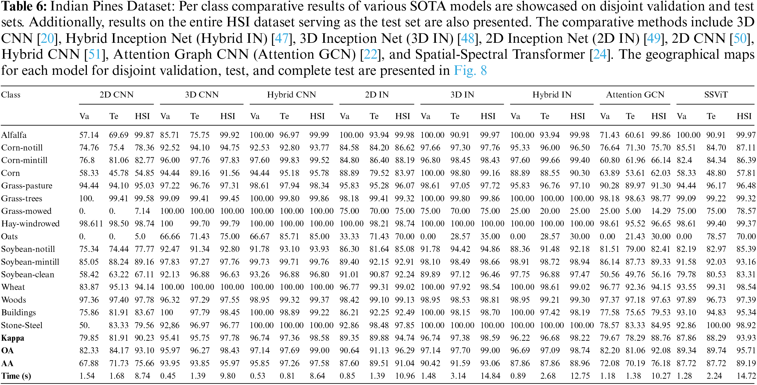
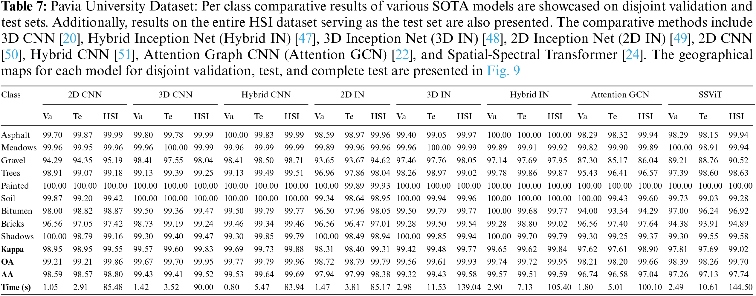
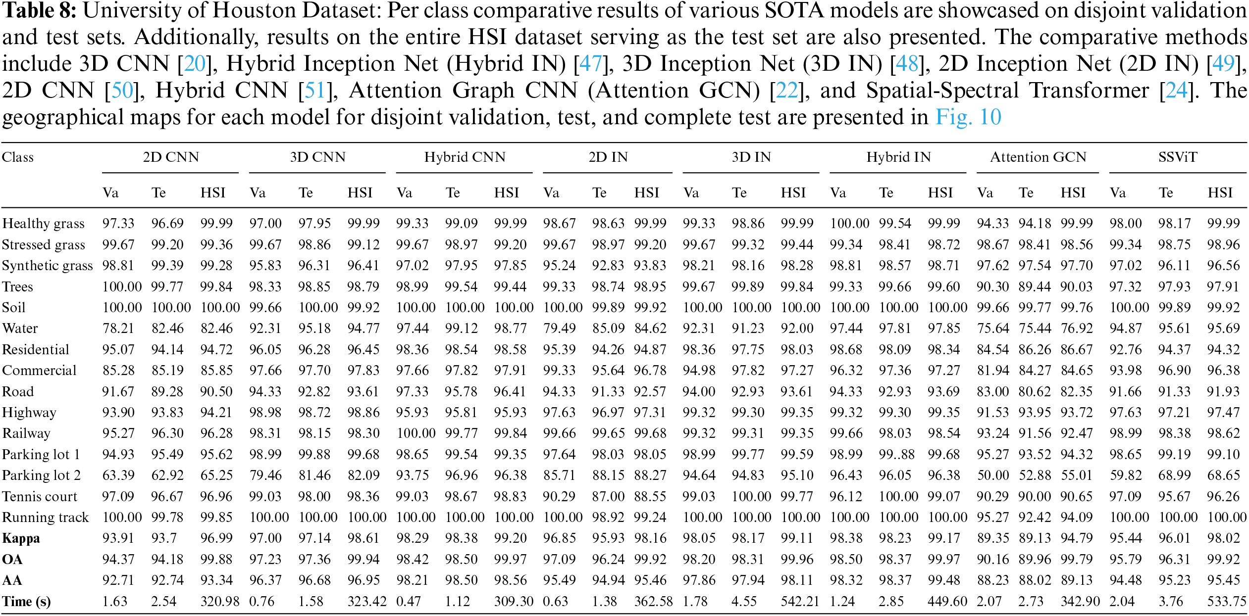
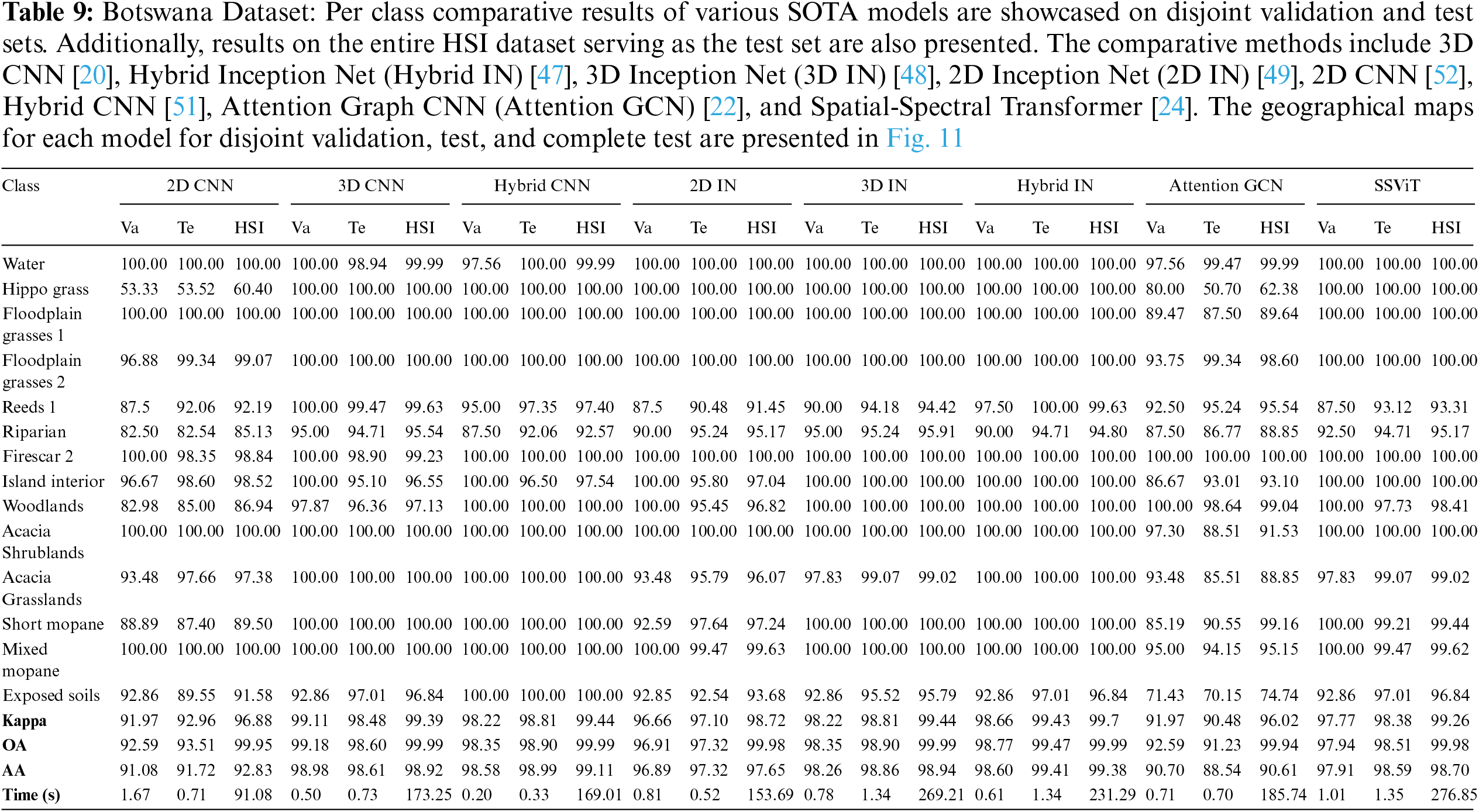
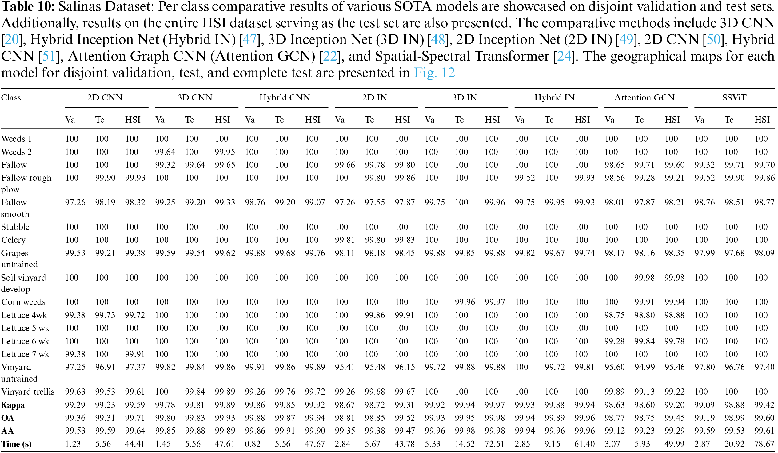
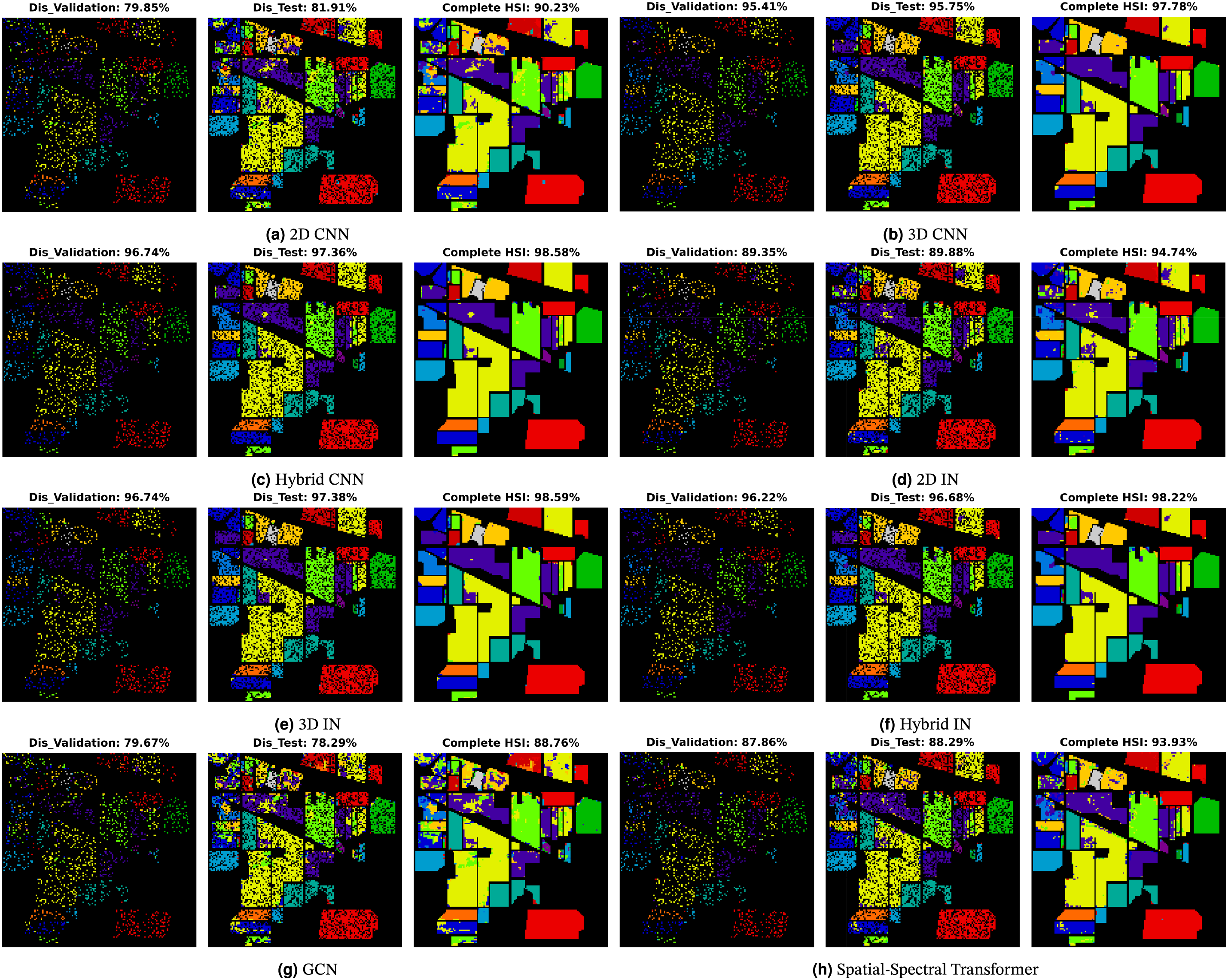
Figure 8: Indian Pines Dataset: Land cover maps for disjoint validation, test, and the entire HSI used as a test set are provided. Comprehensive class-wise results can be found in Table 6

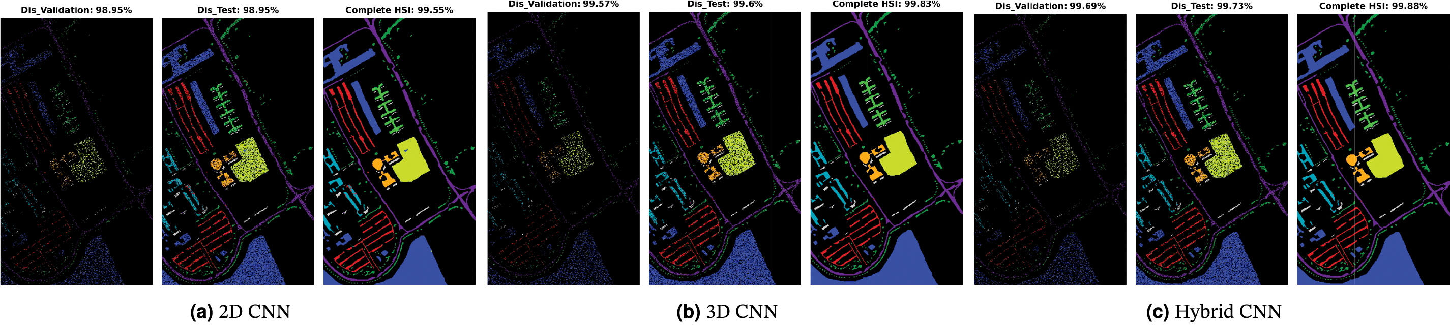
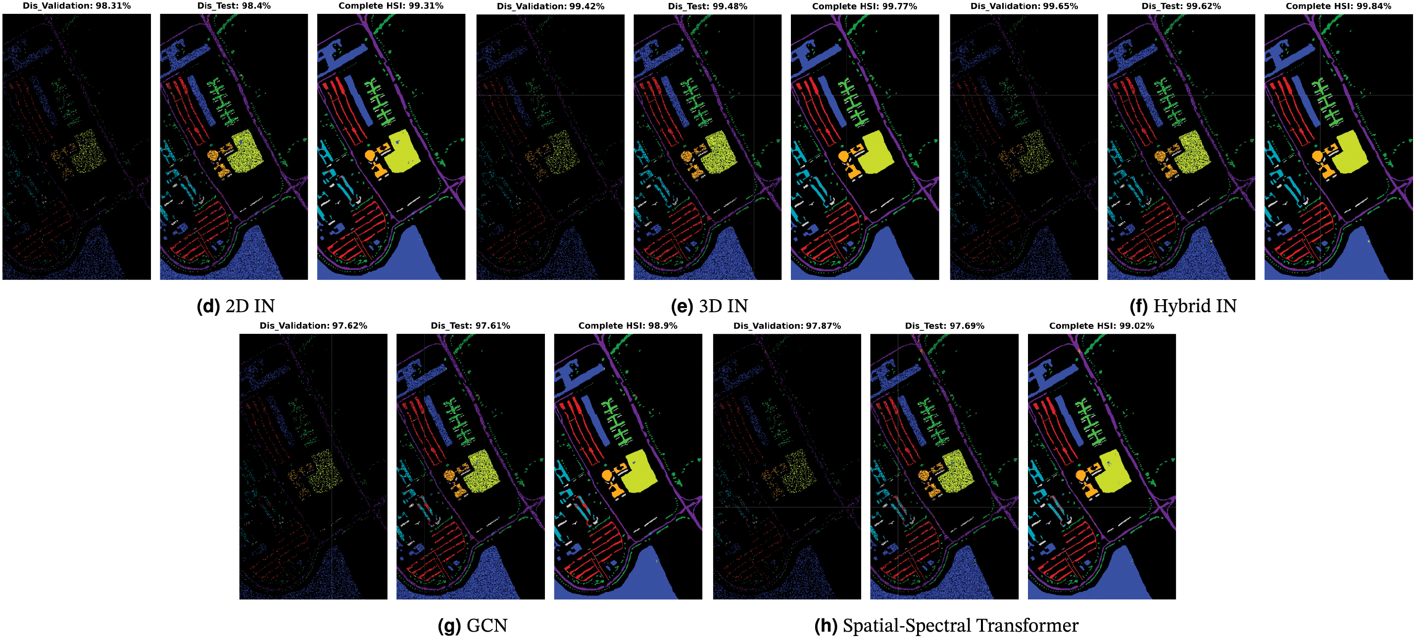
Figure 9: Pavia University Dataset: Land cover maps for disjoint validation, test, and the entire HSI used as a test set are provided. Comprehensive class-wise results can be found in Table 7

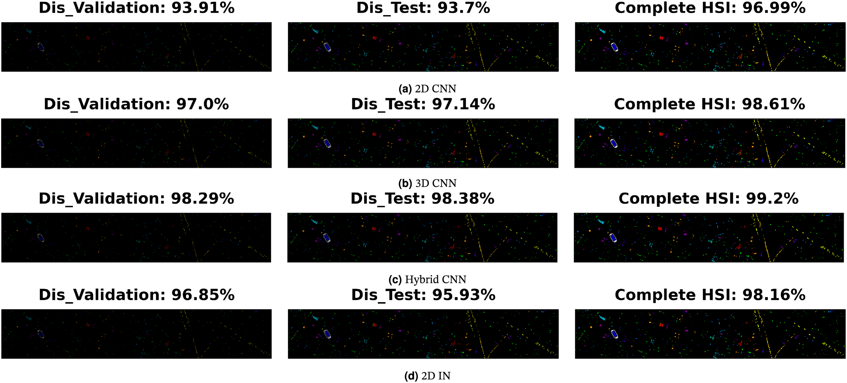
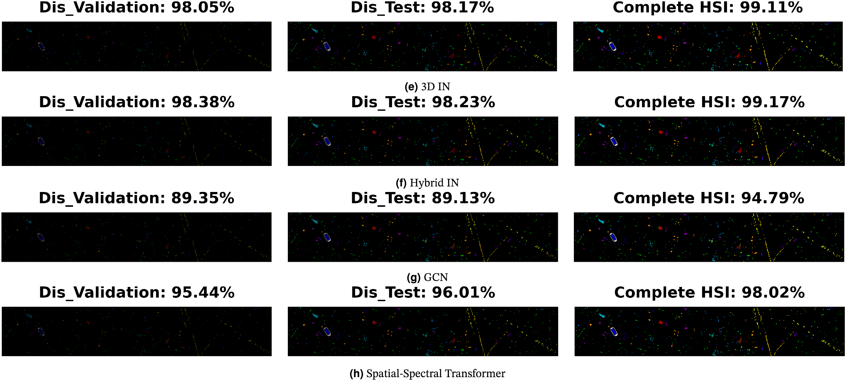
Figure 10: University Houston Dataset: Land cover maps for disjoint validation, test, and the entire HSI used as a test set are provided. Comprehensive class-wise results can be found in Table 8

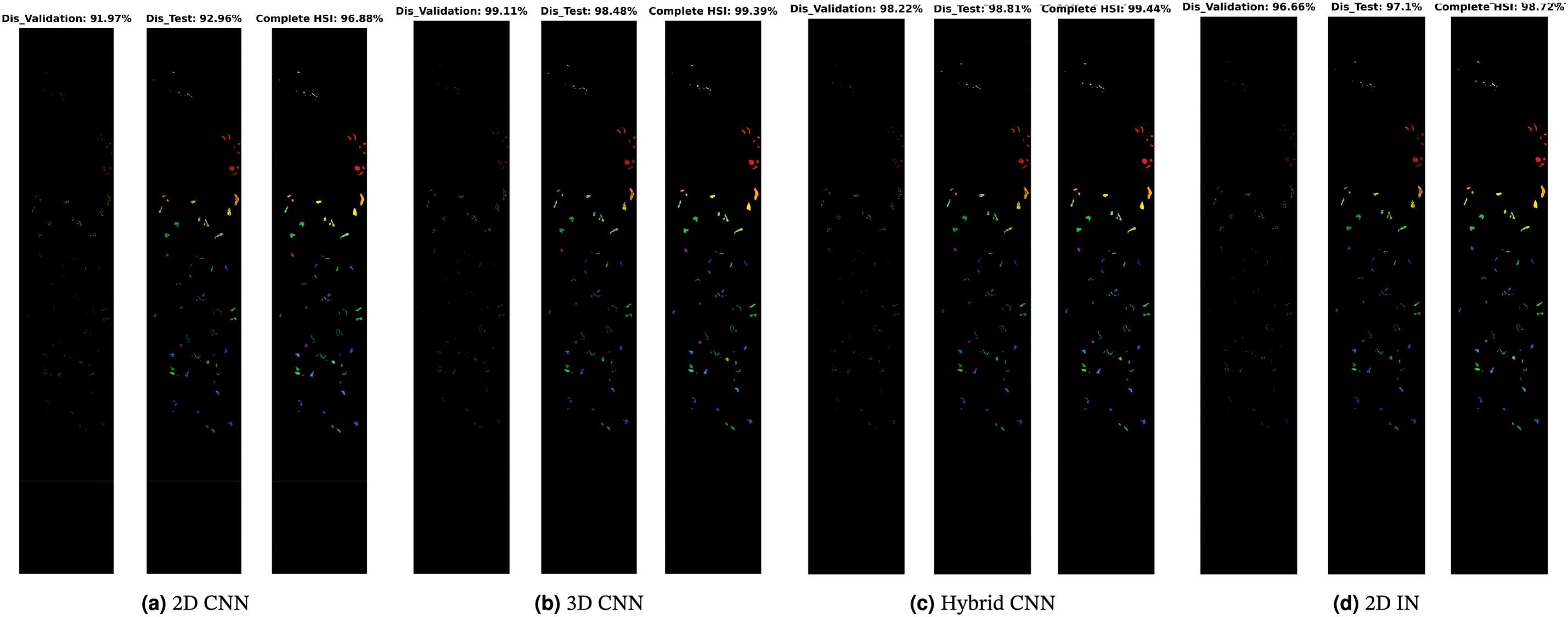
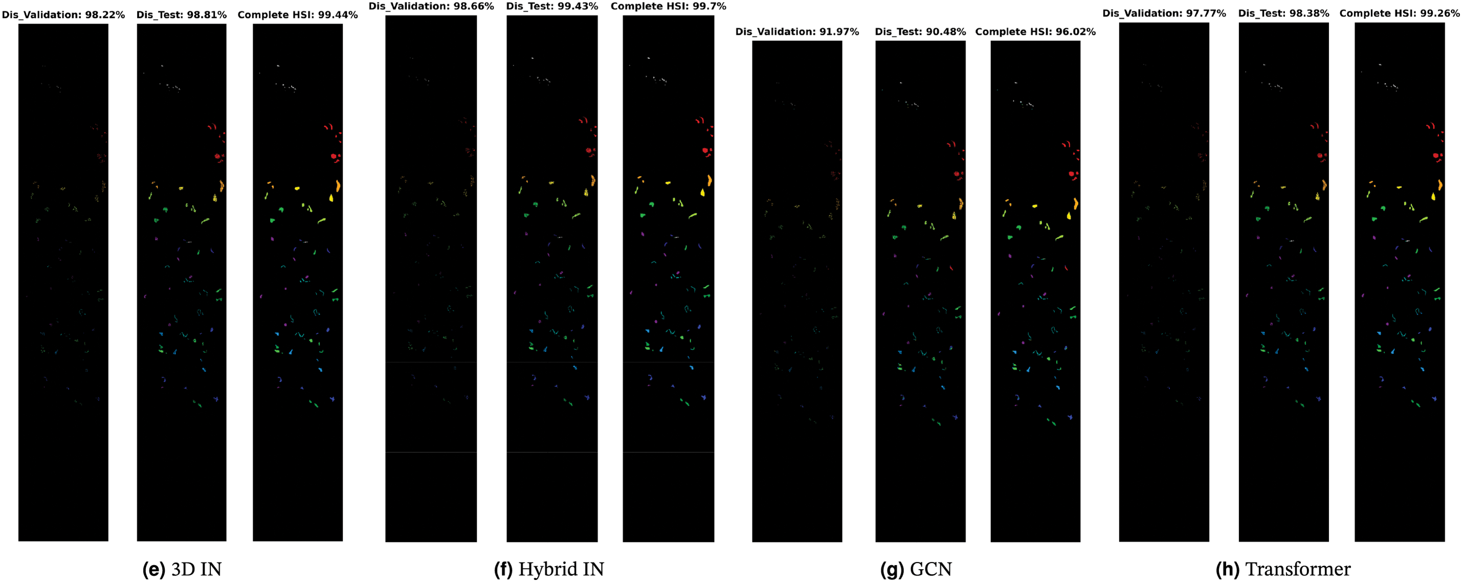
Figure 11: Botswana Dataset: Land cover maps for disjoint validation, test, and the entire HSI used as a test set are provided. Comprehensive class-wise results can be found in Table 9

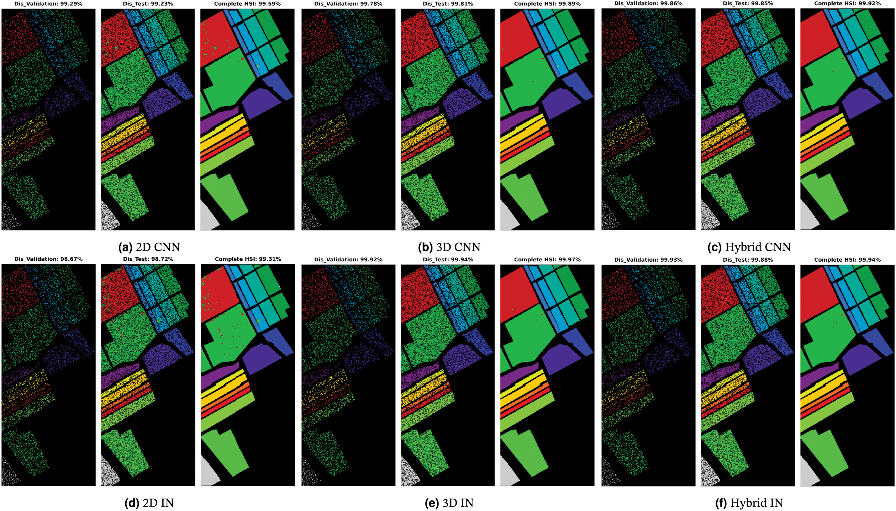
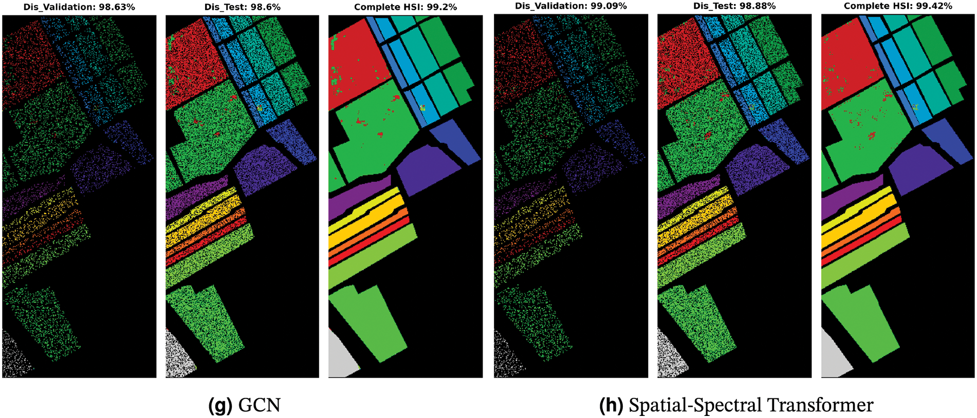
Figure 12: Salinas Dataset: Land cover maps for disjoint validation, test, and the entire HSI used as a test set are provided. Comprehensive class-wise results can be found in Table 10

The comparative methods frequently misclassify samples with similar spatial structures, exemplified by the misclassification of Meadows and Bare Soil classes in the Pavia University dataset, as illustrated in Fig. 9. Furthermore, the overall accuracy (OA) for the Grapes Untrained class is lower compared to other classes due to the aforementioned reasons as shown in Table 7. In summary, higher accuracy can be attained by employing a higher number of labeled samples (complete HSI dataset as the test set), as depicted in Figs. 8–12 and Tables 6–10, nevertheless, the elevated accuracy is accompanied by the drawbacks of bias, redundancy, and diminished generalization performance. Tables 6–10 also illustrate the computational time required to process and evaluate the HSI datasets used in this study. As depicted in the Tables, the time exhibits a gradual increase with the growing number of samples, i.e., Disjoint validation, disjoint test, and complete HSI dataset as a test set.

4  Statistical Tests

Average, overall, and Kappa accuracy may not always be appropriate measures, especially when there are significant differences in the number of samples in each class within a dataset. To clarify this point, consider the following scenario. Suppose we have a dataset with 90 healthy (positive) individuals and 10 not-healthy (negative) individuals. If a conventional model correctly predicts 90% of individuals as healthy, it might still predict the not-healthy individuals as healthy. What would be the best accuracy in this scenario?

In this setting, the model identifies 10 individuals as “False Negative”, 0 as “True Positive”, 0 as “False Positive”, and 90 as “True Negative”. Thus, the average accuracy would be 90%, i.e., 90+0100=0.9. However, the model is highly biased since it predicts all the not-healthy individuals as healthy. In such scenarios, overall and average accuracies can be misleading or misinterpreted, indicating that these measures alone are not sufficient for evaluating a machine learning model. Therefore, it is important to consider additional statistical measures to validate the model beyond simple accuracy metrics.

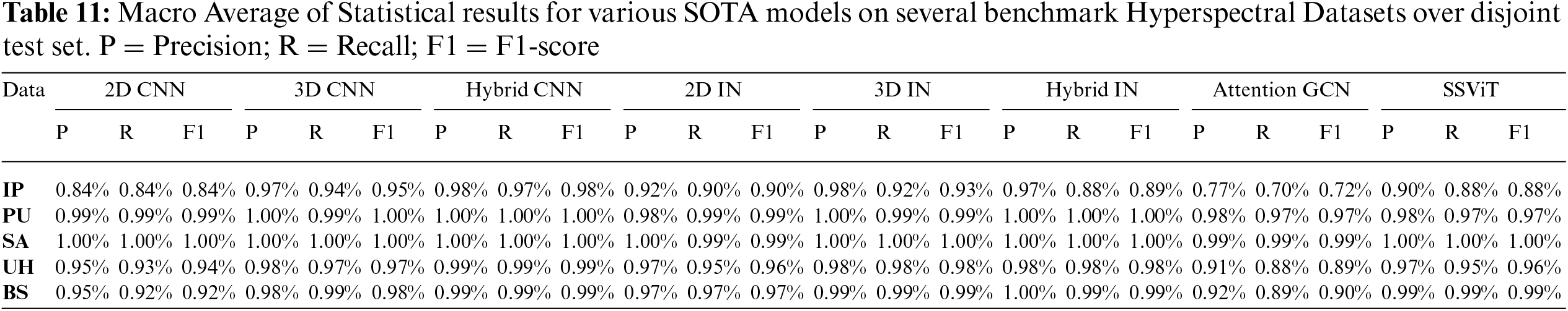
Several statistical tests can be used to validate the results. For this work, we consider Recall (True Positive Rate or Sensitivity), Precision (Positive Predictive Value, PPV), and F1 score (a harmonic mean of precision and recall). In an ideal scenario, PPV should be 1, which occurs when the numerator and denominator are equal, i.e., when True Positive (TP) equals TP + False Positive (FP), making FP equal to 0. As FP increases, PPV decreases, leading to an inappropriate model. A similar trend can be observed for Recall, where False Negative (FN) replaces FP. Recall and PPV can be computed as follows:

Recall=TPTP+FN(13)

Precision=TPTP+FP(14)

For a classification model to be effective, both Precision (Positive Predictive Value, PPV) and Recall need to be high, which means that both False Positives (FP) and False Negatives (FN) must be low. In addition to Recall and PPV, the F1 score should also be computed, as it combines both Recall and PPV to provide a single metric that offers statistical significance and deeper insight into the classifier’s generalization performance. The F1 score can be calculated as follows:

F1 score=2×Precision×RecallPrecision+Recall(15)

A model is considered effective if it achieves high values for PPV, Recall, and the F1 score. These metrics provide a more comprehensive evaluation of the model’s performance compared to using accuracy alone. The detailed statistical results are presented in Table 11.

5  Conclusion

This paper introduced a novel technique for generating disjoint train, validation, and test splits in Hyperspectral Image Classification (HSIC). By efficiently partitioning the ground truth data, the proposed technique ensured unbiased performance evaluations and facilitated reliable comparisons between classification models. It proved to be a valuable tool for creating disjoint splits, guaranteeing that the subsets were representative of the entire dataset and that the classification results were not skewed by data leakage. While the technique demonstrated significant advantages, limitations were acknowledged, and opportunities for further improvement were identified. Future research could investigate alternative data-splitting strategies that incorporate additional factors, such as class imbalance or spatial coherence, to further enhance the representativeness and generalizability of the subsets. Addressing these aspects could lead to the development of even more robust and effective data-splitting techniques for HSIC.

Acknowledgement: Not applicable.

Funding Statement: The authors extend their appreciation to the Researchers Supporting Project number (RSPD2024R848), King Saud University, Riyadh, Saudi Arabia.

Author Contributions: Study conception and desing: Muhammad Ahmad, Manuel Mazzara, Salvatore Distefano; Analysis and interpretation of results: Muhammad Ahmad, Hamad Ahmed Altuwaijri, Adil Mehmood Khan; manuscript preparation: Muhammad Ahmad, Manuel Mazzara, Salvatore Distefano, Adil Mehmood Khan, Hamad Ahmed Altuwaijri. All authors reviewed the results and approved the final version of the manuscript.

Availability of Data and Materials: The data used in this study is publicly available and can be accessed from the corresponding data repository https://www.ehu.eus/ccwintco/index.php/Hyperspectral_Remote_Sensing_Scenes (accessed on 2 January 2024). The source code for the experiments conducted in this paper can be accessed at https://github.com/mahmad00/Disjoint-Sampling-for-Hyperspectral-Image-Classification (accessed on 2 May 2024).

Ethics Approval: Not applicable.

Conflicts of Interest: The authors declare that they have no conflicts of interest to report regarding the present study.

References

1. M. Ahmad et al., “Hyperspectral image classification-traditional to deep models: A survey for future prospects,” IEEE J. Sel. Top. Appl. Earth Obs. Remote Sens., vol. 15, pp. 968–999, 2022. doi: 10.1109/JSTARS.2021.3133021. [Google Scholar] [CrossRef]

2. S. Aksoy, E. Sertel, R. Roscher, A. Tanik, and N. Hamzehpour, “Assessment of soil salinity using explainable machine learning methods and landsat 8 images,” Int. J. Appl. Earth Obs. Geoinf., vol. 130, 2024, Art. no. 103879. doi: 10.1016/j.jag.2024.103879. [Google Scholar] [CrossRef]

3. V. Lodhi, D. Chakravarty, and P. Mitra, “Hyperspectral imaging for earth observation: Platforms and instruments,” J. Indian Inst. Sci., vol. 98, no. 4, pp. 429–443, 2018. doi: 10.1007/s41745-018-0070-8. [Google Scholar] [CrossRef]

4. Y. Li, D. Hong, C. Li, J. Yao, and J. Chanussote, “HD-Net: High-resolution decoupled network for building footprint extraction via deeply supervised body and boundary decomposition,” ISPRS J. Photogramm. Remote Sens., vol. 209, no. 1, pp. 51–65, 2024. doi: 10.1016/j.isprsjprs.2024.01.022. [Google Scholar] [CrossRef]

5. T. Jiang, H. van der Werff, F. van Ruitenbeek, A. Dijkstra, C. Lievens and M. van der Meijde, “The influence of changing moisture content on laboratory acquired spectral feature parameters and mineral classification,” Int. J. Appl. Earth Obs. Geoinf., vol. 130, 2024, Art. no. 103884. doi: 10.1016/j.jag.2024.103884. [Google Scholar] [CrossRef]

6. B. Lu, P. D. Dao, J. Liu, Y. He, and J. Shang, “Recent advances of hyperspectral imaging technology and applications in agriculture,” Remote Sens., vol. 12, no. 16, 2020, Art. no. 2659. doi: 10.3390/rs12162659. [Google Scholar] [CrossRef]

7. T. Adão et al., “Hyperspectral imaging: A review on UAV-based sensors, data processing and applications for agriculture and forestry,” Remote Sens., vol. 9, no. 11, 2017, Art. no. 1110. doi: 10.3390/rs9111110. [Google Scholar] [CrossRef]

8. S. Chen et al., “CDasXORNet: Change detection of buildings from bi-temporal remote sensing images as an XOR problem,” Int. J. Appl. Earth Obs. Geoinf., vol. 130, no. 1, 2024, Art. no. 103836. doi: 10.1016/j.jag.2024.103836. [Google Scholar] [CrossRef]

9. C. Li, B. Zhang, D. Hong, J. Yao, and J. Chanussot, “LRR-Net: An interpretable deep unfolding network for hyperspectral anomaly detection,” IEEE Trans. Geosci. Remote Sens., vol. 61, pp. 1–12, 2023. doi: 10.1109/TGRS.2023.3279834. [Google Scholar] [CrossRef]

10. E. Bedini, “The use of hyperspectral remote sensing for mineral exploration: A review,” J. Hyperspectr. Remote Sens., vol. 7, no. 4, pp. 189–211, 2017. doi: 10.29150/jhrs.v7.4.p189-211. [Google Scholar] [CrossRef]

11. C. Weber et al., “Hyperspectral imagery for environmental urban planning,” in IGARSS 2018—2018 IEEE Int. Geosci. Remote Sens. Symp., IEEE, 2018, pp. 1628–1631. [Google Scholar]

12. M. B. Stuart, A. J. McGonigle, and J. R. Willmott, “Hyperspectral imaging in environmental monitoring: A review of recent developments and technological advances in compact field deployable systems,” Sensors, vol. 19, no. 14, 2019, Art. no. 3071. doi: 10.3390/s19143071. [Google Scholar] [PubMed] [CrossRef]

13. C. B. Pande and K. N. Moharir, “Application of hyperspectral remote sensing role in precision farming and sustainable agriculture under climate change: A review,” in Climate Change Impacts on Natural Resources, Ecosystems and Agricultural Systems, Springer International Publishing, 2023, pp. 503–520. doi: 10.1007/978-3-031-19059-9_21. [Google Scholar] [CrossRef]

14. S. Wang, W. Han, X. Huang, X. Zhang, L. Wang, and J. Li, “Trustworthy remote sensing interpretation: Concepts, technologies, and applications,” ISPRS J. Photogramm. Remote Sens., vol. 209, no. 3, pp. 150–172, 2024. doi: 10.1016/j.isprsjprs.2024.02.003. [Google Scholar] [CrossRef]

15. S. S. Deshpande and A. B. Inamdar, Hyperspectral Remote Sensing in Urban Environments. UK: Routledge Taylor & Francis Group, 2023. [Google Scholar]

16. P. Sajadi et al., “Automated pixel purification for delineating pervious and impervious surfaces in a city using advanced hyperspectral imagery techniques,” IEEE Access, vol. 12, no. 1, pp. 82560–82583, 2024. doi: 10.1109/ACCESS.2024.3408805. [Google Scholar] [CrossRef]

17. A. Chauhan et al., “Chapter 10-earth observation applications for urban mapping and monitoring: Research prospects, opportunities and challenges,” in Earth Observation in Urban Monitoring, Earth Observation, A. Kumar, P. K. Srivastava, P. Saikia, R. K. Mall, Eds., Elsevier, 2024, pp. 197–229. [Google Scholar]

18. D. Hong et al., “SpectralGPT: Spectral remote sensing foundation model,” IEEE Trans. Pattern Anal. Mach. Intell., vol. 46, no. 8, pp. 5227–5244, 2024. doi: 10.1109/TPAMI.2024.3362475. [Google Scholar] [PubMed] [CrossRef]

19. I. Ahmad, G. Farooque, Q. Liu, F. Hadi, and L. Xiao, “MSTSENet: Multiscale spectral-spatial transformer with squeeze and excitation network for hyperspectral image classification,” Eng. Appl. Artif. Intell., vol. 134, no. 3, 2024, Art. no. 108669. doi: 10.1016/j.engappai.2024.108669. [Google Scholar] [CrossRef]

20. M. Ahmad, A. M. Khan, M. Mazzara, S. Distefano, M. Ali and M. S. Sarfraz, “A fast and compact 3-D CNN for hyperspectral image classification,” IEEE Geosci. Remote Sens. Lett., vol. 19, pp. 1–5, 2022. doi: 10.1109/LGRS.2020.3043710. [Google Scholar] [CrossRef]

21. D. Hong, L. Gao, J. Yao, B. Zhang, A. Plaza and J. Chanussot, “Graph convolutional networks for hyperspectral image classification,” IEEE Trans. Geosci. Remote Sens., vol. 59, no. 7, pp. 5966–5978, 2021. doi: 10.1109/TGRS.2020.3015157. [Google Scholar] [CrossRef]

22. A. Jamali, S. K. Roy, D. Hong, P. M. Atkinson, and P. Ghamisi, “Attention graph convolutional network for disjoint hyperspectral image classification,” IEEE Geosci. Remote Sens. Lett., 2024. doi: 10.1109/LGRS.2024.3356422. [Google Scholar] [CrossRef]

23. J. Yao, B. Zhang, C. Li, D. Hong, and J. Chanussot, “Extended vision transformer (ExViT) for land use and land cover classification: A multimodal deep learning framework,” IEEE Trans. Geosci. Remote Sens., vol. 61, pp. 1–15, 2023. doi: 10.1109/TGRS.2023.3284671. [Google Scholar] [CrossRef]

24. M. Ahmad, U. Ghous, M. Usama, and M. Mazzara, “Waveformer: Spectral-spatial wavelet transformer for hyperspectral image classification,” IEEE Geosci. Remote Sens. Lett., vol. 21, pp. 1–5, 2024. doi: 10.1109/LGRS.2024.3441938. [Google Scholar] [CrossRef]

25. M. Ahmad and M. Mazzara, “SCSNet: Sharpened cosine similarity-based neural network for hyperspectral image classification,” IEEE Geosci. Remote Sens. Lett., vol. 21, pp. 1–4, 2024. doi: 10.1109/LGRS.2024.3365611. [Google Scholar] [CrossRef]

26. T. Lu, Y. Fang, W. Fu, K. Ding, and X. Kang, “Dual-stream class-adaptive network for semi-supervised hyperspectral image classification,” IEEE Trans. Geosci. Remote Sens., vol. 62, pp. 1–11, 2024. doi: 10.1109/TGRS.2024.3357455. [Google Scholar] [CrossRef]

27. M. Ahmad, M. Usama, A. M. Khan, S. Distefano, H. A. Altuwaijri and M. Mazzara, “Spatial spectral transformer with conditional position encoding for hyperspectral image classification,” IEEE Geosci. Remote Sens. Lett., vol. 21, 2024, Art. no. 5508205. doi: 10.1109/LGRS.2024.3431188. [Google Scholar] [CrossRef]

28. H. Tan et al., “Data pruning via moving-one-sample-out,” in Advances in Neural Information Processing Systems, A. Oh, T. Naumann, A. Globerson, K. Saenko, M. Hardt, S. Levine, Eds., Curran Associates, Inc., 2023, vol. 36. [Google Scholar]

29. M. Ahmad et al., “A disjoint samples-based 3D-CNN with active transfer learning for hyperspectral image classification,” IEEE Trans. Geosci. Remote Sens., vol. 60, pp. 1–16, 2022. doi: 10.1109/TGRS.2022.3209182. [Google Scholar] [CrossRef]

30. C. Geiß, P. Aravena Pelizar, H. Schrade, A. Brenning, and H. Taubenböck, “On the effect of spatially non-disjoint training and test samples on estimated model generalization capabilities in supervised classification with spatial features,” IEEE Geosci. Remote Sens. Lett., vol. 14, no. 11, pp. 2008–2012, 2017. doi: 10.1109/LGRS.2017.2747222. [Google Scholar] [CrossRef]

31. M. Ahmad et al., “Spatial prior fuzziness pool-based interactive classification of hyperspectral images,” Remote Sens., vol. 11, no. 9, 2019, Art. no. 1136. doi: 10.3390/rs11091136. [Google Scholar] [CrossRef]

32. P. Zhang, H. Yu, P. Li, and R. Wang, “TransHSI: A hybrid CNN-transformer method for disjoint sample-based hyperspectral image classification,” Remote Sens., vol. 15, no. 22, 2023. doi: 10.3390/rs15225331. [Google Scholar] [CrossRef]

33. D. Hong, C. Li, B. Zhang, N. Yokoya, J. A. Benediktsson and J. Chanussot, “Multimodal artificial intelligence foundation models: Unleashing the power of remote sensing big data in earth observation,” Innov. Geosci., vol. 2, no. 1, 2024, Art. no. 100055. doi: 10.59717/j.xinn-geo.2024.100055. [Google Scholar] [CrossRef]

34. J. Yao, D. Hong, H. Wang, H. Liu, and J. Chanussot, “UCSL: Toward unsupervised common subspace learning for cross-modal image classification,” IEEE Trans. Geosci. Remote Sens., vol. 61, pp. 1–12, 2023. doi: 10.1109/TGRS.2023.3282951. [Google Scholar] [CrossRef]

35. J. Yao, D. Hong, C. Li, and J. Chanussot, “SpectralMamba: Efficient mamba for hyperspectral image classification,” 2024, arXiv:2404.08489. [Google Scholar]

36. D. Hong et al., “Cross-city matters: A multimodal remote sensing benchmark dataset for cross-city semantic segmentation using high-resolution domain adaptation networks,” Remote Sens. Environ., vol. 299, 2023, Art. no. 113856. doi: 10.1016/j.rse.2023.113856. [Google Scholar] [CrossRef]

37. J. Yao et al., “Semi-active convolutional neural networks for hyperspectral image classification,” IEEE Trans. Geosci. Remote Sens., vol. 60, no. 2, pp. 1–15, 2022. doi: 10.1109/TGRS.2022.3230411. [Google Scholar] [CrossRef]

38. U. Ghous, M. S. Sarfraz, M. Ahmad, C. Li, and D. Hong, “(2+1)D extreme xception net for hyperspectral image classification,” IEEE J. Sel. Top. Appl. Earth Obs. Remote Sens., vol. 17, pp. 5159–5172, 2024. doi: 10.1109/JSTARS.2024.3362936. [Google Scholar] [CrossRef]

39. S. K. Adari and S. Alla, “Introduction to machine learning,” in Beginning Anomaly Detection Using Python-Based Deep Learning: Implement Anomaly Detection Applications with Keras and PyTorch. Berkeley, CA: Apress, 2024, pp. 105–134. [Google Scholar]

40. S. K. Roy, G. Krishna, S. R. Dubey, and B. B. Chaudhuri, “HybridSN: Exploring 3-D-2-D CNN feature hierarchy for hyperspectral image classification,” IEEE Geosci. Remote Sens. Lett., vol. 17, no. 2, pp. 277–281, 2020. doi: 10.1109/LGRS.2019.2918719. [Google Scholar] [CrossRef]

41. Y. Wang, X. Yu, X. Wen, X. Li, H. Dong and S. Zang, “Learning a 3-D-CNN and convolution transformers for hyperspectral image classification,” IEEE Geosci. Remote Sens. Lett., vol. 21, pp. 1–5, 2024. doi: 10.1109/LGRS.2024.3365615. [Google Scholar] [CrossRef]

42. L. Song, Z. Feng, S. Yang, X. Zhang, and L. Jiao, “Interactive spectral-spatial transformer for hyperspectral image classification,” IEEE Trans. Circuits Syst. Video Technol., 2024. doi: 10.1109/TCSVT.2024.3386578. [Google Scholar] [CrossRef]

43. X. Yang et al., “Synergistic 2D/3D convolutional neural network for hyperspectral image classification,” Remote Sens., vol. 12, no. 12, 2020, Art. no. 2033. doi: 10.3390/rs12122033. [Google Scholar] [CrossRef]

44. W. Liao, F. Wang, and H. Zhao, “Hyperspectral image classification using attention-only spatial-spectral network based on transformer,” IEEE Access, vol. 12, pp. 93677–93688, 2024. doi: 10.1109/ACCESS.2024.3424674. [Google Scholar] [CrossRef]

45. T. Arshad and J. Zhang, “A light-weighted spectral-spatial transformer model for hyperspectral image classification,” IEEE J. Sel. Top. Appl. Earth Obs. Remote Sens., vol. 17, pp. 12008–12019, 2024. doi: 10.1109/JSTARS.2024.3419070. [Google Scholar] [CrossRef]

46. R. Khan, T. Arshad, X. Ma, W. Chen, H. F. Zhu and Y. N. Wu, “Deep spectral spatial feature enhancement through transformer for hyperspectral image classification,” IEEE Geosci. Remote Sens. Lett., vol. 21, pp. 1–5, 2024. doi: 10.1109/LGRS.2024.3424986. [Google Scholar] [CrossRef]

47. H. Fırat, M. E. Asker, M. I. Bayındır, and D. Hanbay, “Hybrid 3D/2D complete inception module and convolutional neural network for hyperspectral remote sensing image classification,” Neural Process. Lett., vol. 55, no. 2, pp. 1087–1130, 2023. doi: 10.1007/s11063-022-10929-z. [Google Scholar] [CrossRef]

48. X. Zhang, “Improved three-dimensional inception networks for hyperspectral remote sensing image classification,” IEEE Access, vol. 11, pp. 32648–32658, 2023. doi: 10.1109/ACCESS.2023.3262992. [Google Scholar] [CrossRef]

49. Z. Xiong, Y. Yuan, and Q. Wang, “AI-NET: Attention inception neural networks for hyperspectral image classification,” in IGARSS 2018—2018 IEEE Int. Geosci. Remote Sens. Symp., IEEE, 2018. [Google Scholar]

50. X. Wu, D. Hong, and J. Chanussot, “Convolutional neural networks for multimodal remote sensing data classification,” IEEE Trans. Geosci. Remote Sens., vol. 60, pp. 1–10, 2022. doi: 10.1109/TGRS.2022.3228927. [Google Scholar] [CrossRef]

51. S. Ghaderizadeh, D. Abbasi-Moghadam, A. Sharifi, N. Zhao, and A. Tariq, “Hyperspectral image classification using a hybrid 3D-2D convolutional neural networks,” IEEE J. Sel. Top. Appl. Earth Obs. Remote Sens., vol. 14, pp. 7570–7588, 2021. doi: 10.1109/JSTARS.2021.3099118. [Google Scholar] [CrossRef]

52. X. Yang, Y. Ye, X. Li, R. Y. Lau, X. Zhang and X. Huang, “Hyperspectral image classification with deep learning models,” IEEE Trans. Geosci. Remote Sens., vol. 56, no. 9, pp. 5408–5423, 2018. doi: 10.1109/TGRS.2018.2815613. [Google Scholar] [CrossRef]