Short-Term Wind Power Prediction Based on WVMD and Spatio-Temporal Dual-Stream Network

1  Introduction

Due to its low cost, abundance, and environmental friendliness, wind energy has gained global attention [1,2]. However, the inherent volatility, intermittence, and uncertainty of wind power pose significant challenges to the safe and stable operation of power systems. Therefore, accurate wind power prediction is crucial for improving the reliability and safety of system operations [3].

Currently, wind power prediction methods are mainly divided into four categories: physical methods, statistical methods, traditional machine learning methods and deep learning methods. Although the first three traditional ones have certain applications in wind power prediction, there are also some limitations and challenges. The physical method has high requirements on the accuracy of meteorological factors, and it is difficult to cope with the complex and changeable wind field conditions [4]. The statistical method lacks the ability to model nonlinear relationships and has poor adaptability to complex wind farm dynamic changes [5]. Traditional machine learning performs poorly on nonlinear and non-stationary data and has limited model generalization ability [6]. In contrast, deep learning technology has great advantages and has become the current mainstream method [7].

In wind power prediction using deep learning, initial approaches employed single models such as LSTM [8], CNN [9,10], GRU [11], and BiGRU [12]. However, wind power data consist of sequential information that includes both temporal and spatial components [13]. While single models effectively handle temporal data from time series of wind power, they often overlook spatial features. Spatial information in this context encompasses different geographical locations [14] and diverse meteorological factors [15]. To address these spatio-temporal characteristics, hybrid models have been developed for wind power prediction using deep learning techniques. These include CNN-LSTM [16], CNN-BiLSTM [17], CNN-BiLSTM-AM [18], etc. Although the above hybrid models can effectively deal with spatio-temporal features, they also increase the complexity. The two-stream network applied to action recognition [19] presented recently, uses parallel processing to handle spatio-temporal features and shows superior performance than the hybrid models. Therefore, it is applied to some fields rapidly. For example, Reference [20] proposes a two-stream three-dimensional CNN, which captures spatial and temporal information on a fine time scale for skeletal-based action recognition. Reference [21] proposes a DSN composed of CNN and GRU to learn spatio-temporal features from photovoltaic power generation and meteorological data, which improved the accuracy of prediction. Thus, it is natural to adopt it in the field of wind power prediction. However, how to improve the construction of DSN is still a challenge. Generally, one branch of the DSN processes spatial data while the other handles temporal data. What types of networks are used for each branch, and how many are there? The features generated by these branches may have some redundancy. How can this redundancy be reduced? These are some of the challenges faced in this field.

Additionally, to address the intermittency, volatility, and uncertainty of wind power generation, the aforementioned models often incorporate data preprocessing methods such as empirical mode decomposition (EMD) [22], ensemble empirical mode decomposition (EEMD) [23], wavelet transform (WT) [24], and variational mode decomposition (VMD) [25]. Among them, the VMD technology shows the best performance and noise robustness [16,25]. However, one of the drawbacks of this method is that the number of mode components K and penalty factor a have a large impact on the decomposition results [26]. Hence, it is important to consider the optimal combination of key parameters K and a of VMD.

Motivated by the basic ideas mentioned above, the paper proposes a superior wind power named WVMD-DSN. It first utilizes the PCC to choose some NWP features to form the feature set, Then, it decomposes the feature set using VMD, while adopting WOA to fine-tune the number of mode components K and penalty factor a. Finally, it constructs the DSN for short-term wind power prediction, integrating AM, SENet, and BiGRU.

The main contributions of this paper are as follows:

1)   It proposes a novel dual-stream network model and applies it to wind power generation, achieving better prediction results than other baseline models and demonstrating strong generalization performance.

2)   In order to enhance the prediction accuracy and address potential errors, it introduces WOA to design the key parameters of VMD adaptively.

2  Background Technologies

In this chapter, we first discuss the theoretical foundation of VMD preprocessing technology and the evaluation indices of envelope entropy and mutual information used for WOA-optimized VMD. We then explain the theoretical underpinnings of SENet and BiGRU as employed in the DSN network model.

2.1 VMD and WOA

VMD is an adaptive signal decomposition method that employs a non-recursive decomposition scheme [27]. It decomposes signals into a specified number of IMFs with different center frequencies. Applying the VMD decomposition preprocessing method to wind power involves the following constrained variational model:

min|uk|.|ωk|⁡{∑k=1K‖∂t[(δ(t)+jπt)∗uk(t)]e−jwkt‖22s.t.∑k=1Kuk(t)=X~(t)(1)

In the equation, X~(t) is the wind power generation series; K is the number of modes to be decomposed; δ(t) is the Dirac function; j is the imaginary unit; t is time; uk(t) is the IMF component at time k; ωk is the central frequency corresponding to the IMF component; ∗ is convolution operation.

To solve Eq. (1), the Lagrange multiplication operator λ is introduced to transform the constrained problem into a non-constrained problem and obtain the augmented Lagrange expression.

L(uk, ωk, λ)=α∑k=1K‖∂t[(δ(t)+jπt)∗uk(t)]e−jωkt‖22+‖f(t)−∑k=1Kuk(t)‖22+⟨λ(t), f(t)−∑k=1Kuk(t)⟩(2)

In Eq. (2), α is the penalty factor, which is used to reduce the influence of Gaussian noise. The parameters uk, ωk and λ are iteratively updated by the alternate direction method of the multiplier.

WOA [28] is a swarm intelligence optimization algorithm that effectively prevents getting trapped in local minima, unlike Particle Swarm Optimization (PSO) [29] and Grey Wolf Optimizer (GWO) [30], thereby enhancing global optimization efficiency. Therefore, it is suitable to solve some complex, changeable and nonlinear problems. Mutual Information (MI) primarily used in information theory to quantify the degree of correlation between two events, is less susceptible to external interference [31]. Here, we adopt WOA to optimize the key parameters K and α of VMD, and choose the envelope entropy and MI as the fitness function. The size of the envelope entropy reflects the uncertainty of the probability distribution. The larger the entropy, the greater the uncertainty of the signal. The calculation of the envelope entropy Ep of signal X~(t) is as follows:

{Ep=−∑t=1Nptlg⁡ptpt=a(t)∑t=1Na(t)(3)

Whereas, N is the number of sampled points of the signal, a(t) is the envelope signal obtained through Hilbert demodulation of signal X~(t), and pt represents the normalized result of signal a(t).

MI expression is as follows:

MI(X, Y)=H(Y)−H(Y|X)(4)

In the equation, X and Y represent different events, H(X) is the entropy of Y, H(Y|X) is the conditional entropy of Y given X. The normalized mutual information is processed as follows:

mi=MI(X, Y)/H(X)⋅H(Y)(5)

A higher mutual information entropy value indicates a stronger correlation between two events. For IMF components, those that better capture the characteristic information of the wind power signal will have a larger mutual information entropy value. The composite index established in this article is:

I=Ep∗mi(6)

The composite index considers both the noise level and characteristic information of IMF components. When an IMF component contains less noise and richer characteristic information, the composite index I has a smaller value. Therefore, the minimum value of I is adopted as the fitness function, expressed as:

fitness=min1∼K{I}(7)

2.2 SENet and BiGRU

SENet [32] is a CNN-based attention mechanism for learning feature relationships between different channels. By introducing the squeeze-excitation (SE) module, it learns the relationship between the CNN convolution kernel’s channels, and employs the channel AM to adaptively recalibrate channel-wise feature responses by explicitly modeling the interdependencies. SEblock adjusts the importance of each convolutional channel by learning their weights, thereby enhancing the network’s perception of different feature channels. The formula is as follows:

zc=1h×w∑1≤i≤h1≤j≤wuc(i, j)(8)

s=σ(w2δ(w1z))(9)

x~c=sc⋅uc(10)

In Eq. (8), zc is the squeeze output, and uc is the eigenvalue of the characteristic graph in channel c. In Eq. (9), w2 and w1 are fully connected layer operation, and δ denotes a ReLU layer operation. And then the output go through the sigmoid function σ to get s which is to characterize the weights of feature maps in matrix uc. In Eq. (10), sc reflects the importance weight of each feature channel, and the weight coefficient of each channel can be learned through sc⋅uc.

As for BiGRU, it is on the base of the traditional GRU [33] network, which the transmission of information is unidirectional. The mathematical model is shown below:

rt=σ(Wr⋅[ht−1, xt]+br)(11)

zt=σ(Wz⋅[ht−1, xt]+bz)(12)

h~t=tanh⁡(Wh⋅[rt∗ht−1, xt]+bh)(13)

ht=(1−zt)∗ht−1+zt∗h~t(14)

In the equations, Wr, Wz and Wh are the weights of the internal parameters of the GRU. br, bz and bh are the biases of the internal parameters of the GRU. σ is the sigmoid function, and tanh is the hyperbolic tangent function.

In the wind power forecasting, the current output relates not only to the state at the subsequent time but also to the previous. The input information at each time step is fed into two GRU networks in opposite directions in a BiGRU. Therefore, the BiGRU model can capture the strong temporal correlations in wind power sequences effectively.

3  WVMD_DSN Model

The proposed WVMD_DSN is illustrated in Fig. 1, which primarily consists of the following steps:

(1)   Clean the data, and then split the data into NWP and wind power data.

(2)   Decompose the wind power by VMD and get the IMF components. Here VMD is optimized by WOA to select the best mode number K and penalty factor.

(3)   Using PCC to calculate the correlation between NWP data and power features, and choose those with stronger correlations to form the feature set NWPpcc.

(4)   Integrating the NWPpcc and IMF components to form the input sets.

(5)   Predict each value by DSN, which integrates SENet, BiGRU, and AM.

(6)   Combine all the predicted values to form the final value.

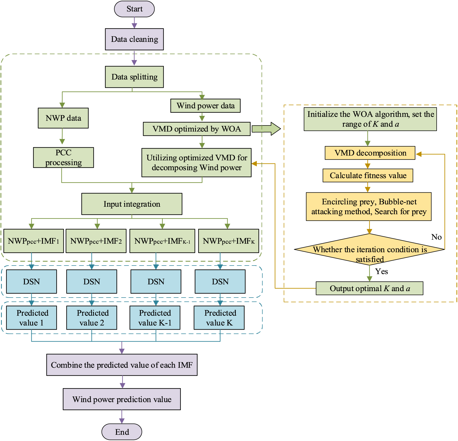
Figure 1: The architecture of WVMD_DSN

3.1 Data Preprocessing

The study utilizes spatio-temporal data consisting of Wind Power, Wind Speed-10 (WS-10), Wind Speed-30 (WS-30), Wind Speed-50 (WS-50), Wind Direction-10 (WD-10), Wind Direction-30 (WD-30), Wind Direction-50 (WD-50), Humidity, Temperature and Atmospheric Pressure. Here, Wind Speed-10 represents the wind speed at 10 m on the wind measurement tower, and the other numeric features follow the same meanings. The data preprocessing methods include the mean imputation for missing values and the MinMax scaling technique to normalize each attribute to the range of 0 to 1. Further, it employs PCC to select highly correlated NWP features. Additionally, to reduce the non-stationary characteristics of wind power, VMD is employed for decomposition, obtaining the IMF components. This is illustrated in Fig. 2, where K represents the number of IMFs.

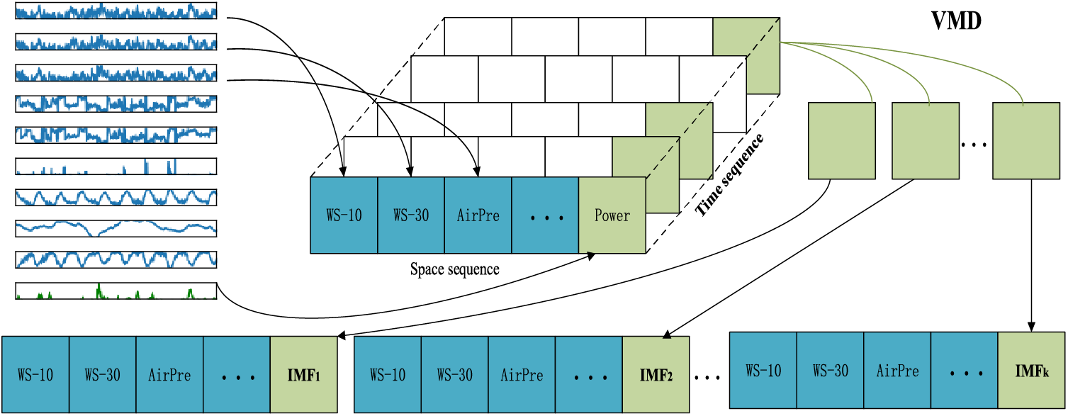
Figure 2: Schematic diagram of spatio-temporal wind power data processing based on VMD decomposition

After preprocessing the data, we employ a sliding window approach to select temporal data and prediction labels for the model. We use data from the first two hours as input, with a sample resolution of fifteen minutes. The sliding window size is set to 8, and the label window corresponds to the next fifteen minutes, with a prediction step of 1. Finally, the dataset is divided into training, validation, and test sets.

3.2 DSN Structure

In the paper, the proposed DSN consists of SENet and BiGRU, using for parallel processing of spatio-temporal features, as shown in Fig. 3. It extracts irregular trends and complex features from the variables of historical wind power data. The first stream uses SENet, which alone cannot capture spatio-temporal information. Therefore, we introduce a second stream using BiGRU. The SENet stream processes spatial data from NWP, including variables such as temperature, humidity, wind speed, and IMF components from VMD. The BiGRU stream focuses on extracting time series data of wind power also processed by VMD. The BiGRU stream mainly extracts the time series data of wind power processed by VMD.

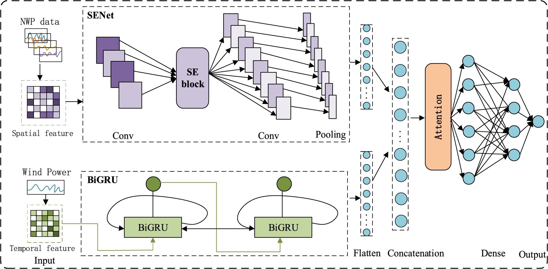
Figure 3: DSN network structure

The DSN includes an input layer, multiple hidden layers, and an output layer. The SENet stream’s hidden layers consist of convolutional layers, SEblocks, and pooling layers, which extract spatial features from various meteorological factors influencing wind power generation, that is the NWP data. The BiGRU stream comprises two BiGRU layers, which capture the temporal features of wind power generation. Then, the outputs of both streams are concatenated to form a single feature vector, which is passed to an attention module to extract more valuable output results. It produces the ultimately wind power prediction result.

4  Experiments and Results Analysis

In this chapter, we first describe the attributes of the two wind power datasets used in this paper. Next, we detail the WVMD preprocessing technique and the parameters employed in the DSN model. We then assess the efficacy of WVMD denoising by comparing the processed signals with Gaussian white noise and a normal distribution. Following this, WVMD is applied to wind power data. Finally, we perform ablation experiments to analyze the parallel computing time of the DSN model, compare WVMD_DSN with the current baseline model, and conduct a generalization analysis using wind power dataset 2. This comprehensive approach demonstrates the effectiveness of the WVMD_DSN method in wind power prediction.

4.1 Datasets

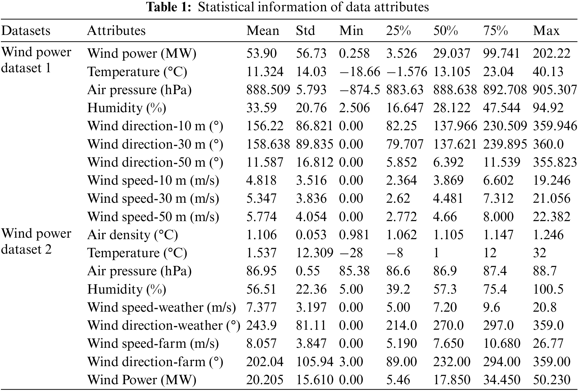
To evaluate the proposed WVMD_DSN, it uses the actual power and weather forecast numerical data collected from a region in Xinjiang, China. The data sampling period spans from 1 January, 2019 to December 31, 2019, with a sampling frequency of 15 min. Thus it consists in a total of 35,040 data points. Wind power generation dataset includes historical wind power and NWP data, that is, timestamp, Wind Power (WP), Temperature (Tem), Air Pressure (AP), Humidity (Hum), Wind Direction (WD), and Wind Speed (WS). To further investigate the generalization ability of the WVMD_DSN model, wind power dataset 2 is adopt. This dataset originated from Inner Mongolia, China. The specific features of wind power generation include timestamps, Air Density (AD), Temperature (Tem), Air Pressure (AP), Humidity (Hum), Wind Speed (WS), Wind Direction (WD), and Wind Power (WP). The sample information of the two datasets are shown in Table 1.

4.2 Experimental Parameter Settings

The experiments in this study are conducted using Python 3.7 and the TensorFlow framework. They are performed on a server equipped with an AMD Ryzen 9 5900HX CPU @ 4.6 GHz, an NVIDIA GeForce RTX 4090 GPU, and 24 GB of RAM.

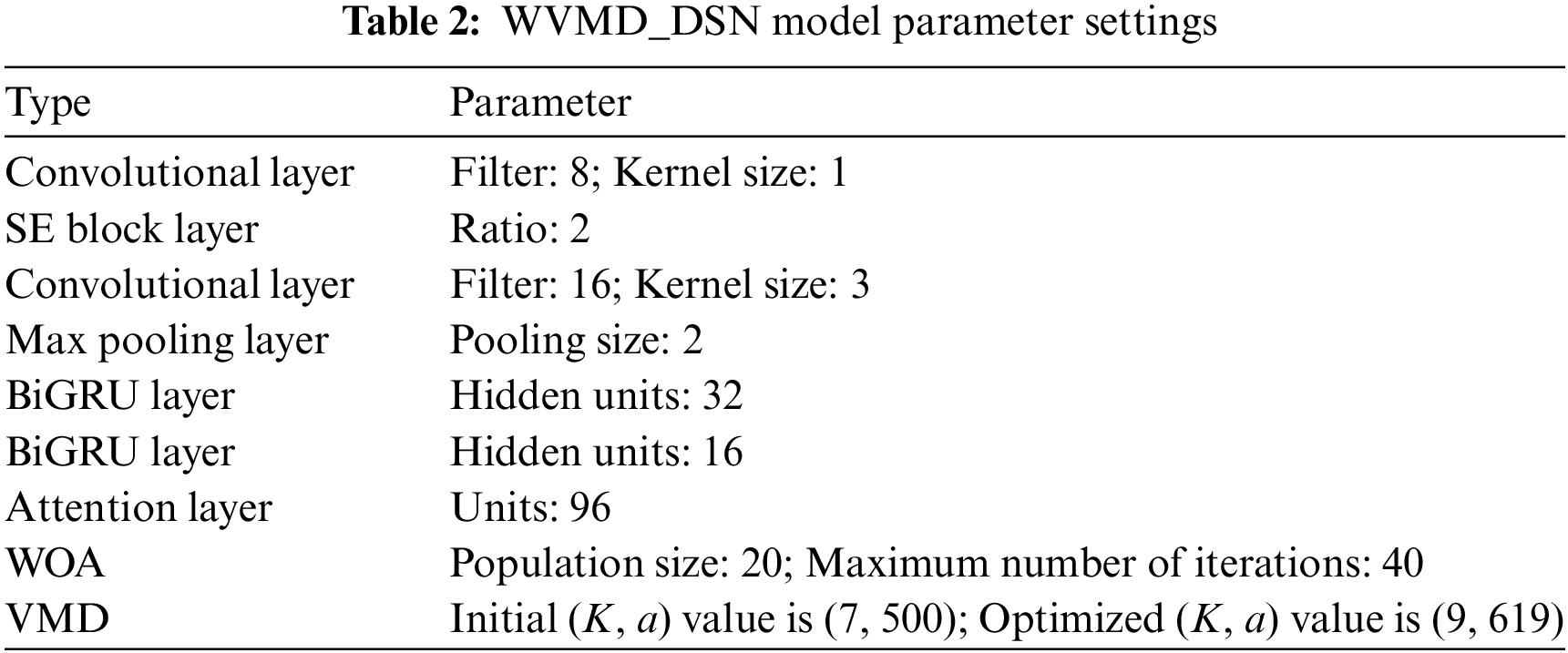
The WVMD_DSN model uses the Adam optimization algorithm with training epochs set to 100. Table 2 illustrates the parameter settings for the WOA optimization algorithm and the parameter settings for the DSN dual-stream network structure.

4.3 WVMD Processing

4.3.1 Analysis of WVMD Decomposition Techniques

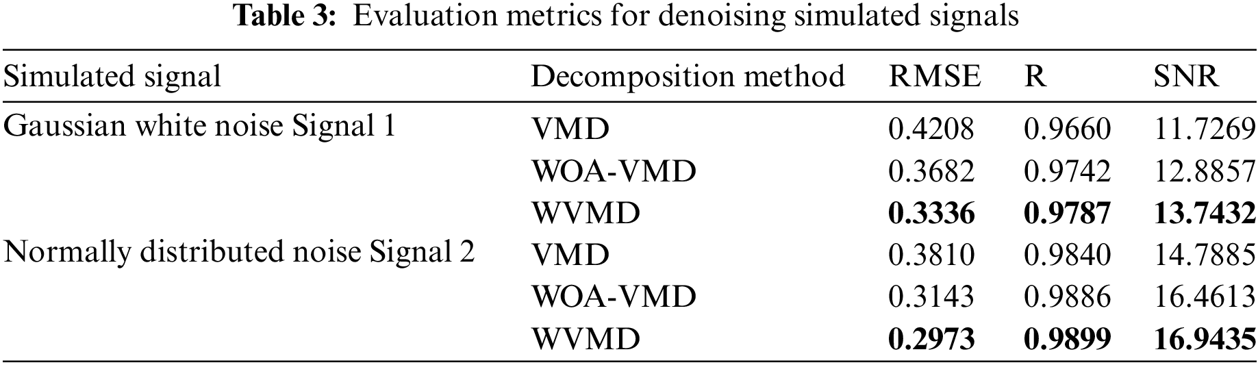
In this section, we compare the effectiveness of the WVMD technique with VMD and WOA-VMD. The comparison includes simulated signals with Gaussian white noise and signals with normally distributed noise. Simulated Signal 1 contains four distinct frequency components: a1, a2, a3, and a4, sampled at 500 Hz. The original signal is a superposition of a1, a2, a3, and a4. Signal 1 with noise includes Gaussian white noise with a signal-to-noise ratio of 10 dB, while Signal 2 with noise contains normally distributed noise with a signal-to-noise ratio of 15 dB. The Formula (15) as follows:

{ti=30π500⋅i, i∈[0, 499]a1=1.2cos⁡(0.1πti+π/4)a2=0.8sin⁡(0.3πti+π/6)a3=1.5cos⁡(0.5πti+π/3)a4=1.0sin⁡(0.7πti+π/2)s=a1+a2+a3+a4ξ=noise 1y=a1+a2+a3+a4+ξ{ti=30π500⋅i, i∈[0, 499]a1=1.5cos⁡(0.2πti+π/3)a2=1.0sin⁡(0.5πti+π/4)a3=2.0cos⁡(0.8πti+π/6)a4=1.2sin⁡(1.2πti+π/2)s=a1+a2+a3+a4ξ=noise 2y=a1+a2+a3+a4+ξ(15)

To verify the WVMD decomposition and denoising capabilities, we denoise the simulated signal by WVMD, WOA-VMD and VMD separately. The parameter combination [K, α] for VMD is [7, 500]. In Signal 1, the values of [K, α] for WOA-VMD are [3, 140], with a fitness value of 8.5471, and for WVMD are [10, 916], with a fitness value of 0.8965. In Signal 2, the values of [K, α] for WOA-VMD are [9, 532], with a fitness value of 8.6098, and for WVMD are [9, 334], with a fitness value of 1.1014. As shown in Table 3, the WVMD decomposition method outperforms WOA-VMD and VMD. Specifically, the WVMD-denoised signal has the highest SNR and R values and the lowest RMSE value. In both signals, compare the methods VMD and WOA-VMD, WVMD shows superior performance.

4.3.2 Decomposition Results Based on WVMD

To further improve the data quality and eliminate the effects of noise, WVMD is adopted to decompose the wind power dataset 1. The number of whales is set to 20, the maximum number of iterations is 40, the number of variables is 2, the penalty factor is [100, 2000], and the K value range is [2, 10] and includes only integers. From Fig. 4a, it can be seen that the whale algorithm is gradually stable after twelve iterations, and the optimal fitness function is 2.140759. The optimization curve of the penalty factor a is shown in Fig. 4c. After twelve iterations, the optimal penalty parameter is 619. From Fig. 4b, the optimal number for the IMF is 9. Fig. 5b shows the spectra of each IMF component. The time domain of modal components obtained by WVMD decomposition is presented in Fig. 5a.

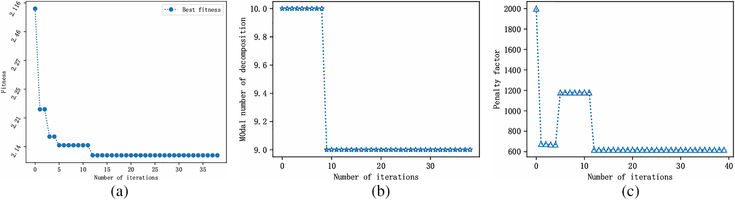
Figure 4: (a) Fitness curve of WVMD application in wind power; (b) Mode components K; (c) Penalty factor a

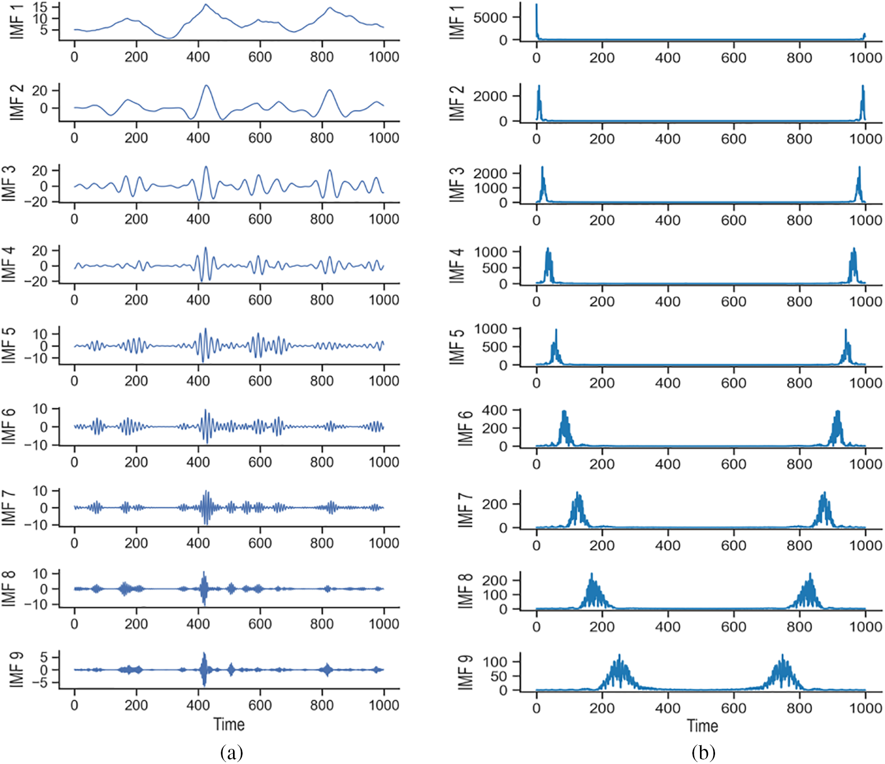
Figure 5: (a) WVMD decomposition of wind power; (b) Spectra of each IMF component

4.4 Comparison Analysis of WVMD_DSN

4.4.1 Ablation Study

In this section, using wind power generation datasets as an example, we validate the rationality of the WVMD_DSN model construction. As shown in Table 4, compared to the single models BiGRU and SENet, the hybrid model SENet-BiGRU shows an increase in RMSE and MAE by 11% and 11.5%, respectively. Similarly, compared to the hybrid model, the dual-stream model SENet-BiGRU exhibits an increase in RMSE and MAE by 4% and 8.3%, demonstrating the superior effectiveness of the DSN model over single and hybrid models. Incorporating WVMD as a preprocessing method before the DSN model notably enhances prediction accuracy, with RMSE, MAE, and NRMSE reaching as low as 1.1453, 0.8985, and 0.0056, respectively. Finally, the WVMD_DSN model, enhanced with attention mechanisms, achieves optimal performance with an RMSE of 1.0199 and an R2 value of 99.95%. The predictive performance of the WVMD_DSN method is illustrated in Fig. 6, showing that the predicted residuals consistently fluctuate around the zero scale line of the original wind power sequence.

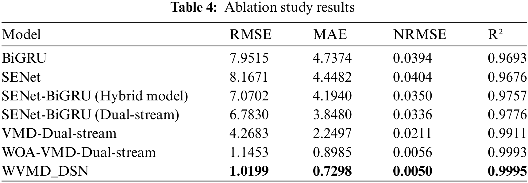
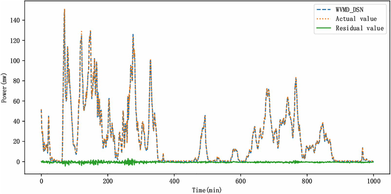
Figure 6: Prediction results and residual plot of WVMD_DSN

4.4.2 Comparison with Baseline Model

4.4.2.1 Comprehensive Analysis of the DSN Model

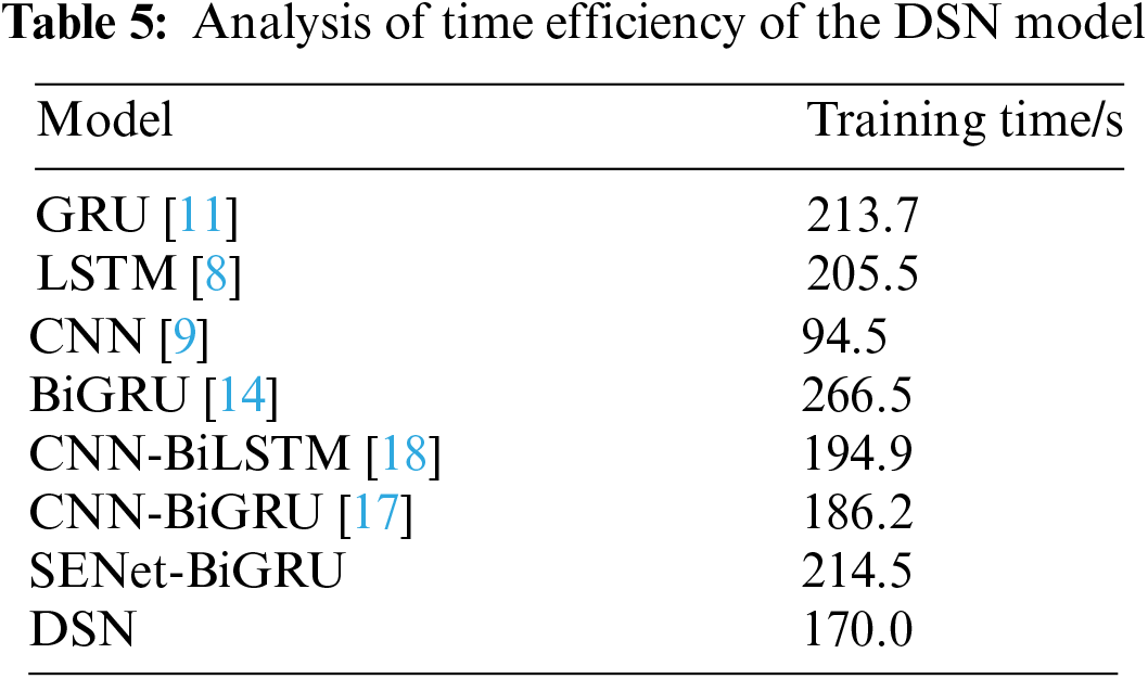
In this section, the proposed DSN model is analyzed in detail. According to Table 5, CNN has a training time of 94.5, making it the fastest among the models compared. CNN typically outperforms GRU and LSTM in processing sequence data because it uses parallel computing for feature mapping, rather than sequentially processing each element like recurrent neural networks. However, the RMSE and MAE of CNN alone are 9.2461 and 5.4185, respectively, indicating relatively poor prediction performance.

To address this, CNN is combined with BiGRU, CNN-BiLSTM, and other models. The CNN-BiGRU model has a shorter training period and higher prediction accuracy than BiGRU. This improvement is due to CNN’s ability to effectively extract features from input data, especially when dealing with spatially structured data. By incorporating CNN, the output feature maps become more concise and representative, which reduces the data and complexity that BiGRU needs to handle. Although combining CNN with SENet and BiGRU improves prediction performance, it also increases time complexity. This is mainly because SENet includes an attention mechanism, which adds more parameters and complexity to the model.

Compared to GRU, BiGRU, and CNN-BiGRU, the DSN model shows improved prediction accuracy. However, its training cycle increases by 20.4%, 36.1%, and 8.6%, respectively. RMSE rises by 21.1%, 14.6%, and 8.3%, while MAE increases by 31.6%, 18.7%, and 16.6%. Overall, DSN offers advantages in terms of prediction accuracy despite a longer training time.

Compare the Proposed WVMD_DSN Model

We compare the proposed WVMD_DSN model with other commonly used similar algorithms. The specific results are detailed in Table 6. The WVMD_DSN method shows improvements compared to single models GRU, CNN, and LSTM, with R2 increasing by 3.7%, 4.2%, and 3.5%, respectively, and RMSE increasing by 7, 8, and 8 percentage points. MAE also increases by 5, 4.9, and 4.8 percentage points. Compared to the hybrid model CNN-BiLSTM, WVMD_DSN increases RMSE by around 6 percentage points, improves R2 by 2.6%, and increases MAE by 3.7 percentage points. Similarly, compared to other hybrid models, WVMD_DSN shows corresponding improvements in RMSE, MAE, NRMSE, and R2. This validates that WVMD_DSN performs better than single models and hybrid models for wind power prediction. Compared to the original DSN, WVMD_DSN increases RMSE by approximately 5 percentage points, improves R2 by 2.3%, and increases MAE by 2.9 percentage points. Therefore, the proposed WVMD_DSN model demonstrates superior predictive accuracy. The two streams of DSN proposed in this paper consist of SENet and BiGRU. The Table 6 shows that BiGRU has an RMSE 7.5% and 12.9% higher than GRU and LSTM, respectively. Thus, BiGRU is preferred for the second stream to handle wind power time series data. SENet, which is an improvement over CNN, has an RMSE 11.6% higher than CNN. Therefore, SENet is better for the first stream to capture spatial characteristics of wind power. An attention mechanism is then used to remove redundant data from both streams. Finally, combined with WVMD preprocessing technology, this approach shows a greater improvement compared to DSN alone. The prediction results are depicted in Fig. 7, showing substantial overlap between the WVMD_DSN approach and the original sequences, indicating its superior predictive performance.

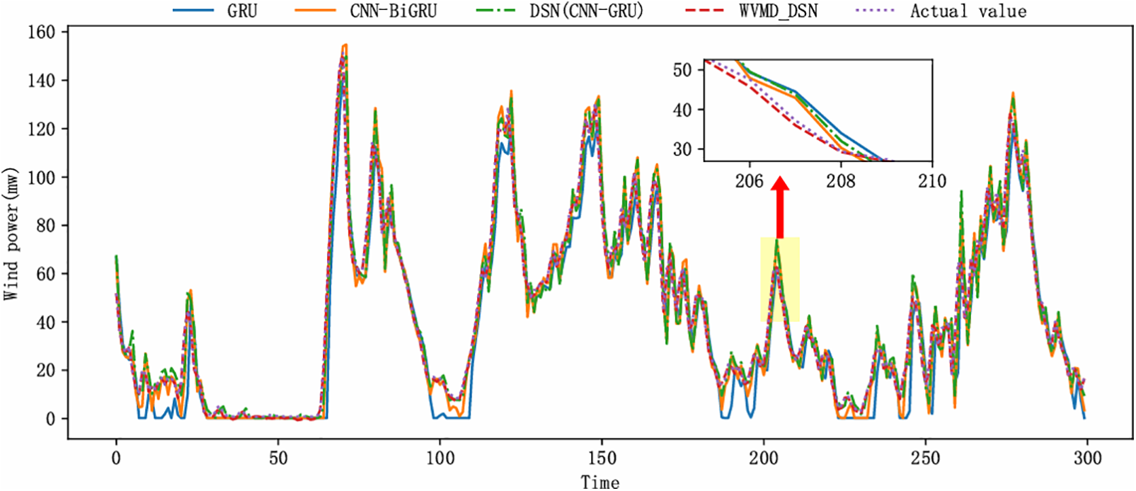
Figure 7: Prediction results and residual plot of WVMD_DSN

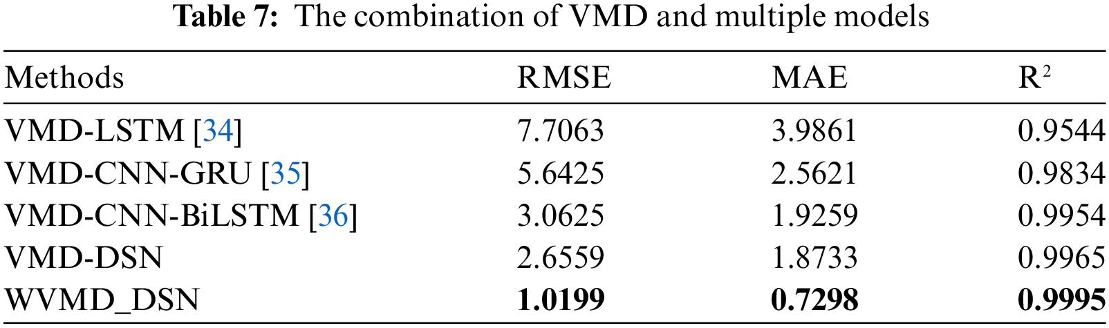
Compare the Combination of VMD with Multiple Models

The parameter settings for VMD and model parameters remain consistent with those previously described. VMD is combined with LSTM, CNN-LSTM, CNN-GRU, CNN-BiLSTM, and DSN, as shown in Table 7. These combinations significantly enhance prediction accuracy, with the DSN model demonstrating superior performance. Compared to LSTM, CNN-LSTM, CNN-GRU, and CNN-BiLSTM, integrating VMD with DSN results in RMSE increases of 65.5%, 26.9%, and 13.3%, respectively, MAE increases of 53%, 26.9%, and 2.7%, respectively, and R2 increases of 4.4%, 1.3%, and 0.11%, respectively. This further confirms the DSN model’s superiority in wind power prediction. Additionally, using WOA optimization further enhances prediction accuracy when combining VMD with DSN.

4.4.3 Generalization Analysis

In this section, the generalization ability of the WVMD_DSN model is primarily examined by using a wind power dataset 2. The optimized parameters (K, a) obtained from WVMD are (8, 100). Comparative evaluation metrics performance of WVMD_DSN and baseline models are shown in Table 8. It can be observed that WVMD_DSN achieves an RMSE of 0.3704 and MAE of 0.2593. Compared to the single GRU model, these represent improvements of 89.6% and 88.9%, respectively. Compared to the hybrid CNN-BiGRU model, WVMD_DSN improves by 84.9% and 70.5%, and compared to the DSN model, improvements are 83.2% and 66.8%, respectively. The WVMD_DSN model continues to demonstrate superior performance on wind power dataset 2, highlighting its strong generalization capability.

5  Conclusion and Future Work

The paper proposes a short-term wind power prediction method that integrates WVMD with a novel DSN model. The main conclusions are as follows:

(1)   Through experiments on actual wind power data, it is shown that WVMD can address the adaptiveness in selecting the mode number K and penalty factor a more effectively.

(2)   The paper proposes a novel DSN model, which combines AM and SENet-BiGRU, demonstrating a significant improvement in the accuracy of wind power prediction. When combined with the WVMD preprocessing method, the effectiveness of wind power forecasting is further enhanced. Moreover, to verify the generalization capability of the WVMD_DSN method, experiments were conducted using real wind power dataset 2, which also exhibit volatility and instability, fully proving that WVMD_DSN has excellent generalization ability.

(3)   After a comprehensive analysis, the improved DSN model outperforms GRU, BiGRU, and CNN-BiGRU in both training time and prediction accuracy. While DSN shows better prediction accuracy, its training times increase by 20.4%, 36.1%, and 8.6% compared to GRU, BiGRU, and CNN-BiGRU, respectively. RMSE and MAE also increase by 21.1%, 14.6%, and 8.3% and 31.6%, 18.7%, and 16.6%, respectively. This model effectively enhances grid reliability and security and reduces scheduling time for integrating renewable energy into the power grid.

In the future, we will utilize some adaptive optimization algorithms to consider the learning rate and batch size parameters of the DSN network model. Additionally, we will use various data sources to improve the wind power generation forecasting model, including meteorological data, GIS data, wind farm layout data, and real-time monitoring data.

Acknowledgement: I am especially grateful to my teacher for her guidance and support in my research work. I also want to thank my laboratory colleagues for their help and suggestions throughout the research process.

Funding Statement: This work was supported in part by the Science and Technology Project of State Grid Corporation of China under Grant 5400-202117142A-0-0-00, the National Natural Science Foundation of China under Grant 62372242.

Author Contributions: The authors confirm contribution to the paper as follows: study conception and design: Yingnan Zhao, Yuyuan Ruan; data collection: Zhen Peng; analysis and interpretation of results: Yuyuan Ruan; draft manuscript preparation: Yuyuan Ruan, Yingnan Zhao. All authors reviewed the results and approved the final version of the manuscript.

Availability of Data and Materials: The data that support the findings of this study are openly available in Wind-power-forecast at https://github.com/ruanyuyuan/Wind-power-forecast.git (accessed on 20 August 2024).

Ethics Approval: Not applicable.

Conflicts of Interest: The authors declare that they have no conflicts of interest to report regarding the present study.

References

1. M. S. Ko, K. Lee, J. K. Kim, C. W. Hong, Z. Y. Dong and K. Hur, “Deep concatenated residual network with bidirectional LSTM for one-hour-ahead wind power forecasting,” IEEE Trans. Sustain. Energy, vol. 12, no. 2, pp. 1321–1335, 2021. doi: 10.1109/TSTE.2020.3043884. [Google Scholar] [CrossRef]

2. J. Yan, H. Zhang, Y. Liu, S. Han, L. Li and Z. Lu, “Forecasting the high penetration of wind power on multiple scales using multi-to-multi mapping,” IEEE Trans. Power Syst., vol. 33, no. 3, pp. 3276–3284, 2017. doi: 10.1109/TPWRS.2017.2787667. [Google Scholar] [CrossRef]

3. Z. Li et al., “A spatiotemporal directed graph convolution network for ultra-short-term wind power prediction,” IEEE Trans. Sustain. Energy, vol. 14, no. 1, pp. 39–54, 2023. doi: 10.1109/TSTE.2022.3198816. [Google Scholar] [CrossRef]

4. P. Guo, Y. Gan, and D. Infield, “Wind turbine performance degradation monitoring using DPGMM and Mahalanobis distance,” Renew. Energy, vol. 200, pp. 1–9, 2022. doi: 10.1016/j.renene.2022.09.115. [Google Scholar] [CrossRef]

5. G. M. Shafiullah, M. T. Amanullah, A. B. Shawkat, P. Wolfs, and M. T. Arif, “Renewable energy integration: Opportunities and challenges,” in Ali. Smart Grids. Green Energy and Technology. London: Springer, pp. 45–76, 2013. [Google Scholar]

6. J. Heinermann and O. Kramer, “Machine learning ensembles for wind power prediction,” Renew. Energy, vol. 89, pp. 671–679, 2016. doi: 10.1016/j.renene.2015.11.073. [Google Scholar] [CrossRef]

7. I. Khabbouchi, I. B. Salem, M. S. Guellouz, and U. Ritschel, “Machine learning and deep learning for wind power forecasting,” in 2023 IEEE Int. Conf. Artif. Intell. Green Energy (ICAIGE), Sousse, Tunisia, 2023, pp. 1–6. [Google Scholar]

8. T. Ahmad and D. D. Zhang, “A data-driven deep sequence-to-sequence long-short memory method along with a gated recurrent neural network for wind power forecasting,” Energy, vol. 239, 2022, Art. no. 122109. doi: 10.1016/j.energy.2021.122109. [Google Scholar] [CrossRef]

9. M. A. Hossain, R. K. Chakrabortty, S. Elsawah, and M. J. Ryan, “Very short-term forecasting of wind power generation using hybrid deep learning model,” J. Clean. Prod., vol. 296, 2021, Art. no. 126564. doi: 10.1016/j.jclepro.2021.126564. [Google Scholar] [CrossRef]

10. Y. Y. Hong and C. Rioflorido, “A hybrid deep learning-based neural network for 24-h ahead wind power forecasting,” Appl. Energy, vol. 250, pp. 530–539, 2019. doi: 10.1016/j.apenergy.2019.05.044. [Google Scholar] [CrossRef]

11. P. Lu, L. Ye, Y. Zhao, B. Dai, M. Pei and Y. Tang, “Review of meta-heuristic algorithms for wind power prediction: Methodologies, applications and challenges,” Appl. Energy, vol. 301, 2021, Art. no. 117446. doi: 10.1016/j.apenergy.2021.117446. [Google Scholar] [CrossRef]

12. A. Meng et al., “A novel few-shot learning approach for wind power prediction applying secondary evolutionary generative adversarial network,” Energy, vol. 261, 2022, Art. no. 125276. doi: 10.1016/j.energy.2022.125276. [Google Scholar] [CrossRef]

13. A. A. Ezzat, M. Jun, and Y. Ding, “Spatio-temporal short-term wind forecast: A calibrated regime-switching method,” Ann. Appl. Stat., vol. 13, no. 3, pp. 1484–1510, 2019. doi: 10.1214/19-AOAS1243. [Google Scholar] [PubMed] [CrossRef]

14. A. A. Ezzat, M. Jun, and Y. Ding, “Spatio-temporal asymmetry of local wind fields and its impact on short-term wind forecasting,” IEEE Trans. Sustain. Energy, vol. 9, no. 3, pp. 1437–1447, 2018. doi: 10.1109/TSTE.2018.2789685. [Google Scholar] [PubMed] [CrossRef]

15. S. Hu et al., “Hybrid forecasting method for wind power integrating spatial correlation and corrected numerical weather prediction,” Appl. Energy, vol. 293, 2021, Art. no. 116951. doi: 10.1016/j.apenergy.2021.116951. [Google Scholar] [CrossRef]

16. J. Zhang et al., “Power prediction of a wind farm cluster based on spatiotemporal correlations,” Appl. Energy, vol. 302, 2021, Art. no. 117568. doi: 10.1016/j.apenergy.2021.117568. [Google Scholar] [CrossRef]

17. Y. Chen et al., “CNN-BiLSTM short-term wind power forecasting method based on feature selection,” IEEE J. Radio Freq. Identif., vol. 6, pp. 922–927, 2022. doi: 10.1109/JRFID.2022.3213753. [Google Scholar] [CrossRef]

18. Z. Ma and G. Mei, “A hybrid attention-based deep learning approach for wind power prediction,” Appl. Energy, vol. 323, 2023, Art. no. 119608. doi: 10.1016/j.apenergy.2022.119608. [Google Scholar] [CrossRef]

19. K. Simonyan and A. Zisserman, “Two-stream convolutional networks for action recognition in videos,” In: Advances in Neural Information Processing Systems 27 (NIPS 2014), Curran Associates, Inc., 2014, vol. 27, pp. 568–576. [Google Scholar]

20. B. Su, P. Zhang, M. Sun, and M. Sheng, “Direction-guided two-stream convolutional neural networks for skeleton-based action recognition,” Soft Comput., vol. 27, pp. 11833–11842, 2023. doi: 10.1007/s00500-023-07862-1. [Google Scholar] [CrossRef]

21. Z. A. Khan, T. Hussain, and S. W. Baik, “Dual stream network with attention mechanism for photovoltaic power forecasting,” Appl. Energy, vol. 338, 2023, Art. no. 120916. doi: 10.1016/j.apenergy.2023.120916. [Google Scholar] [CrossRef]

22. W. Zhang, F. Liu, X. Zheng, and Y. Li, “A hybrid EMD-SVM based short-term wind power forecasting model,” in 2015 IEEE PES Asia-Pacific Power Energy Eng. Conf. (APPEEC), Brisbane, QLD, Australia, 2015, pp. 1–5. [Google Scholar]

23. S. Wang, N. Zhang, L. Wu, and Y. Wang, “Wind speed forecasting based on the hybrid ensemble empirical mode decomposition and GA-BP neural network method,” Renew. Energy, vol. 94, pp. 629–636, 2016. doi: 10.1016/j.renene.2016.03.103. [Google Scholar] [CrossRef]

24. I. Daubechies, “The wavelet transform time-frequency localization and signal analysis,” IEEE Trans. Inf. Theory, vol. 36, no. 5, pp. 961–1005, 1990. doi: 10.1109/18.57199. [Google Scholar] [CrossRef]

25. K. Dragomiretskiy and D. Zosso, “Variational mode decomposition,” IEEE Trans. Signal Process., vol. 62, no. 3, pp. 531–544, Feb. 1, 2014. doi: 10.1109/TSP.2013.2288675. [Google Scholar] [CrossRef]

26. N. Rehman and D. P. Mandic, “Empirical mode decomposition for trivariate signals,” IEEE Trans. Signal Process., vol. 58, no. 3, pp. 1059–1068, 2010. doi: 10.1109/TSP.2009.2033730. [Google Scholar] [CrossRef]

27. X. Gao, W. Guo, C. Mei, J. Sha, Y. Guo and H. Sun, “Short-term wind power forecasting based on SSA-VMD-LSTM,” Energy Rep., vol. 9, pp. 335–344, 2023. doi: 10.1016/j.egyr.2023.05.181. [Google Scholar] [CrossRef]

28. S. Mirjalili and A. Lewis, “The whale optimization algorithm,” Adv. Eng. Softw., vol. 95, pp. 51–67, 2016. doi: 10.1016/j.advengsoft.2016.01.008. [Google Scholar] [CrossRef]

29. D. Wang, D. Tang, and L. Liu, “Particle swarm optimization algorithm,” Soft Comput., vol. 22, pp. 387–408, 2018. doi: 10.1007/s00500-016-2474-6. [Google Scholar] [CrossRef]

30. S. Mirjalili, S. M. Mirjalili, and A. Lewis, “Grey wolf optimizer,” Adv. Eng. Softw., vol. 69, pp. 46–61, 2014. doi: 10.1016/j.advengsoft.2013.12.007. [Google Scholar] [CrossRef]

31. N. Kwak and C. H. Choi, “Input feature selection for classification problems,” IEEE Trans. Neural Netw., vol. 13, pp. 143–159, 2002. [Google Scholar] [PubMed]

32. J. Hu, L. Shen, and G. Sun, “Squeeze-and-excitation networks,” in 2018 IEEE/CVF Conf. Comput. Vis. Pattern Recognit., Salt Lake City, UT, USA, 2018, pp. 7132–7141. [Google Scholar]

33. K. Cho, B. Merriënboer, D. Bahdanau, and Y. Bengio, “On the properties of neural machine translation: Encoder-decoder approaches,” in 8th Workshop Syntax, Semant. Struct. Stat. Transl., SSST 2014, Doha, Qatar, 2014, pp. 103–111. doi: 10.3115/v1/W14-40. [Google Scholar] [CrossRef]

34. L. Han, R. Zhang, X. Wang, A. Bao, and H. Jing, “Multi-step wind power forecast based on VMD-LSTM,” IET Renew. Power Gener., vol. 13, pp. 1609–1700, 2019. doi: 10.1049/iet-rpg.2018.5781. [Google Scholar] [CrossRef]

35. Z. Zhao et al., “Hybrid VMD-CNN-GRU-based model for short-term forecasting of wind power considering spatio-temporal features,” Eng. Appl. Artif. Intell., vol. 121, 2023, Art. no. 105982. doi: 10.1016/j.engappai.2023.105982. [Google Scholar] [CrossRef]

36. Y. Dai, R. Wang, Y. Ma, T. Wan, and Z. Huang, “Research on CNN-BiLSTM power load forecasting based on VMD algorithm,” in 2023 IEEE 5th Int. Conf. Civil Aviation Saf. Inform. Technol. (ICCASIT), Dali, China, 2023, pp. 1098–1102. [Google Scholar]