An Efficient Long Short-Term Memory and Gated Recurrent Unit Based Smart Vessel Trajectory Prediction Using Automatic Identification System Data

1  Introduction

Ship navigation presents unique challenges compared to vehicular transport. The absence of predefined paths for ships makes trajectory prediction a complex task [1]. Traditional methods relying on dynamic equation construction for predicting ship paths were limited by their dependence on extensive expert knowledge and lack of adaptability to diverse scenarios.

In recent years, machine learning has emerged as a preferred approach for ship trajectory prediction. This shift is attributed to machine learning’s superior adaptability, achieved through its capacity to learn from both historical and real-time driving trajectories [2].

Automatic Identification System (AIS) data plays a crucial role in modern maritime navigation, providing essential real-time trajectory information. This data is instrumental in monitoring ship movements, triggering collision avoidance alerts, ensuring maritime safety, and facilitating accident investigations. Typically comprising time and location information, AIS data is visualized on electronic charts, enabling effective tracking of ship trajectories [3,4].

The AIS technology serves as one of the most important pillars in navigation systems, offering abundant near-real-time maritime positioning data [5]. It integrates the Maritime Mobile Service Identity (MMSI) with crucial navigational parameters including longitude, latitude, speed, course, and additional contextual information [6]. This comprehensive AIS dataset enables the tracking of a vast majority of vessels and facilitates the extraction of ship navigation patterns. Moreover, time series analysis can be employed to compare the emerging patterns among various maritime trajectories [7].

In regions with high maritime traffic and challenging conditions, enhancing ship safety is paramount. Vessel Traffic Service (VTS) plays a crucial role by accurately monitoring and predicting ship trajectories in real time, aiding in the early detection of potential marine accidents. Improving ship safety in dynamic and complex sea environments [8] requires integrating trajectory prediction and hazard warning capabilities into ships’ intelligent navigation systems. However, maritime navigation is inherently unpredictable, particularly in congested port waters, making it challenging to anticipate the movements of vessels. Predicting trajectories accurately and efficiently in real-time is a significant challenge. This task spans various domains, including flight, human, and vehicle trajectory prediction [3,9–11]. Trajectory data combine spatial and temporal dimensions, making them unique time series datasets. Traditionally, Kalman filters have been used to forecast ship trajectories based on waypoints.

Two methods are used in the literature for vessel trajectory prediction: Physical models and Learning models. Initial techniques rely on physical models of vessel motion, primarily employing ship models [12,13] and lateral models [5,14]. These approaches represent the physical movement of ships using a combination of mathematical equations and principles that consider factors such as mass, size, inertia, and center of mass. However, the accuracy of these methods is contingent upon precise representations of environmental conditions and assumptions about the vessel’s state, which are often difficult to achieve in practical vessel trajectory prediction scenarios.

In contrast to physical model-based approaches [15,16], learning model-based methods for vessel trajectory prediction rely on machine learning techniques. These methods utilize data-driven models, such as neural networks, to learn patterns and relationships from historical trajectory data. By leveraging large datasets, learning model-based methods aim to capture complex interactions and dynamics inherent in vessel movements. This approach offers the potential for improved accuracy and adaptability in predicting vessel trajectories, particularly in scenarios where precise physical modeling is challenging.

One prominent technique within this paradigm is the Kalman Filter. For instance, Kalman Filter techniques utilize dynamic data from vessel targets, eliminating noise to predict the subsequent locations of vessels [17]. Siegert et al. [18] employed an Extended Kalman Filter (EKF) to monitor vessel trajectories, enabling failure detection through residual monitoring. Additionally, in another study, an Extended Kalman Filter was proposed as an adaptive algorithm to estimate position, velocity, and acceleration for predicting maneuvers in ocean vessel trajectories [3].

The Extended Kalman Filter has been extensively studied and successfully applied in various contexts, providing a wealth of resources for exploitation. However, it’s worth noting that while powerful, the Extended Kalman Filter may not always yield globally optimal results, highlighting the ongoing need for research in this area.

The emergence of deep learning techniques, including convolutional neural networks [19], recurrent neural networks (RNNs) [20] and variational autoencoders [21–23] has led to significant advancements in generalization performance for trajectory prediction tasks. Several machine learning-based methods [24–26] have emerged, such as the backpropagation (BP) neural network, Long Short-Term Memory (LSTM) model [4],and the Attention-LSTM ship trajectory prediction model. Kaiser et al. [27] utilized Automatic Identification System (AIS) data to enhance port traffic management, while Ahmed et al. [28] employed artificial neural networks for automated ship berthing, using two distinct feedforward networks to control rudder angle and propeller rotation. Zissis et al. [29] combined Artificial Neural Networks (ANNs) with cloud computing for real-time ship behavior prediction.

A significant advancement in the field is the fusion of Automatic Identification System (AIS) data with backpropagation neural networks to enhance ship navigation behavior prediction. Concurrently, the LSTM model, a variant of recurrent neural networks, has demonstrated remarkable efficacy in discerning ship motion patterns for trajectory forecasting. Moreover, the traditional Encoder-Decoder framework for trajectory prediction has undergone substantial refinement through the integration of longitudinal attention mechanisms and the incorporation of historical positional data, thereby augmenting its predictive capabilities.

In this paper, an advanced trajectory prediction system leveraging LSTM and GRU models for smart vessel navigation is proposed. The system utilizes Automatic Identification System (AIS) data, incorporating latitude, longitude, speed, and heading information as inputs for LSTM and GRU models to forecast vessel trajectories. The validation process, conducted over a three-month AIS dataset, demonstrates notable performance improvements.

Specifically, for GRU, the training loss is reduced by 0.0334 (Mean Squared Error, MSE) and 0.1361 (Mean Absolute Error, MAE), with validation loss reaching 0.0708 (MSE) and 0.1720 (MAE). Similarly, LSTM exhibits reduced training loss of 0.0632 (MSE) and 0.1702 (MAE), along with validation loss decreasing to 0.2290 (MSE) and 0.2652 (MAE). The main objectives of the paper are as follows:

•   Develop an advanced trajectory prediction system for smart vessel navigation.

•   Utilize LSTM, GRU, DBLSTM, and Simple RNN models for trajectory forecasting.

•   Incorporate Automatic Identification System (AIS) data, including latitude, longitude, speed, and heading information, as inputs.

•   Conduct validation using a three-month AIS dataset to assess performance improvements.

•   Compare the performance of LSTM, GRU, DBLSTM, and SimpleRNN models based on MSE, MAE, ADE, and FDE metrics.

The rest of the paper is structured as follows: Section 2 defines the proposed methodology with subsection of LSTM and GRU. Sections 3 and 4 describe the complete implementation and results with brief discussion, and finally, the paper is concluded in Section 5.

2  Methodology

The proposed framework is designed with precision to sequentially process raw Automatic Identification System (AIS) data, focusing on the extraction, preprocessing, and predictive analysis of vessel trajectories. Initially, the framework employs a complex extraction algorithm as illustrated in Fig. 1 to filter through the extensive AIS-dataset and extracts the data through two distinct approaches.

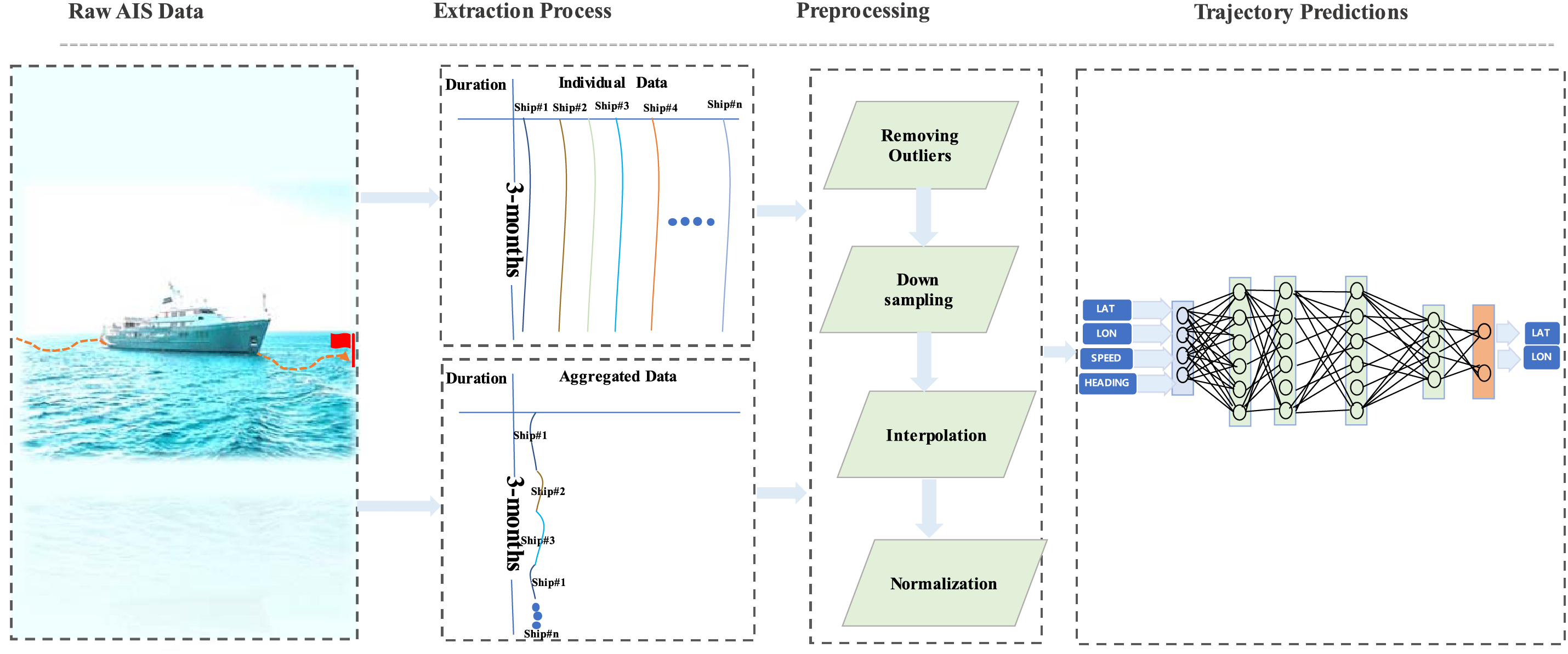
Figure 1: Abstract trajectory prediction model with data preprocessing steps

The first approach involves extracting individual ship data over a three-month period. This method ensures that the privacy of each ship is maintained, as the data remains isolated and more concise. Due to the smaller dataset size, simpler models that require less data can be effectively utilized, providing precise and efficient analysis for each ship.

The second approach aggregates data from all ships into a single, comprehensive dataset, resulting in a significantly larger data volume. This aggregated dataset facilitates a more holistic analysis of ship trajectories but necessitates the use of more complex models that can handle large-scale data to derive meaningful insights.

This dual extraction method is crucial for accurately isolating trajectories associated with each ship, thereby ensuring the precision of the data used in subsequent analyses. Following extraction, each trajectory undergoes a rigorous preprocessing sequence aimed at eliminating anomalies and outliers, thereby preserving the integrity and reliability of the data. This thorough preprocessing is essential for maintaining the quality and accuracy of the predictive analyses that follow.

The framework utilizes raw Automatic Identification System (AIS) data for preprocessing and subsequent vessel trajectory prediction. Two deep learning models, Gated Recurrent Unit (GRU) and Long Short-Term Memory (LSTM) networks, are employed for the prediction process. The raw AIS data is first preprocessed to obtain clean data, which is then used as input for trajectory prediction.

GRU and LSTM models are applied for predicting vessel trajectories, chosen for their renowned efficiency in processing and predicting sequential data patterns compared to other deep learning models. This approach underscores the framework’s focus on improving the accuracy and reliability of trajectory predictions in maritime navigation. Finally, the model performance is evaluated using Root Mean Square Error (RMSE) and Mean Absolute Error (MAE) metrics for vessel trajectory prediction.

The framework is constructed on the foundation of raw AIS data, which undergoes preprocessing before being utilized for vessel trajectory prediction. The prediction methodology incorporates multiple deep learning techniques, including GRU, LSTM networks, BDLSTM, and Simple RNN, all renowned for their proficiency in processing and predicting sequential data patterns. For comparative analysis, traditional methods such as the Kalman Filter were also implemented. The preprocessed AIS data serves as input for all trajectory prediction models. The vessel trajectory prediction is executed through the application of these advanced neural network models, emphasizing the framework’s focus on enhancing the accuracy and reliability of trajectory predictions in maritime navigation.

The model’s performance is assessed using a diverse set of evaluation metrics: Root Mean Square Error (RMSE), Mean Absolute Error (MAE), Average Displacement Error (ADE), and Final Displacement Error (FDE) for vessel trajectory prediction. The incorporation of ADE and FDE metrics offers a more comprehensive evaluation framework for the prediction models by quantifying both the average trajectory accuracy and the terminal position accuracy, respectively. This multifaceted approach to performance assessment is particularly relevant in maritime navigation contexts, where both continuous path accuracy and final destination precision are crucial.

Section 4.2 presents a comparative analysis that demonstrates the superior performance of the Gated Recurrent Unit (GRU) model across the majority of datasets. The GRU produces lower values for Test Loss, Mean Squared Error (MSE), Mean Absolute Error (MAE), Average Displacement Error (ADE), and Final Displacement Error (FDE) relative to other models, including Long Short-Term Memory (LSTM), Bidirectional LSTM (BDLSTM), Simple Recurrent Neural Network (SimpleRNN), and the Kalman Filter. These results demonstrate the GRU’s effectiveness in capturing temporal dependencies and generating accurate predictions. Furthermore, this comparison emphasizes the critical importance of selecting appropriate models based on the specific characteristics of the dataset and the unique requirements of the application domain.

2.1 GRU Model for Trajectory Prediction

Recurrent Neural Networks (RNNs) are a specialized class of neural networks designed for processing sequential data, characterized by their cyclically connected units [30]. While RNNs are frequently employed for short-term prediction tasks, they are prone to the gradient vanishing problem during training. To mitigate this limitation, Chung et al. [31] introduced the Gated Recurrent Unit (GRU) model as an enhancement to conventional RNNs. GRU incorporates the hidden layer state concept from RNNs and shares architectural similarities with Long Short-Term Memory (LSTM) models. However, GRU offers improved computational efficiency compared to LSTM by combining the forget and input gates into a unified update gate. This design enables GRU to effectively retain historical time-series information. Through its gating mechanism, GRU can preserve past trajectory information while reducing computational complexity. In contrast to LSTM, GRU features a more streamlined hierarchical structure and fewer parameters, yet it can achieve comparable performance. Fig. 2 illustrates the fundamental principles underlying the GRU structure.

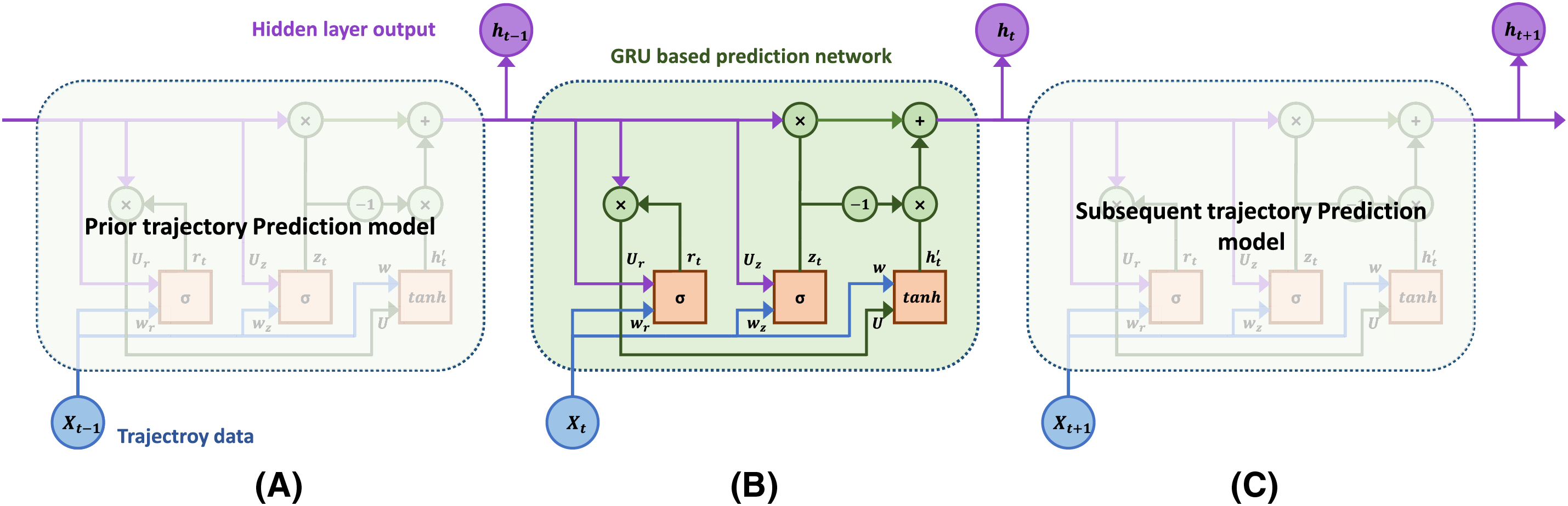
Figure 2: Schematic representation of an abstract trajectory prediction model based on the Gated Recurrent Unit (GRU) neural network architecture: (a) The GRU unit at time step t − 1; (b) Detailed internal structure of the GRU unit at the current time step t, illustrating the complex transition mechanisms; and (c) The GRU unit at the subsequent time step t + 1

To comprehensively analyze the mechanics of the Gated Recurrent Unit (GRU) neural network architecture, it is essential to examine the dynamics of its hidden layer. When processing an input sequence denoted xi (for i=1, 2,…,n), the hidden layer’s state at any given time step i can be characterized by the following formulation:

ui=σ(Vu⋅[gi−1, xi])(1)

yi=σ(Vy⋅[gi−1, xi])(2)

g^i=tanh⁡(V⋅[ui⊙gi−1, xi])(3)

gi=(1−yi)⊙gi−1+yi⊙g^i(4)

Here, σ represents the sigmoid function (σ(x)=11+e−x), and tanh⁡(x)=e2x−1e2x+1. The notation [] signifies the concatenation of two vectors, ⊙ denotes element-wise multiplication, and ⋅ symbolizes matrix multiplication, expressed as:

a⊙b=[a1a2a3⋮an]⊙[b1b2b3⋮bn]=[a1b1a2b2a3b3⋮anbn]

The training of the GRU network at time i involves optimizing the weight matrices Vu, Vy, and V, which are each a sum of two distinct weight matrices as follows:

Vu=Vux+Vug(5)

Vy=Vyx+Vyg(6)

V=Vx+Vg(7)

The weight matrices Vux, Vyx, and Vx establish the connections between the input and the update gate, reset gate, and candidate state, respectively. Concurrently, the matrices Vug, Vyg, and Vg facilitate the connections from the previous hidden state to the update gate y, the reset gate u, and the candidate state g^, in that order.

A higher value of yi at any time i means the state gi−1 from the previous timestep influences the current state gi less, and the candidate state g^i has more impact. Conversely, a value of yi close to 1 indicates that the previous state gi−1 has a significant contribution to the current state gi. This mechanism allows the GRU to capture dependencies over longer sequences effectively. Similarly, a higher value of ui enhances the influence of the candidate state g^i on the update process, enabling the model to incorporate information from further back in the sequence. If ui is near zero, it suggests that the past state gi−1 has little to no effect on the candidate state g^i, emphasizing the model’s capacity to prioritize recent information over older data in the sequence analysis.

The Gated Recurrent Unit (GRU) architecture represents an evolution of the Long Short-Term Memory (LSTM) model. It merges the LSTM’s forget gate f and input gates i into a single update gate zi. Additionally, it combines the hidden and cell states of the LSTM, introducing a reset gate ri. The role of the reset gate ri is crucial as it regulates how much information from previous time steps is permitted to contribute to the current hidden state, particularly concerning the navigation path of a vessel. The update gate zi plays a key role in incorporating past state information into the current state. It manages how new trajectory data and past memories are combined to determine the pertinent information for the current state, which is then used to compute the state information for the ensuing time step. By carefully applying the GRU’s gating mechanisms, essential data is preserved, thus preventing information decay over long data propagation intervals. The GRU’s inherently efficient design requires fewer parameters to be learned, which translates to a faster training process for the model.

2.2 LSTM Model for Trajectory Prediction

The neural network (NN) proposed integrates a LSTM component with a single-hidden layer Multilayer Perceptron (MLP). The LSTM is adept at leveraging historical data insights. The MLP, despite its limitations in dynamic environments, offers a streamlined architecture ideal for capturing localized features. Despite the MLP’s known limitations in dynamic environments, its simplicity and effectiveness have led to pervasive utilization across various domains. The NN model in question consists of an input layer, which introduces features as defined by Eq. (11), an LSTM layer for temporal processing, a fully-connected layer for feature integration, and an output layer that generates two features as specified in Eq. (24).

This architecture employs a conventional LSTM configuration, incorporating three gates as detailed in [32]. The model is specifically designed to address the challenges inherent in processing asynchronous, time-sampled spatiotemporal data, aligning with the proposed spatiotemporal-aware methodology outlined in Eqs. (8)–(10). Fig. 3 presents a comprehensive depiction of the architecture, illustrating the LSTM model’s four input data streams and its ultimate output in the form of latitude and longitude coordinates. This structure enables the network to effectively capture and process complex spatiotemporal relationships within the input data, facilitating accurate predictions in a geographic context.

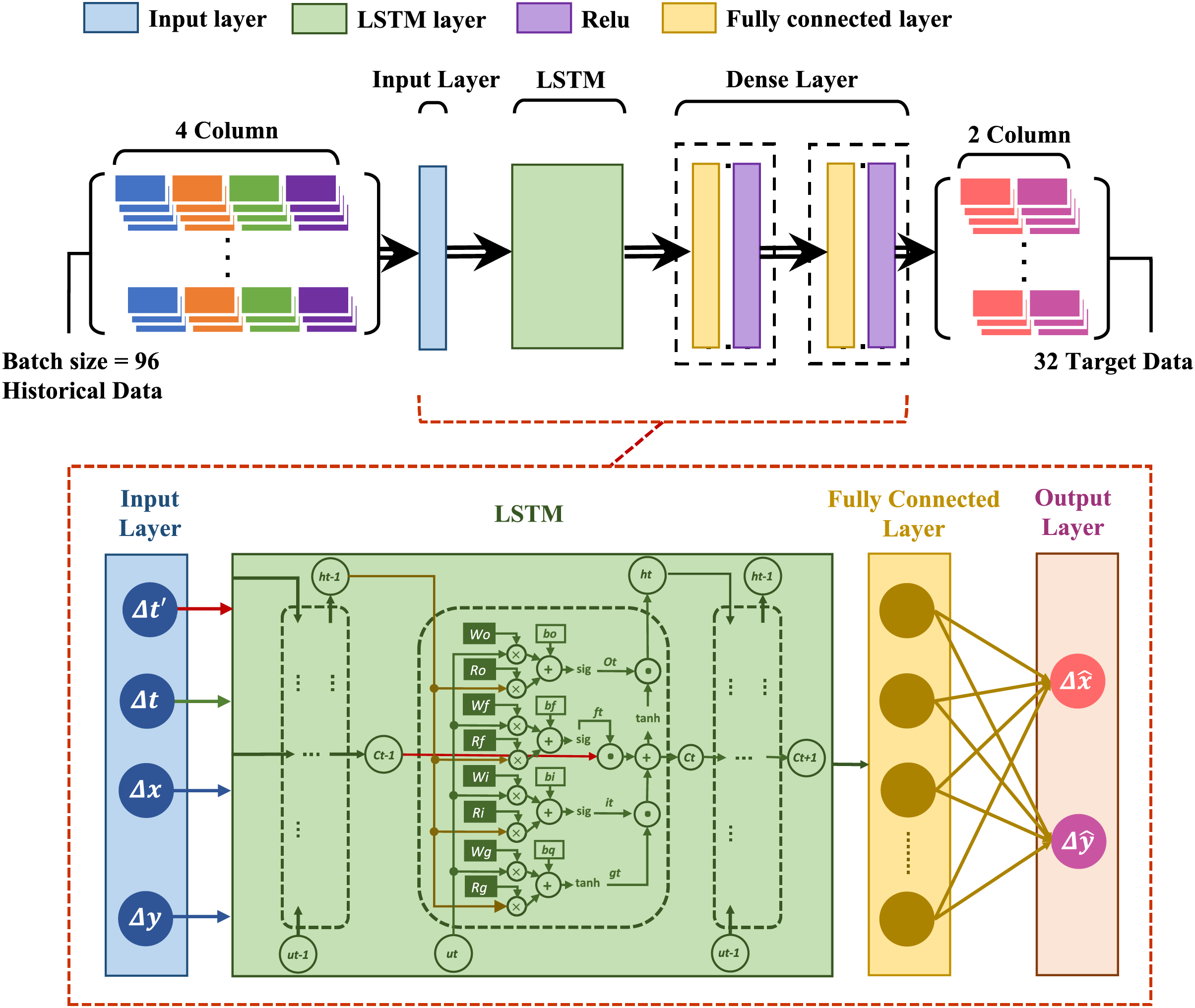
Figure 3: A complete architecture with four input data to LSTM model and final output as latitude and longitude

Δτip(l)=τip(l)−τip(l−1)(8)

Δξip(l)=ξip(l)−ξip(l−1)(9)

Δηip(l)=ηip(l)−ηip(l−1)(10)

For each time step l=1,…,ni−1, with ni representing the length of the i-th path (signifying the total count of path points), the NN receives the input vector:

Δvip(l)=[Δξip(l), Δηip(l), Δτip(l), Δτip(l+1)](11)

To manage variability in trajectory lengths, a standard zero-padding technique [33] is applied. This ensures each trajectory length matches the longest trajectory in the dataset by appending zero-value segments at the start of each trajectory.

To streamline the notation in the LSTM equations, the indices p and i are omitted. Thus, at each time step l, the LSTM unit ingests the input vector Δv(l+1), the preceding cell state c(l), and the prior hidden state h(l). Additionally, An intermediate state c~(l+1) is also generated, representing the candidate state for the memory cells. The LSTM architecture incorporates three gate mechanisms, the forget (f), input (i), and output (o) gates, along with the intermediate state c~, cell state c, and hidden state h, These components undergo updates as follows:

f(l+1)=σ(Wf⋅Δv(l+1)+Uf⋅h(l)+bf)(12)

i(l+1)=σ(Wi⋅Δv(l+1)+Ui⋅h(l)+bi)(13)

o(l+1)=σ(Wo⋅Δv(l+1)+Uo⋅h(l)+bo)(14)

c~(l+1)=tanh⁡(Wc⋅Δv(l+1)+Uc⋅h(l)+bc)(15)

c(l+1)=f(l+1)⊙c(l)+i(l+1)⊙c~(l+1)(16)

h(l+1)=o(l+1)⊙tanh⁡(c(l+1))(17)

where W, U, and b denote the input, recurrent weight matrices, and bias vectors respectively, ⊙ symbolizes the Hadamard product, and tanh⁡(⋅) and σ(⋅) represent the Hyperbolic tangent and sigmoid activation functions, respectively. The LSTM’s outputs then feed into a Fully Connected Layer (FCL) with a rectified linear unit activation function:

ϱ(v)=max(0, v)(18)

In the FCL, each neuron is interconnected with all neurons from the preceding layer, effectuating an operation for neuron n as follows:

n=∑mαmhm+βn(19)

where hm denotes the response of the preceding layer and the m-th input to neuron n, αm is the m-th weight, and β is the bias. Consequently, the FCL’s output is calculated by:

fcl(l+1)=ρ(α(l+1)Th(l+1))(20)

where α(l+1) are the weights of the FCL. The NN’s overall predicted output Δd^(l+1) results from a linear combination of the FCL’s responses fcl(l+1) and the final regression coefficients α^(l+1), as described by:

Δd^(l+1)=α^(l+1)Tfcl(l+1)(21)

The intended outputs of the NN and the framework are detailed as follows:

Δdip(l+1)=[Δξip(l+1), Δηip(l+1)](22)

dip(l+1)=[ξip(l+1), ηip(l+1)](23)

Upon completion of the prediction process, the model forecasts the deviations between successive points, specified as:

Δd^ip(l+1)=[Δξ^ip(l+1), Δη^ip(l+1)](24)

Lastly, Δd^ip(l+1) is transformed into the predicted framework output d^ip(l+1), applying Eqs. (5)–(7) for ξip(l+1) and ηip(l+1):

d^ip(l+1)=[ξ^ip(l+1), η^ip(l+1)](25)

3  Case Study: AIS Dataset Analysis and Vessel Trajectory Prediction

3.1 AIS Dataset Description

The AIS data utilized in this paper was sourced from EHSolution Company in South Korea and remains proprietary, not available for public use. Our research primarily aimed at analyzing vessel movements, so we concentrated on the positional information provided in the data. This extensive dataset, totaling 7.0 terabytes, includes MMSI, time stamps, speed, heading, latitudes, and longitudes, covering a period from January 2020 to December 2020. Given the enormity of the data, our examination was confined to AIS records from 01 February 2020, to 30 April 2020.

3.2 Data Preprocessing

In this research, the raw dataset provided by EH Solution presents a challenge in preprocessing for precise trajectory predictions. Our methodology involves a comprehensive approach to refine the dataset for enhanced predictive accuracy. We implement a collection of statistical strategies to purify the data. Specifically, for each maritime entity, our data refinement routine encompasses the elimination of duplicate records (by discarding entries with identical timestamps or those with temporal discrepancies under one second), the removal of anomalies (by excluding records with velocities exceeding the upper limit vcrit), and the simplification of static records (by omitting entries indicating near-zero movement, i.e., velocities beneath the lower limit vidle). This latter step is essential to ensure that machine learning algorithms do not process static segments of the trajectory data. Trajectories with a sparse distribution of data points, falling below the threshold λthresh, are deemed non-contributory and are consequently removed to align with the objectives of learning algorithms. The Automatic Identification System (AIS) plays a pivotal role in contemporary maritime navigation, offering vital capabilities such as target identification and location marking. Raw AIS data is utilized to create a benchmark dataset and establish a historical matrix of AIS information, represented as:

ZT=[z1, z2,…,zM]T(26)

where M denotes the aggregate count of AIS messages and

zj=[IDj, τj, ϕjT, χj, ωj](27)

with j∈{1, 2,…,M}. Here, IDj, τj, ϕjT, and ωj signify the Maritime Mobile Service Identity (MMSI), the time stamp, geospatial coordinates (longitude and latitude), course over ground (COG), and speed over ground (VOG), respectively. The MMSI uniquely identifies each maritime vessel.

In preprocessing, we discard any data points associated with stationary or inconsistent vessel behavior. A minimal trajectory time span of 1200 s is established, informed by the typical AIS data reception interval, which ranges between 5 to 10 min, with any interval surpassing 20 min being earmarked for subsequent navigational status phases. The trajectory optimization is conducted via a dedicated function, as defined in Algorithm 1, ensuring the exclusion of irrelevant noise from the initial dataset. The refined data, representing vessels in travel, facilitates a smoother trajectory analysis.

The statistical analysis of raw AIS data has indicated potential inaccuracies, as it showed maximum latitude (LAT) and longitude (LON) values of 91.00 and 181, respectively. These values are beyond the geographical limits of the Korean Peninsula, underscoring the raw data’s potential inaccuracies. However, the accuracy improves significantly after preprocessing the data. The normalized values for LAT and LON become 39.97 and 136.8, respectively. These adjusted values are much more consistent with the geographical boundaries of the region, making them highly appropriate for incorporation into deep learning models designed for the Korean Peninsula. This underscores the critical role of data preprocessing in ensuring the accuracy and usability of data for specific regional applications.

4  Discussion

The vessel trajectory datasets undergo a rigorous classification process following comprehensive data preprocessing, utilizing a diverse array of routes and ship experimental datasets. This classification methodology involves a tripartite partitioning of the data into training, validation, and testing subsets. The training subset serves as the foundation for model development, while the validation subset is employed to assess model performance and enhance its generalization capabilities. The test subset is utilized to generate predictions based on an input-output mapping of N to 1, where the status vectors of the initial N time steps function as input sequences, with the subsequent vessel status serving as output vectors. This approach enables the prediction of vessel states N minutes into the future, utilizing the initial trajectory as the input data.

In this study, we systematically classified the experimental data as follows: 70% for the training set, 15% for the validation set, and the remaining 15% for the test set. This partitioning strategy ensures a robust evaluation of the model’s predictive capabilities while maintaining sufficient data for training and validation purposes.

This methodological approach facilitates a comprehensive assessment of the model’s performance across various operational scenarios, thereby enhancing the reliability and applicability of the predictive framework in real-world maritime contexts.

Xstd=x−xminxmax−xmin(28)

where Xstd denotes normalized data, xmin represents the minimum sample value. Following normalization, data are confined to the interval [0, 1]. The neural network’s output, within the [0, 1] interval, is denormalized to the original scale by:

Xscalar=Xstd(xmax−xmin)+xmin(29)

In this analysis, Xscalar denotes the data post-denormalization. To assess the performance of the Gated Recurrent Unit (GRU) in predicting vessel traffic flow, a Long Short-Term Memory (LSTM) model serves as a comparative baseline. The performance evaluation employs two key metrics: Mean Squared Error (MSE) and Mean Absolute Error (MAE). These metrics function as the primary error analysis indices during the model training phase, providing quantitative measures of prediction accuracy and model performance.

MAE=1n∑i=1n|yi−y^i|(30)

MSE=1n∑i=1n(yi−y^i)2(31)

where yi denotes ground-truth trajectory value and y^i denotes predicted value. The selection of parameters plays a crucial role in determining the efficacy of recurrent neural networks. Generally, an increase in the number of hidden layers corresponds to enhanced model performance and learning capacity. For optimization, this study employs the Adam optimizer [34], a method that combines stochastic gradient descent with adaptive learning rate optimization.

The sampling rate is fixed at 1, while two essential hyper-parameters, batch size and the number of neurons are empirically evaluated to determine their optimal combination [35]. The experimental design considers batch sizes of 8, 16, 24, and 32, while the number of neurons is varied among 60, 80, 100, 120, 140, and 160. This systematic approach to hyper-parameter tuning ensures a comprehensive exploration of the model’s parameter space, facilitating the identification of the most effective configuration for the task at hand.

The parameter selection process reveals an inverse relationship between batch size and computation time, with larger batches reducing calculation time proportionally. However, extreme batch sizes lead to increased errors. A comparison of 16 and 24 neuron configurations shows similar computation time, but the 16-neuron setup yields lower error rates, indicating its optimality. As neuron count increases, so does processing time, while prediction errors decrease from 60 to 120 neurons. Beyond 120 neurons, error rates rise. Considering these factors, a configuration of 100 neurons appears to offer an optimal balance between computational efficiency and prediction accuracy.

Based on extensive experimental testing and parameter optimization, the Gated Recurrent Unit (GRU) architecture has been designed with the following structure: a fully connected layer, an activation layer, dual GRU layers, and a dropout mechanism, collectively forming the GRU recurrent neural network. The second and fourth layers, denoted as gru1, and gru2, respectively, represent the GRU layers, each containing 120 hidden units.

The third and fifth layers implement the dropout method, which serves a dual purpose: maintaining model robustness by mitigating information loss during training, and acting as a regularization technique to reduce weight connections. This approach enhances the network’s resilience when specific connection information is absent. The final layer is a fully connected layer comprising two neurons. The architectural representation of this GRU neural network is illustrated in Fig. 4.

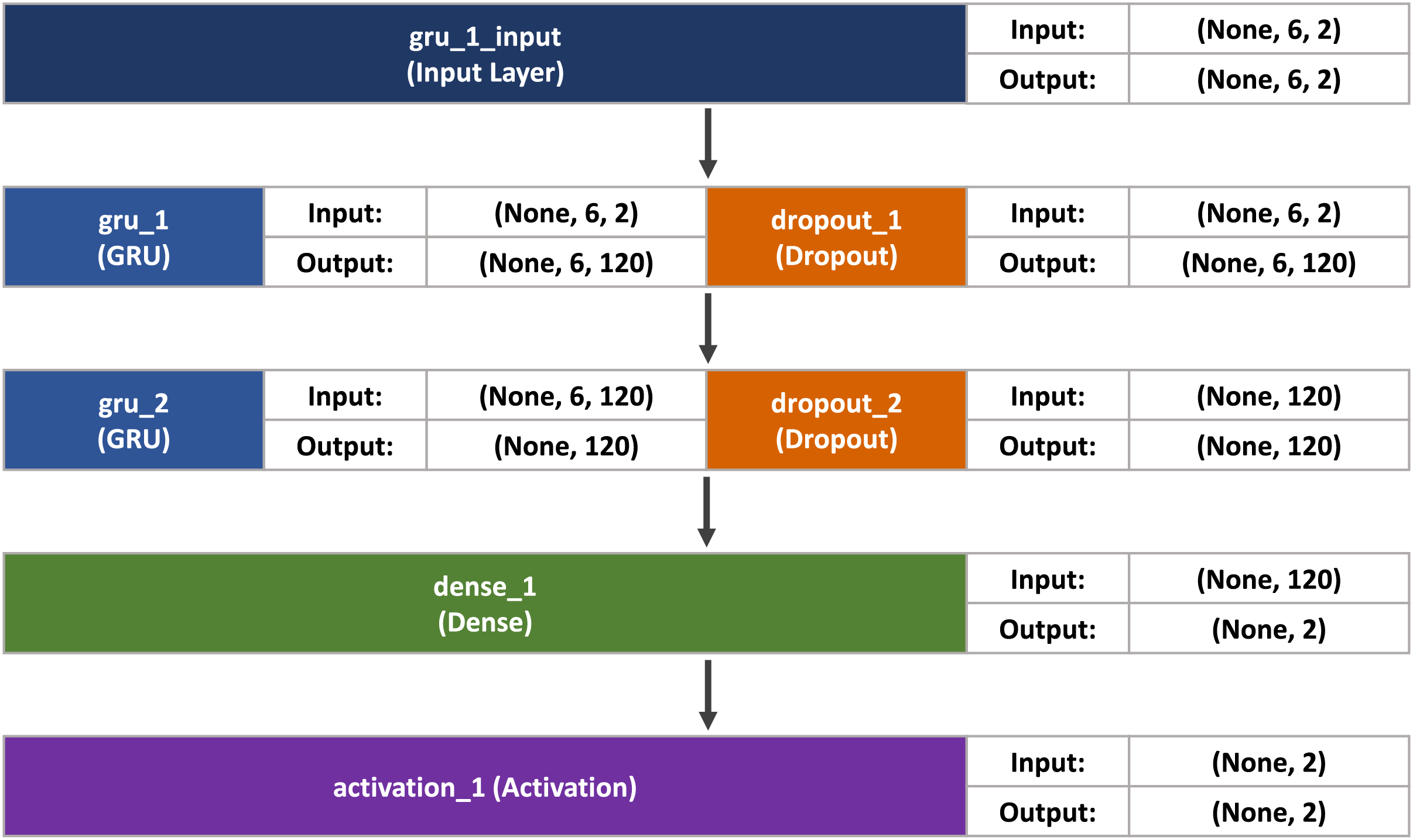
Figure 4: GRU model used in our proposed system

4.1 Experiment on Large Dataset

This experiment involved multiple ship datasets. Notably, the model parameters were personalized to each dataset, reflecting a complex configuration to optimize performance. In our experimental results, the focus is on two key neural network models, namely LSTM and GRU, for trajectory prediction tasks. The aim is to comprehensively evaluate and compare the predictive performance of LSTM and GRU models, seeking to determine the most suitable option for trajectory prediction tasks. The aim is to comprehensively evaluate and compare the predictive performance of LSTM and GRU models, seeking to determine the most suitable option for these tasks. We have proposed an efficient LSTM and GRU based smart vessel trajectory prediction using AIS data. The proposed system takes latitude, longitude, speed, and heading from the AIS dataset and provides them as input to the LSTM and GRU to predict the vessel trajectory. Three months of AIS data have been used to validate the results of our model.

Table 1 presents the performance comparison between LSTM and GRU models for predicting the trajectory of ship ID AXZ-00797, while Fig. 5 presents trajectory predictions. Both models are trained and validated on the AIS dataset, with their respective training and validation losses noted. For the LSTM model, the MSE during training is 0.0156, and during validation, it slightly increases to 0.0159. Similarly, the MAE for training is 0.0815, and for validation, it rises slightly to 0.0834.

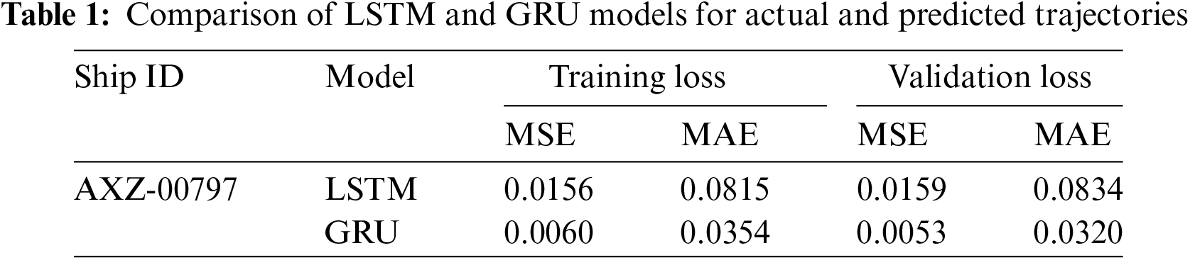
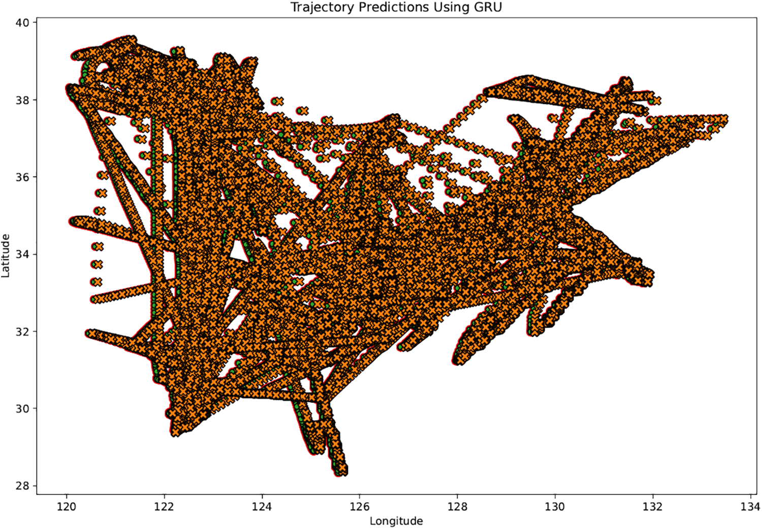
Figure 5: Actual and predicted trajectory prediction model based on LSTM and GRU model. Trajectory plot with the following legends: History, Target, and Predicted. The x-axis represents longitude (°), and the y-axis represents latitude (°)

On the other hand, the GRU model exhibits lower losses across both training and validation. Specifically, it achieves an MSE of 0.0060 during training and 0.0053 during validation. Correspondingly, the MAE for the GRU model is notably lower, with values of 0.0354 for training and 0.0320 for validation. Overall, the results indicate that the GRU model outperforms the LSTM model in predicting the ship’s trajectory, as it consistently demonstrates lower losses for both training and validation datasets. These results demonstrate that the GRU architecture may be more effective in capturing the temporal dependencies and patterns in the trajectory data, leading to more accurate predictions. However, further analysis and experimentation are necessary to understand the underlying reasons for the observed differences in performance between the two models. Fig. 5 shows the comparison of LSTM and GRU models for actual and predicted trajectories.

4.2 Experiments on Small Dataset

This section analyzes the results from experiments on small datasets, comparing the performance of several neural network models and the Kalman Filter. The models tested include LSTM, GRU, DBLSTM, and Simple RNN. These experiments, conducted on datasets associated with various ship IDs, offered a wide range of scenarios to evaluate how well these models performed. Fig. 6 displays sample trajectories obtained from the LSTM and GRU model simulations.

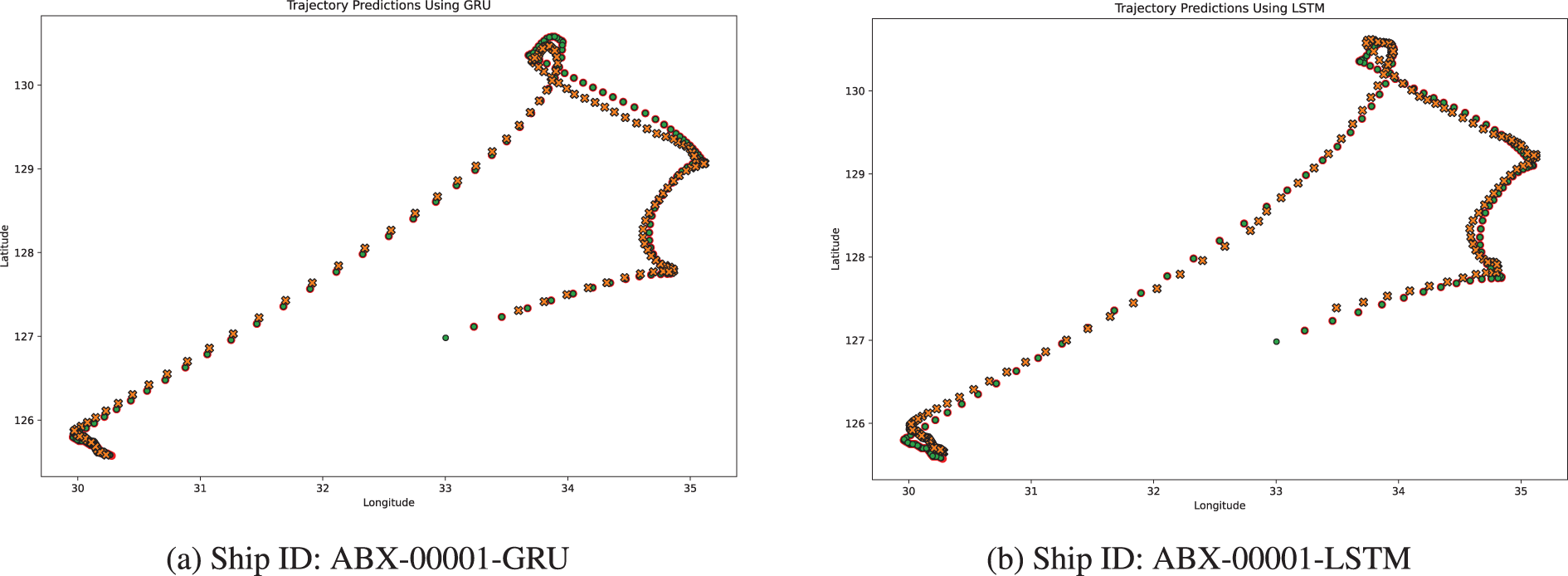
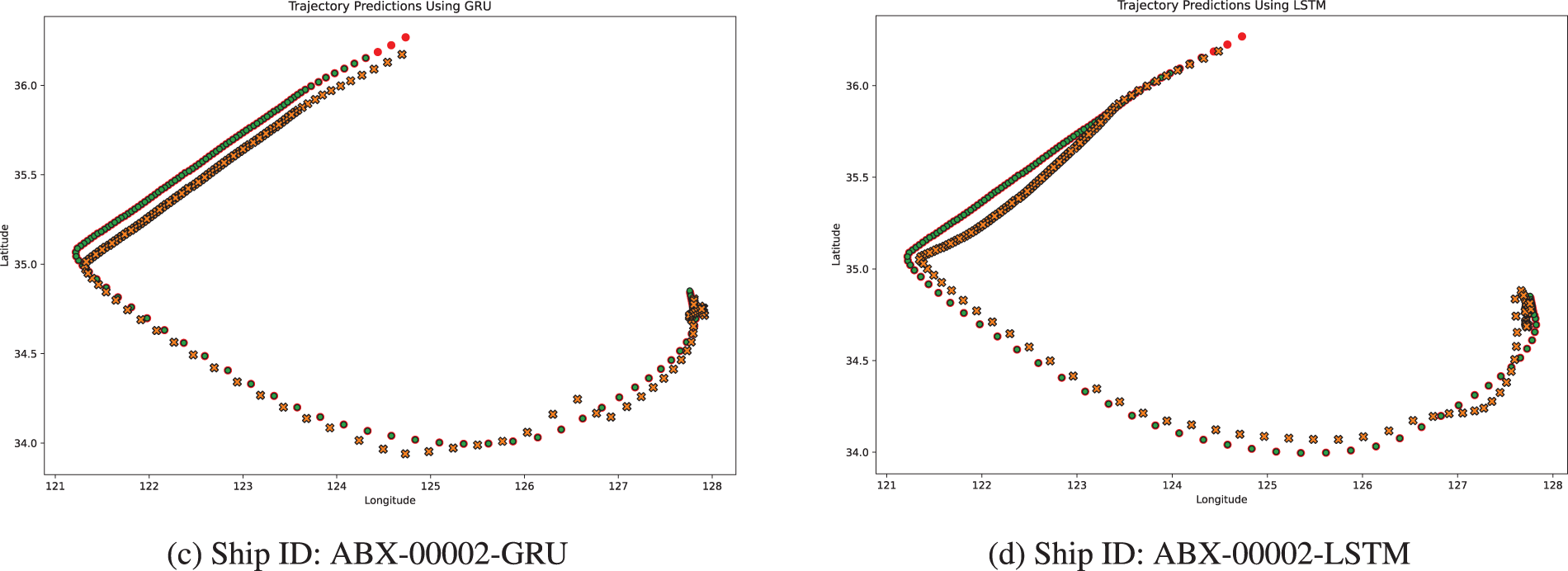
Figure 6: (a–d) show the Actual trajectories vs. predicted trajectories for different ship IDs using GRU and LSTM. Trajectory plot with the following legends: History, Target and Predicted. The x-axis represents longitude (°), and the y-axis represents latitude (°)

The analysis focuses on four key performance metrics: MSE, MAE, ADE, and FDE. These metrics are crucial for assessing model accuracy and reliability, revealing distinct patterns across different models and datasets.

The results presented in Table 2 show that the GRU model consistently demonstrates superior performance across multiple datasets, frequently achieving lower MSE and MAE values compared to other models. This suggests that the GRU is capable of generating more precise predictions with fewer significant errors. For instance, in datasets such as ABX-00001 and ABX-00002, the GRU model outperforms the LSTM and other models in terms of MSE and MAE. Furthermore, the GRU model excels in ADE and FDE, metrics that gauge both average and final prediction accuracy, reinforcing the notion that GRU is particularly effective in modeling time-series data, making it a strong candidate for maritime navigation tasks.

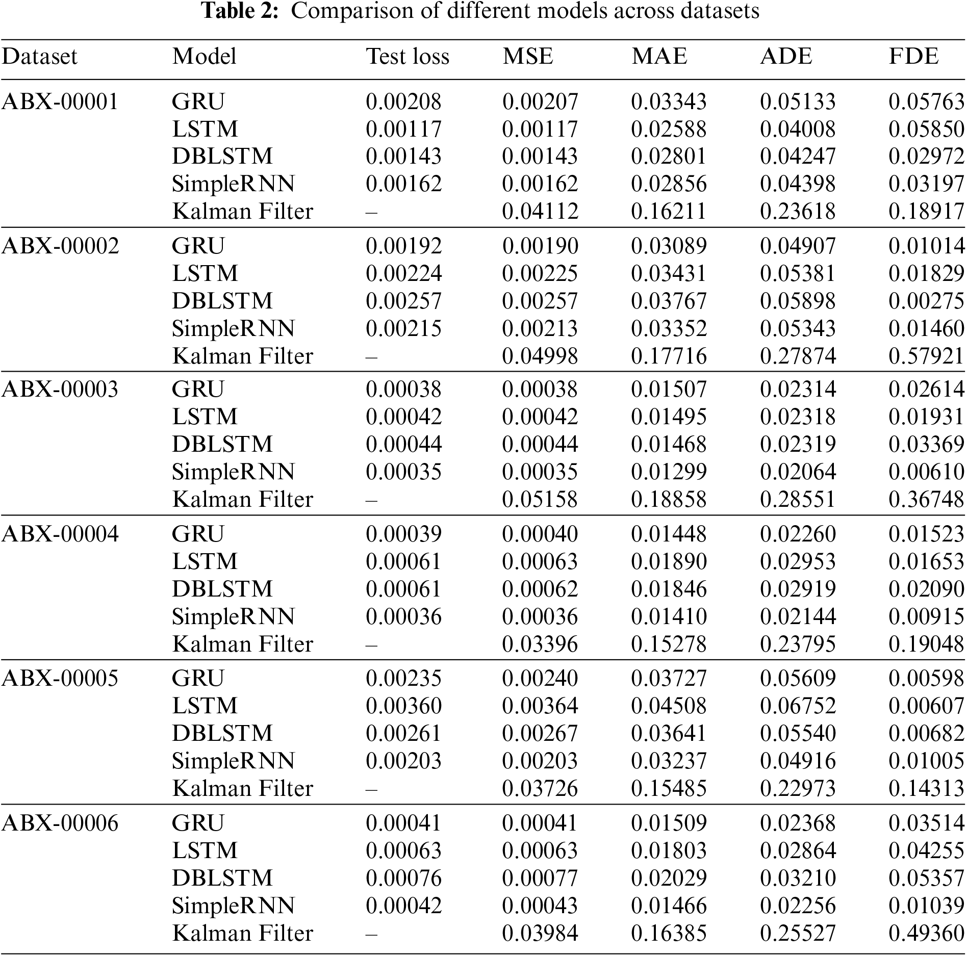
In contrast, while the LSTM model exhibits competitive performance, particularly during the training phases, it generally records higher losses in both MSE and MAE during validation across several ship IDs. For example, in dataset ABX-00001, although the LSTM achieves a lower training loss, it records a slightly higher validation loss compared to the GRU, indicating a potential tendency towards overfitting. A notable exception is observed with Ship ID ABX-00002, where the LSTM model performs better in training MSE than the GRU. However, the GRU exhibits a slight advantage in validation MAE, hinting at superior generalization capabilities.

In some instances, such as with dataset ABX-00003, the DBLSTM records lower MAE but struggles with higher ADE and FDE values. This indicates that while it may reduce average errors, its final predictions can occasionally deviate more significantly from the target.

The SimpleRNN model, characterized by its simpler architecture, tends to record higher errors across all metrics. For example, in dataset ABX-00004, SimpleRNN shows relatively higher MSE and MAE, underscoring its limitations in capturing complex temporal dependencies as effectively as the more advanced models like GRU and LSTM.

The Kalman Filter, included as a baseline non-neural approach, predictably records higher errors across all metrics when compared to the neural network models. Across all datasets, the Kalman Filter exhibits significantly higher MSE, MAE, ADE, and FDE values, highlighting the clear advantages of utilizing deep learning models for time-series prediction tasks within the context of AIS data.

The GRU model is efficient and less demanding on computational resources, making it a good choice for situations with limited computing power, like onboard maritime systems. Its strong performance across different datasets shows it’s ideal for real-time predictions where both accuracy and efficiency are important.

The LSTM model can still be useful when there is plenty of training data available, as it can effectively use its longer memory. The DBLSTM, while not always better than other models, should be explored more for cases where understanding context from both directions is important. Despite its higher error rates, the Kalman Filter remains relevant in contexts where model simplicity and interpretability are prioritized over precision.

Overall, the results suggest that GRUs are particularly advantageous for handling AIS datasets and related problem settings, with their lower losses indicating a reduced likelihood of significant prediction errors as shown in Fig. 7. This makes them a preferable choice for critical applications like maritime navigation and predictive maintenance, where consistent and reliable model performance is essential.

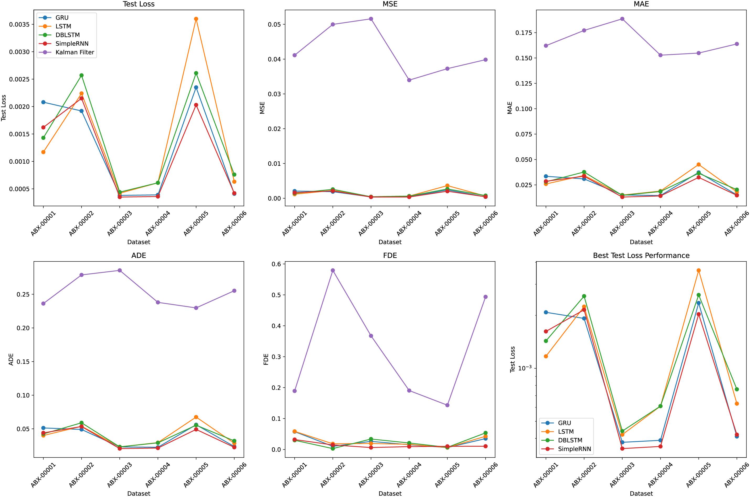
Figure 7: Comparison of actual and predicted trajectory prediction model based on LSTM model

5  Conclusion

This paper evaluates vessel trajectory prediction using advanced neural network models LSTM, GRU, DBLSTM, SimpleRNN, and the Kalman Filter based on three months of AIS data. The GRU model consistently outperforms with lower MSE (0.00208) and MAE (0.03343) compared to LSTM (MSE: 0.00117, MAE: 0.02588), DBLSTM (MSE: 0.00143, MAE: 0.02801), and SimpleRNN (MSE: 0.00162, MAE: 0.02856). In terms of trajectory accuracy, GRU achieves lower Average Displacement Error (ADE) and Final Displacement Error (FDE) across multiple datasets, with values as low as 0.02314 (ADE) and 0.00598 (FDE) in some cases. While LSTM shows strong training performance, its tendency to overfit suggests GRU as a more reliable choice. The DBLSTM, despite its potential, does not consistently surpass GRU, and the SimpleRNN and Kalman Filter, though simpler, lack the accuracy of the more sophisticated models, with the Kalman Filter often showing MSE values above 0.03 and MAE values exceeding 0.15. These results highlight the effectiveness of GRU for real-time maritime applications such as collision avoidance, where both prediction accuracy and computational efficiency are crucial.

While our preprocessing efforts significantly improved data quality, the study was constrained by the dataset’s limited size and proprietary nature. Future research will explore integrating GRU with encoder-decoder architectures and federated learning techniques, allowing multi-horizon predictions and combining data from multiple ships. We also aim to develop hybrid approaches that merge deep learning with traditional methods, investigate transfer learning, real-time implementations, and incorporate environmental data to enhance model accuracy and applicability. Additionally, improving model explainability will be crucial for its practical adoption by maritime professionals.

Acknowledgement: This study was partly supported by the “Regional Innovation Strategy (RIS)” through the National Research Foundation of Korea (NRF) funded by the Ministry of Education (MOE) (2021RIS-004) and an Institute of Information and Communications Technology Planning and Evaluation (IITP) grant funded by the Korean government (MSIT) (No. RS-2022-00155857, Artificial Intelligence Convergence Innovation Human Resources Development (Chungnam National University)).

Funding Statement: This study was funded by the “Regional Innovation Strategy (RIS)” through the National Research Foundation of Korea (NRF) funded by the Ministry of Education (MOE) (2021RIS-004) and an Institute of Information and Communications Technology Planning and Evaluation (IITP) grant funded by the Korean government (MSIT) (No. RS-2022-00155857, Artificial Intelligence Convergence Innovation Human Resources Development (Chungnam National University)).

Author Contributions: Conceptualization: Umar Zaman, Junaid Khan, and Kyungsup Kim; Methodology: Umar Zaman, Junaid Khan, Eunkyu Lee, and Sajjad Hussain; Software: Umar Zaman, and Junaid Khan; Validation: Umar Zaman, Junaid Khan, Sajjad Hussain, Awatef Salim Balobaid, and Rua Yahya Aburasain; Formal Analysis: Umar Zaman, Junaid Khan, and Sajjad Hussain; Investigation: Umar Zaman and Junaid Khan; Writing—Original Draft Preparation: Umar Zaman, Junaid Khan, and Sajjad Hussain; Writing—Review and Editing: Umar Zaman, Junaid Khan, Eunkyu Lee, Awatef Salim Balobaid, and Umar Zaman; Visualization: Umar Zaman, and Junaid Khan; Supervision: Kyungsup Kim; Project Administration: Kyungsup Kim; Funding Acquisition: Kyungsup Kim. All authors reviewed the results and approved the final version of the manuscript.

Availability of Data and Materials: Data can be obtained by contacting sclkim@cnu.ac.kr.

Ethics Approval: Not applicable. This studies not involving humans or animals.

Conflicts of Interest: The authors declare that they have no conflicts of interest to report regarding the present study.

References

1. L. Frković, B. Ćosić, T. Pukšec, and N. Vladimir, “Vehicle-to-ship: Enhancing the energy transition of maritime transport with the synergy of all-electric vehicles and ferries,” IEEE Trans. Transp. Electr., vol. 10, no. 3, pp. 6010–6023, 2023. doi: 10.1109/TTE.2023.10111234. [Google Scholar] [CrossRef]

2. A. Miglani and N. Kumar, “Deep learning models for traffic flow prediction in autonomous vehicles: A review, solutions, and challenges,” Veh. Commun., vol. 20, 2019, Art. no. 100184. doi: 10.1016/j.vehcom.2019.100184. [Google Scholar] [CrossRef]

3. L. P. Perera, P. Oliveira, and C. G. Soares, “Maritime traffic monitoring based on vessel detection, tracking, state estimation, and trajectory prediction,” IEEE Trans. Intell. Transp. Syst., vol. 13, no. 3, pp. 1188–1200, 2012. doi: 10.1109/TITS.2012.2187282. [Google Scholar] [CrossRef]

4. E. Lee, J. Khan, W. J. Son, and K. Kim, “An efficient feature augmentation and LSTM-based method to predict maritime traffic conditions,” Appl. Sci., vol. 13, no. 4, 2023, Art. no. 2556. doi: 10.3390/app13042556. [Google Scholar] [CrossRef]

5. P. Borkowski, “The ship movement trajectory prediction algorithm using navigational data fusion,” Sensors, vol. 17, no. 6, 2017, Art. no. 1432. doi: 10.3390/s17061432. [Google Scholar] [PubMed] [CrossRef]

6. R. W. Liu, J. Nie, S. Garg, Z. Xiong, Y. Zhang and M. S. Hossain, “Data-driven trajectory quality improvement for promoting intelligent vessel traffic services in 6G-enabled maritime IoT systems,” IEEE Internet Things J., vol. 8, no. 7, pp. 5374–5385, 2020. doi: 10.1109/JIOT.2020.3028743. [Google Scholar] [CrossRef]

7. E. Lee, J. Khan, U. Zaman, J. Ku, S. Kim and K. Kim, “Synthetic maritime traffic generation system for performance verification of maritime autonomous surface ships,” Appl. Sci., vol. 14, no. 3, 2024, Art. no. 1176. doi: 10.3390/app14031176. [Google Scholar] [CrossRef]

8. Y. Liu, J. Liu, Q. Zhang, Y. Liu, and Y. Wang, “Effect of dynamic safety distance of heterogeneous traffic flows on ship traffic efficiency: A prediction and simulation approach,” Ocean Eng., vol. 294, 2024, Art. no. 116660. doi: 10.1016/j.oceaneng.2023.116660. [Google Scholar] [CrossRef]

9. E. Tu, G. Zhang, L. Rachmawati, E. Rajabally, and G. B. Huang, “Exploiting ais data for intelligent maritime navigation: A comprehensive survey from data to methodology,” IEEE Trans. Intell. Transp. Syst., vol. 19, no. 5, pp. 1559–1582, 2017. doi: 10.1109/TITS.2017.2724551. [Google Scholar] [CrossRef]

10. D. Caveney, “Numerical integration for future vehicle path prediction,” in 2007 Am. Control Conf., New York, NY, USA, Jul. 2007, pp. 3906–3912. [Google Scholar]

11. H. Li, J. Liu, Z. Yang, R. W. Liu, K. Wu and Y. Wan, “Adaptively constrained dynamic time warping for time series classification and clustering,” Inf. Sci., vol. 534, pp. 97–116, 2020. doi: 10.1016/j.ins.2020.04.009. [Google Scholar] [CrossRef]

12. Z. L. Ouyang, G. Chen, and Z. J. Zou, “Identification modeling of ship maneuvering motion based on local gaussian process regression,” Ocean Eng., vol. 267, 2023, Art. no. 113251. doi: 10.1016/j.oceaneng.2022.113251. [Google Scholar] [CrossRef]

13. Y. Meng, X. Zhang, and X. Zhang, “Identification modeling of ship nonlinear motion based on nonlinear innovation,” Ocean Eng., vol. 268, 2023, Art. no. 113471. doi: 10.1016/j.oceaneng.2022.113471. [Google Scholar] [CrossRef]

14. D. D. Nguyen, C. L. Van, and M. I. Ali, “Vessel trajectory prediction using sequence-to-sequence models over spatial grid,” in Proc. 12th ACM Int. Conf. Distrib. Event-Based Syst., Hamilton, New Zealand, Jun. 2018, pp. 258–261. [Google Scholar]

15. L. Cao, Y. Luo, Y. Wang, J. Chen, and Y. He, “Vehicle sideslip trajectory prediction based on time-series analysis and multi-physical model fusion,” J. Intell. Connected Veh., vol. 6, pp. 161–172, 2023. doi: 10.26599/JICV.2023.9210016. [Google Scholar] [CrossRef]

16. B. Zhang, W. Yu, Y. Jia, D. Yang J.Huang, and Z. Zhong, “Predicting vehicle trajectory via combination of model-based and data-drivenmethods usingKalman filter,” Proc. Inst. Mech, Eng. Part D: J. Automobile Eng., vol. 238, no. 8, pp. 2437–2450, 2023. doi: 10.1177/09544070231161846. [Google Scholar] [CrossRef]

17. Y. Zheng, “Trajectory data mining: An overview,” ACM Trans. Intell. Syst. Technol., vol. 6, no. 3, pp. 1–41, 2015. doi: 10.1145/2743025. [Google Scholar] [CrossRef]

18. G. Siegert, P. Banyś, C. S. Martínez, and F. Heymann, “EKF based trajectory tracking and integrity monitoring of AIS data,” in 2016 IEEE/ION Position, Location Navig. Symp. (PLANS), Savannah, GA, USA, Apr. 2016, pp. 887–897. [Google Scholar]

19. J. P. Llerena, J. García, and J. M. Molina, “LSTM vs. CNN in real ship trajectory classification,” in Int. Workshop Soft Comput. Models Ind. Environ. Appl., 2021, pp. 58–67. [Google Scholar]

20. L. You et al., “ST-Seq2Seq: A spatio-temporal feature-optimized Seq2Seq model for short-term vessel trajectory prediction,” IEEE Access, vol. 8, pp. 218565–218574, 2020. doi: 10.1109/ACCESS.2020.3041762. [Google Scholar] [CrossRef]

21. Z. Chen, Z. Ding, D. J. Crandall, and L. Liu, “Polyline generative navigable space segmentation for autonomous visual navigation,” IEEE Robot. Autom. Lett., vol. 8, no. 4, pp. 2054–2061, 2023. doi: 10.1109/LRA.2023.3246383. [Google Scholar] [CrossRef]

22. B. Ivanovic, K. Leung, E. Schmerling, and M. Pavone, “Multimodal deep generative models for trajectory prediction: A conditional variational autoencoder approach,” IEEE Robot. Autom. Lett., vol. 6, no. 2, pp. 295–302, 2020. doi: 10.1109/LRA.2020.3043163. [Google Scholar] [CrossRef]

23. X. Chen, J. Xu, R. Zhou, W. Chen, J. Fang and C. Liu, “TrajVAE: A variational autoencoder model for trajectory generation,” Neurocomputing, vol. 428, pp. 332–339, 2021. doi: 10.1016/j.neucom.2020.03.120. [Google Scholar] [CrossRef]

24. A. D. Leege, M. Van Paassen, and M. Mulder, “A machine learning approach to trajectory prediction,” in AIAA Guid., Navig., Control (GNC) Conf., Boston, MA, USA, Aug. 2013, p. 4782. [Google Scholar]

25. J. Khan, E. Lee, and K. Kim, “A higher prediction accuracy-based alpha-beta filter algorithm using the feedforward artificial neural network,” CAAI Trans. Intell. Technol., vol. 8, no. 4, pp. 1124–1139, 2023. doi: 10.1049/cit2.12148. [Google Scholar] [CrossRef]

26. J. Khan, E. Lee, and K. Kim, “Optimizing the performance of Kalman filter and alpha-beta filter algorithms through neural network,” in 2023 9th Int. Conf. Control, Decis. Inform. Technol. (CoDIT), Istanbul, Turkey, May 2023, pp. 2187–2192. [Google Scholar]

27. M. J. Kaiser and S. Narra, “Application of AIS data in service vessel activity description in the gulf of Mexico,” Maritime Econ. Logist., vol. 16, pp. 436–466, 2014. doi: 10.1057/mel.2014.25. [Google Scholar] [CrossRef]

28. Y. A. Ahmed and K. Hasegawa, “Implementation of automatic ship berthing using artificial neural network for free running experiment,” IFAC Proc. Vol., vol. 46, no. 33, pp. 25–30, 2013. doi: 10.3182/20130918-4-JP-3022.00036. [Google Scholar] [CrossRef]

29. D. Zissis, E. K. Xidias, and D. Lekkas, “Real-time vessel behavior prediction,” Evol. Syst., vol. 7, pp. 29–40, 2016. doi: 10.1007/s12530-015-9133-5. [Google Scholar] [CrossRef]

30. S. Hochreiter and J. Schmidhuber, “Long short-term memory,” Neural Comput., vol. 9, no. 8, pp. 1735–1780, 1997. doi: 10.1162/neco.1997.9.8.1735. [Google Scholar] [PubMed] [CrossRef]

31. J. Chung, C. Gulcehre, K. Cho, and Y. Bengio, “Empirical evaluation of gated recurrent neural networks on sequence modeling,” 2014, arXiv:1412.3555. [Google Scholar]

32. A. Graves and J. Schmidhuber, “Framewise phoneme classification with bidirectional LSTM and other neural network architectures,” Neural Netw., vol. 18, no. 5–6, pp. 602–610, 2005. doi: 10.1016/j.neunet.2005.06.042. [Google Scholar] [PubMed] [CrossRef]

33. Z. Zheng, Y. Yang, J. Liu, H. N. Dai, and Y. Zhang, “Deep and embedded learning approach for traffic flow prediction in urban informatics,” IEEE Trans. Intell. Transp. Syst., vol. 20, no. 10, pp. 3927–3939, 2019. doi: 10.1109/TITS.2019.2909904. [Google Scholar] [CrossRef]

34. D. P. Kingma and J. Ba, “Adam: A method for stochastic optimization,” 2014, arXiv:1412.6980. [Google Scholar]

35. J. Yu and M. S. Yang, “Optimality test for generalized FCM and its application to parameter selection,” IEEE Trans. Fuzzy Syst., vol. 13, no. 1, pp. 164–176, 2005. doi: 10.1109/TFUZZ.2004.836065. [Google Scholar] [CrossRef]