Demand-Responsive Transportation Vehicle Routing Optimization Based on Two-Stage Method

1  Introduction

Rapid urbanization in China and evolving travel demands challenge traditional public transportation’s adaptability [1]. The current public transportation system falls short of addressing the increasingly varied transportation needs, particularly in high-density urban areas. While traditional transportation methods meet most travelers’ needs, their low reliability and service levels deter many passengers [2]. Additionally, traditional bus systems typically operate on fixed routes and schedules, lacking the flexibility to adjust routes and timings based on passenger demand or traffic conditions. Moreover, traditional buses have limited passenger capacity and service coverage, which can lead to overcrowding during peak hours, increased waiting times for passengers, and an inability to meet the demands of certain areas or specific time periods [3]. Urban residents mainly travel short to medium distances. Taxis offer flexibility but limited capacity, whereas subways provide high capacity but lack flexibility. Urban public transportation systems, in contrast, offer wide coverage, large capacity, and high flexibility [4]. Therefore, integrating existing urban public transportation systems with passenger demands, allowing for flexible stops and routes, is essential for adaptability. Demand-Responsive Transportation (DRT) offers flexible public transportation, providing passengers with similar travel needs (origin, destination, and times) with direct, punctual, and reliable services based on their requests. DRT has emerged as a promising sustainable solution to meet travelers’ diverse and personalized needs [5–7].

Demand-Responsive Transportation (DRT) provides convenient, eco-friendly, and comfortable services for people sharing similar departure points, destinations, and travel times [8]. Research indicates that flexible bus services can significantly decrease private car usage [9,10]. Additionally, DRT can alleviate urban traffic congestion [11]. Well-planned routes are crucial for effective DRT operation. Optimal DRT route selection reduces passenger travel costs and time, improves DRT companies’ economic efficiency, lowers carbon emissions, and benefits the environment.

Extensive research has been conducted on demand-responsive buses. However, most studies focus on DRT vehicle scheduling [12,13], benefits for enterprises and passengers [14–17], market adaptability [18,19], fare systems [20–23], travel mode selection characteristics [24–26], travel in night scenes [27]. Most studies primarily consider the interests of operators and passengers, overlooking social benefits like CO2 emissions. Additionally, there is limited research on route optimization for DRT buses. Route optimization is essential for DRT systems, directly impacting operational costs and passenger experience. Effective route optimization can significantly reduce empty mileage and fuel consumption, lowering operational costs. It also shortens passenger waiting and travel times, enhancing service quality and satisfaction. Conversely, poor route planning can cause traffic congestion and environmental pollution, negatively impacting society and the environment. Thus, exploring a scientific and practical method for DRT route optimization is both urgent and crucial.

Meanwhile, specific optimization of DRT routes faces many challenges. Firstly, China lacks systematic standards, scientific theories, and methods for DRT route optimization. Secondly, the traditional two-stage method used for multi-demand responsive bus parking and multi-route optimization often compromises the global optimal solution [28,29]. Additionally, DRT route optimization models often mix boarding and alighting stops within one area. In reality, DRT stops have separate boarding and alighting zones on opposite sides of the road, necessitating a division of the network, which is inconsistent with actual conditions [30–33]. More importantly, current route optimization primarily focuses on initial optimization, neglecting real-time passenger demands. As DRT routes are usually predetermined, buses must strictly follow these routes after receiving passenger requests. DRT buses do not accommodate newly added passenger requests, leading to cumulative processing delays. This raises operational costs for DRT operators, fails to address users’ real-time travel needs, and lowers passenger satisfaction [34–38].

Considering these issues, addressing real-time DRT route optimization with random user demands and time windows, and ensuring immediate response to passenger requests within a certain range is crucial for route optimization. Although the core concept of demand-responsive bus route optimization using multi-objective optimization models has been widely explored in previous studies, the two-stage approach proposed in this paper offers a novel method for handling real-time requests. By incorporating both initial and real-time scheduling, this approach ensures a more efficient and responsive transit system. This paper proposes a multi-objective DRT service model that balances benefits for passengers, operators, and carbon emission reductions. Furthermore, an improved NSGA-II genetic algorithm is proposed to address the multi-objective optimization problem of DRT routes.

The structure of this paper includes: The first section discusses relevant literature and makes existing issues summarized. The second section describes and constructs the multi-objective optimization model for demand-responsive bus routes. The third section presents the solution method using an improved NSGA-II genetic algorithm. The fourth section conducts a case study and comparative analysis. Finally, the paper concludes with a summary and discusses potential future research directions.

2  Construction of DRT Bus Route Optimization Model

2.1 Problem Discussion and Model Development

The proposed immediate demand-responsive bus route optimization combines initial and real-time bus requests. The initial request refers to passenger travel requests received before the bus departs. Real-time requests are passenger travel requests received randomly after the vehicle has left the parking area but before it exits the boarding area. In the first stage, passenger time windows are strict, allowing no deviation from scheduled departure or arrival times. The scheduling system, based on pre-booked passenger demands, creates an initial optimized route, which the bus follows to pick up and drop off passengers. In the second stage, passenger time windows are soft, allowing some deviation but with penalties for deviations. The system assesses real-time demands, vehicle position, capacity, and other factors to update the route. If a new demand arises, it is inserted appropriately, updating the route optimized in the first stage. Fig. 1 illustrates the problem within a road network, consisting of two distinct areas: the boarding area and the alighting area, which do not overlap. The network features four bus stops, represented as sectors and named Bus Stop 1 and Bus Stop 2. Initial travel demands create five boarding stops (numbered 1–5) and five alighting stops (numbered 1–5), depicted by orange ovals and squares. As new travel requests arise between departure and the vehicle leaving the boarding area, updated stops emerge, consisting of four new boarding stops (numbered 6–9) and four new alighting stops (numbered 6–9). An effective demand-responsive bus route optimization scheme must accommodate passenger demands at all boarding and alighting stops, including both initial and real-time requests. The uncertain number of passenger requests results in variable numbers of stops, adding to the problem’s complexity. Fig. 1 encompasses four demand-responsive stops, nine boarding stops, and nine alighting stops. The ever-increasing passenger demand poses a significant challenge to route optimization planning, making it essential to develop a more efficient real-time DRT route optimization method. The connections in Fig. 1 illustrate the relationships between nodes; despite map limitations, it is assumed that all nodes are interconnected for this study.

Figure 1: Road network diagram

2.2 Model Assumptions

To facilitate modeling and solving, the following assumptions are made:

(1)   Passenger demand at any stop within the service area is random, with real-time travel requests following a normal distribution.

(2)   Demand-responsive buses travel at a constant speed in the network, disregarding other influencing factors.

(3)   It is known that the distance between all pairs of nodes in the network is determined.

(4)   All initial and real-time passenger demands are within the service area, and each demand is met only once. There are sufficient demand-responsive buses to meet all travel demands.

(5)   The number of passengers with initial demands in the first stage is less than the bus’s seating capacity, and the remaining seats are sufficient for passengers with real-time demands.

(6)   Specify a typical passenger load factor (α=0.9) for the first stage. This assumption ensures a high utilization rate and operational efficiency in the initial scheduling phase.

(7)   Demand-responsive buses can serve multiple stops in a single operation. Although buses maybe go through the stop that has been served many times, every stop can’t be served again.

(8)   Buses cannot travel in reverse.

(9)   Boarding stops and alighting stops do not overlap, nor do boarding and alighting areas.

(10) The distances between stops are based on physical distances and are all known.

(11) All demand can be served within the service area.

2.3 Symbol Definitions

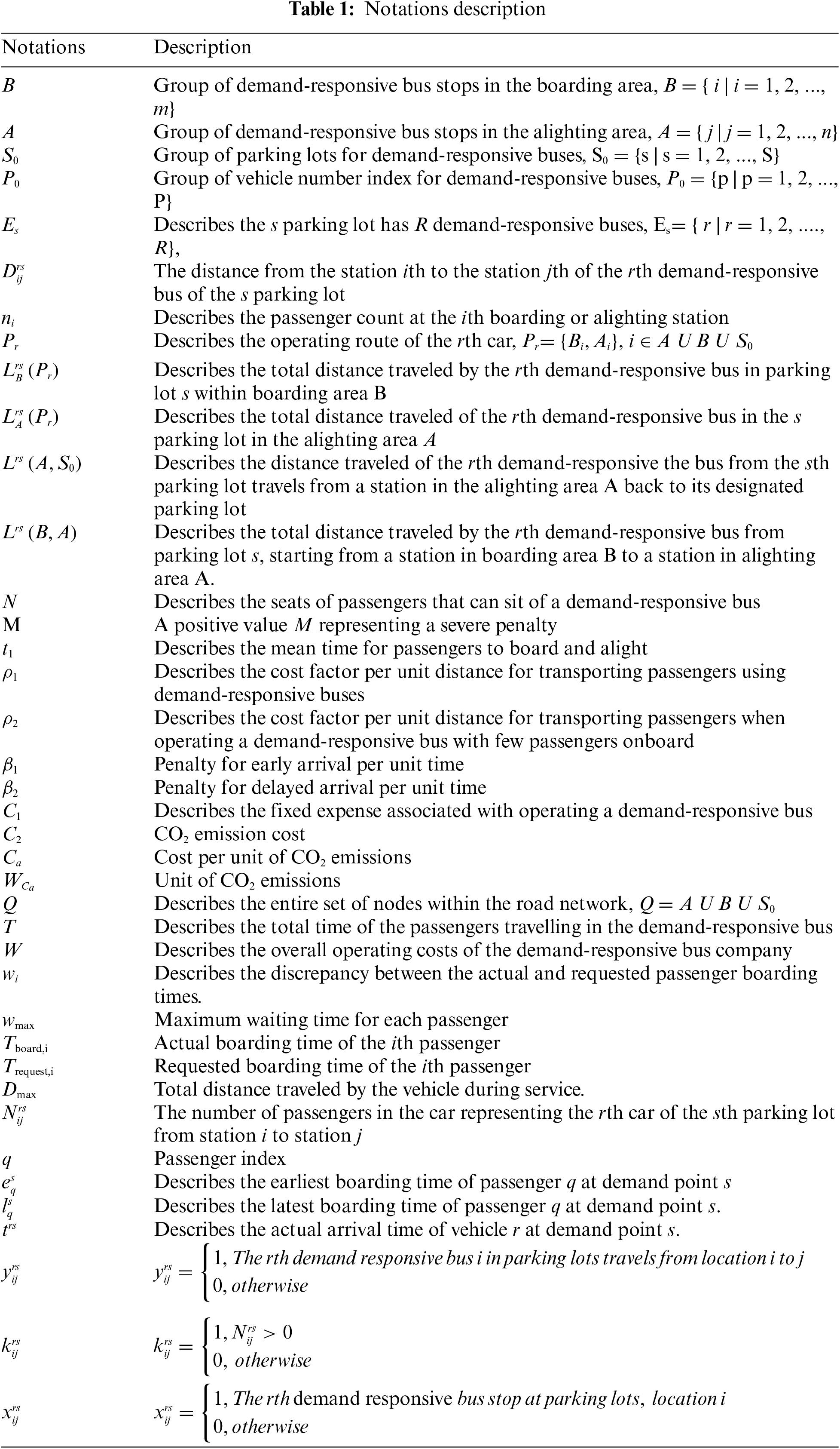
The symbols used in the model formulas and their descriptions are shown in Table 1.

2.4 Real-Time Demand-Responsive Bus Route Multi-Objective Optimization Model Based on Two-Stage

The bus route for multi-objective optimization model is divided into two stages to manage initial and real-time travel requests. The first stage generates a demand-responsive bus route based on requests made before departure. The second stage updates this route in real-time based on new requests. Since both stages share consistent optimization objectives, the model is unified. The road network is divided into boarding and alighting areas. The operation process of the demand-responsive bus involves four components: affiliated bus station, boarding area stop, alighting area stop, and nearest bus station.

Eq. (1) shows the total distance covered by the demand-responsive bus throughout its whole travel.

L=∑s∈S0∑r∈Pr(LBrs(Pr)+Lrs(B,A)+LArs(Ar)+Lrs(A,S0))(1)

There are two objectives to achieve for the route improvement.

Objective 1: Minimize the total travel time for all passengers in the road network. By analyzing the entire travel process of passengers, travel time includes waiting time, boarding and alighting time, and time spent on the bus. Due to the high uncertainty of waiting time, influenced by various factors, the model considers only the time passengers spend on the bus and the boarding and alighting times. First, the time taken by passengers to leave from their starting point to the boarding stop is uncertain. Second, the arrival times of passengers and the demand-responsive bus are uncertain.

The first part is the time passengers spend on the bus, which equals the vehicle’s travel time. Assuming a constant vehicle speed, this time is calculated by dividing the travel distance by the speed. Eq. (2) represents the time spent on the bus. Therefore, the overall travel time includes only the time passengers spend on the bus and the boarding and alighting times.

T1=∑s∈S0∑r∈Pr(∑i∈AUB∑j∈AUBUS0Dijrsyijrs)v(2)

The second part is the passenger boarding and alighting time. The second factor is passenger boarding and alighting time. Individual differences cause these times to vary and be unpredictable. Additionally, as the number of passengers increases, boarding and alighting times extend significantly, making it difficult to quantify exact times for each passenger. To simplify the study, this paper considers boarding and alighting times as fixed averages. The results, based on a field survey of local bus passengers, suggest an average boarding and alighting time of 3 s (t1 = 3 s) [39]. Thus, this model considers only the time passengers spend on the bus and the boarding and alighting times for total travel time in Eq. (3).

T2=∑s∈S0∑r∈Pr∑i∈A∪Bt1nixirs(3)

The objective function, comprising these two parts, is expressed in Eq. (4).

minT=T1+T2(4)

Objective 2: Minimize the whole operational expense of the demand-responsive bus corporation. The operational costs of a demand-responsive bus company include fixed and variable costs. Fixed costs include vehicle purchase, depreciation, and driver wages. Variable costs encompass passenger-related and vehicle-related costs. In practice, fuel consumption and travel distance directly impact CO2 emissions; hence, CO2 emission costs are part of vehicle variable costs.

Calculation of CO2 emission costs in Eq. (5).

C2=CaWCa(∑s∈S0∑r∈Pr∑i∈Q∑j∈QDijrs−∑s∈S0∑r∈Pr∑i∈Q∑j∈QNijrs)(5)

Therefore, minimizing the whole operational expense of the bus corporation is represented in Eq. (6).

minW=∑s∈S0∑r∈Pr∑i∈Q∑j∈Q(ρ1yijrsDijrskijrs+ρ2yijrsDijrs(1−kijrs))+C1+C2(6)

Alighting Constraint: The demand-responsive bus must adhere to the constraint in Eq. (7) when traveling from any boarding stop to an alighting stop.

∑s∈S0∑r∈Pr∑i∈B∑j∈Ayijrs=1,∀i,∀j(7)

Parking Constraint: The bus must satisfy Eq. (8) when departing from a site in the alighting area to its adjacent parking lot.

∑s∈S0∑r∈PR∑i∈A∑j∈S0yijrs=1,∀i,∀j(8)

Demand Constraint: Eq. (9) ensures that the whole travel demand in the roadway system remains within the available supply limits by the buses. This means the number of passengers should be less than the aggregate number of available seats on all demand-responsive buses.

∑i∈Ani≤RSN(9)

Vehicle Capacity Constraint: The number of passengers on each demand-responsive buses must operate within their capacity limits, as shown in Eq. (10). Eq. (10) represents the passenger capacity limit for each bus.

∑s∈S0∑r∈Ps∑i∈Axirsni<Q,∀Pr(10)

Passenger Waiting Time Constraint: The waiting time for each passenger must not exceed the specified maximum, as shown in Eq. (11).

wi≤wmax(11)

Calculation of Passenger Waiting Time:

wi=Tboard,i−Trequest,i(12)

Vehicle Travel Distance Constraint: The total travel distance for each bus must not exceed its maximum, as shown in Eq. (13).

Dmax≤∑s∈S0∑r∈Pr∑i∈Q∑j∈QDijrs(13)

Initial Time Window Constraint: The time window for initial passengers is strict, requiring the vehicle to arrive within the passenger’s requested boarding time window. Failure to do so incurs a high penalty cost.

f1(t)={0eqs≤trs≤lqsMtrs<eqs,trs>lqs(14)

Real-time Time Window Constraint: During real-time scheduling, inserting a new request into the existing route must meet the strict time window constraints of current passengers and those yet to alight. If the time window for real-time demands is also strict, meeting all conditions simultaneously becomes difficult. Hence, during the real-time demand phase, the passenger time window is considered a soft constraint. Typically, the penalty cost per unit for late arrival is higher than for early arrival.

f2(t)={β1(eqs−trs)trs<eqs0eqs≤trs≤lqsβ2(trs−lqs)trs>lqs(15)

This paper presents a two-stage real-time demand-responsive bus route optimization model for managing all demands in the roadway system. Both stages share consistent objectives and models, with the difference lying in the handling of initial and real-time requests.

3  Solution

3.1 Model Feature Analysis

The process is divided into pre-departure and post-departure stages, resulting in a multi-objective optimization model. Analysis reveals two main goals: minimizing total travel time for passengers and reducing operational costs for the bus company, making this a multi-objective problem. Typically, sub-objectives in such optimization conflict, leading to a set of optimal solutions known as Pareto solutions or non-dominated solutions, unlike single-objective optimization which yields a unique approach.

The two objectives presented in this paper are independent and cannot occur simultaneously. Reducing passenger travel time involves more demand-responsive buses, increasing operational costs. Conversely, reducing operational costs requires fewer buses, increasing passenger travel time due to more stops per bus. Balancing these conflicting interests is essential.

Therefore, this paper must balance both interests. A single-objective genetic algorithm cannot achieve this balance. While various multi-objective optimization techniques are available, such as Pareto Simulated Annealing (PSA), Multi-Objective Particle Swarm Optimization (MOPSO), and Strength Pareto Evolutionary Algorithm 2 (SPEA2), we chose NSGA-II (Non-dominated Sorting Genetic Algorithm-II) due to its advantages, including the elitism mechanism, efficient non-dominated sorting, diversity preservation, and extensively validated performance. Furthermore, improvements to NSGA-II in this study, such as natural number encoding, intra-individual crossover, and the 2-opt mutation method, address the traditional NSGA-II’s shortcomings in solution diversity and real-time demand responsiveness.

3.2 Improved NSGA-II Algorithm

NSGA-II is an advanced version of the original NSGA algorithm. It incorporates an elitism mechanism and efficient non-dominated sorting, making it highly effective for addressing multi-objective optimization problems. However, NSGA-II has some shortcomings: (1) The original NSGA-II uses a complex gene encoding method for real-world problems, which can easily cause repetitions and conflicts. (2) The crossover operation in the original NSGA-II can result in insufficient solution diversity, making it prone to local optima. (3) The mutation operation in the original NSGA-II is relatively simple, often leading to low-quality solutions. (4) The original NSGA-II often fails to respond promptly to real-time demands, resulting in poor scheduling performance.

To address these issues, the NSGA-II algorithm is improved as follows: (1) Natural Number Encoding Method: Each gene fragment corresponds to a unique boarding and alighting stop, avoiding repetitions and conflicts. This method enhances solution quality by ensuring that each gene encoding is unique and that all demand points are represented without redundancy. (2) Intra-individual Crossover Method: The crossover operation is performed within the same chromosome, maintaining population diversity and preventing data repetition. This method improves the effectiveness of the solution by ensuring diverse and unique offspring, which helps avoid premature convergence to local optima. (3) 2-opt Mutation Method: This mutation method optimizes the path by swapping the positions of two genes, improving mutation efficiency and solution quality. The 2-opt mutation is particularly effective for route optimization problems as it can significantly reduce travel distances and improve route efficiency. (4) Insert Algorithm for Decoding and Real-time Demand Handling: This algorithm identifies the best insertion position for real-time demands, ensuring responsiveness to real-time requests and real-time route updates. By dynamically adjusting routes based on real-time data, this method enhances the model’s ability to handle real-time passenger demands effectively.

3.3 Basic Procedures of the Improved NSGA-II Algorithm

The specific steps of the improved NSGA-II algorithm in this study are as follows:

Input Parameters: Input information such as stops, vehicle capacity, and passenger travel demands.

Encoding Design: This study uses a natural number encoding method, encoding demand points and bus stops into the chromosome structure. First, passengers meeting time window constraints are arranged on the same bus. Duplicate demand points are then removed. If the number of passengers exceeds the vehicle’s capacity, additional vehicles are dispatched until all passengers are assigned.

Initial Population: A three-step approach is used to generate the initial population. First, chromosomes for the parking section population are generated. Second, chromosomes for the boarding stop section population are created. Third, chromosomes for the alighting stop section population are produced. These three segments are combined to form a complete demand-responsive bus route optimization chromosome.

Fitness Function: The objective functions are used as the fitness function to find the optimal solution.

Crossover Operation: This operation is performed among individuals. Starting with the first chromosome, the passenger’s boarding time window is used to identify possible crossover points in subsequent chromosomes. If suitable points that meet the constraints are found, the chromosomes are crossed. If not, the process skips to the next chromosome and repeats until all chromosomes are checked. If no crossover points are identified, the chromosome remains unchanged. In the encoding design stage, depots are included in the chromosome, excluding the first and last points from crossover.

Fig. 2 illustrates the crossover operation. For example, in Individual 1, point a1 on Chromosome 1 can cross with point a2 on Chromosome 4. This creates a new Chromosome 1 from segment A of Chromosome 1 and segment D of Chromosome 4, and a new Chromosome 4 from segment B of Chromosome 1 and segment C of Chromosome 4, as shown in crossover diagram 1. The algorithm then continues to the next chromosomes. If point b1 on Chromosome 2 can cross with point b2 on Chromosome 4, a new Chromosome 2 forms from segment A of Chromosome 2 and segment D of Chromosome 4, and a new Chromosome 4 from segment B of Chromosome 2 and segment C of Chromosome 4, as shown in crossover diagram 2. This process continues for each chromosome sequentially until all are processed, ultimately producing a new individual.

Figure 2: Intra-individual crossover

Mutation Operation: In randomly selected chromosomes from the parent chromosome, two positions of randomly generated natural numbers are swapped, while the remaining positions remain unchanged, creating a new offspring.

Fig. 3 depicts the crossover operation. Each trip chromosome’s genes include the departure station, demand points, and return station. Numbers 0 and 9 denote the vehicle’s start and end points. The chromosome code indicates Vehicle 1 departs from station 0, serves passengers at Points 7, 6, 3, 2, and 8, and returns to Station 9. The stop sequence is influenced by factors such as maximum time in the vehicle and departure time windows.

Figure 3: Crossover operation diagram

Initial fitness of each path is calculated, and the best value is selected for the iteration list.

Crossover and mutation operations are then performed on each population to create various vehicle paths. The fitness of each population is evaluated, the best one is selected for the iteration list, and gen is incremented by 1 until either the maximum number of iterations is reached or the difference between the global optimal values of the last two iterations is minimal.

Compare the optimal values of each generation to determine the global optimal value.

Terminate the genetic algorithm and output the objective function value, vehicle path, and fitness function graph.

The genetic algorithm designed in this study has several improvements over the traditional genetic algorithm: (1) Both algorithms use natural number encoding, but the traditional algorithm only considers vehicle capacity. This study also considers constraints such as time, demand, and vehicle travel distance, leading to better solutions. (2) The traditional genetic algorithm uses inter-individual crossover, often resulting in duplicate data and cumbersome solving. The improved algorithm uses intra-individual crossover, ensuring each gene encoding is a unique natural number, increasing population diversity. (3) The traditional genetic algorithm uses random mutation, whereas the improved algorithm uses 2-opt mutation, which is more efficient.

Real-time scheduling is initiated based on the initial scheduling route and real-time requests, followed by checking strict constraints such as vehicle capacity and maximum travel time. All strict constraints include: Vehicles depart from a boarding area bus stop and return to a nearby alighting area bus stop. The number of passengers inside the vehicle does not exceed its capacity. The passenger alighting time is later than the boarding time, and travel time from the boarding point to the alighting point does not exceed the maximum travel time. The vehicle’s maximum travel distance constraint. Each vehicle can only visit one demand point once. Vehicles cannot travel in reverse. Boarding stops and alighting stops do not overlap, nor do boarding areas and alighting areas. Vehicles arrive within the reserved boarding time window at the boarding point. If these constraints are met, the optimal insertion position is determined; otherwise, the new request is rejected.

Determine if the insertion point meets the time window constraints. If not, the penalty cost is calculated based on the deviation time; otherwise, the new request is inserted, generating a new vehicle route.

The flowchart of the optimal insertion algorithm is shown in Fig. 4. In this flowchart: Set X represents the collection of real-time objective values obtained by solving the new vehicle route. Set Y represents the route collection corresponding to the minimum value stored in set X, i.e., the optimal insertion path of real-time demands in the route, obtained by selecting routes in set R. Set Z represents the collection of optimal objective function values. Set H represents the optimal insertion route set, i.e., the optimal insertion routes for real-time demands, obtained by selecting routes in set Y.

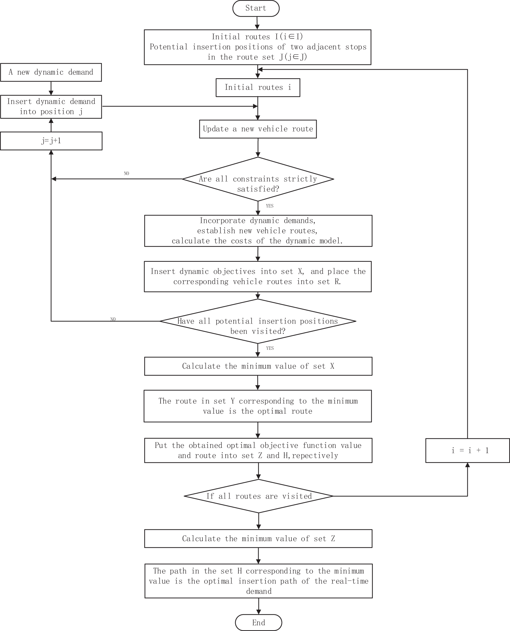
Figure 4: Flowchart of the optimal insertion algorithm

4  Case Analysis

4.1 Case in the First Stage

In a district of Shanghai, the road network includes four bus stops (labeled a, b, c, d). Before the demand-responsive bus departs, numerous bus requests are received. After checking, six boarding stops (numbered 1–6) and six alighting stops (numbered 7–12) are established. The placement of these stops within the roadway system is illustrated in Fig. 5. In Fig. 5: White sectors represent bus stops. Orange ovals represent boarding stops. Yellow rounded rectangles represent alighting stops. The connections between nodes indicate connectivity without any other implication. Given the extensive number of stops, it is assumed that all nodes are interconnected within the road network, even if direct links are absent. Table 2 details the passenger count at each boarding stop and the distances to parking lots and alighting stops. Network distance has been used, considering the actual road network and traffic conditions.

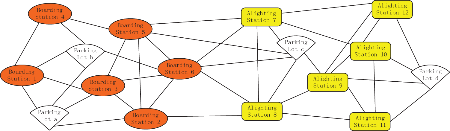
Figure 5: First stage road network diagram

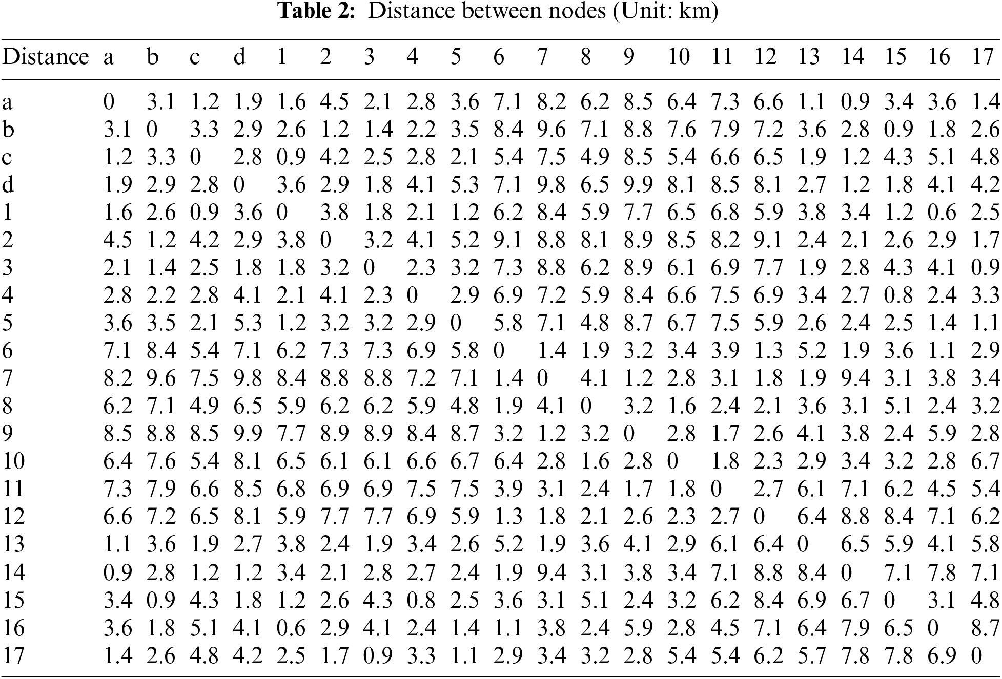
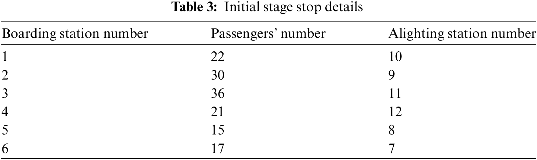
Table 3 provides information about each stop. From Table 3, we can see: Passengers at boarding stop 1 go to alighting stop 10. Passengers at boarding stop 2 go to alighting stop 9. Passengers at boarding stop 3 go to alighting stop 11. Passengers at boarding stop 4 go to alighting stop 12. Passengers at boarding stop 5 go to alighting stop 8. Passengers at boarding stop 6 go to alighting stop 7.

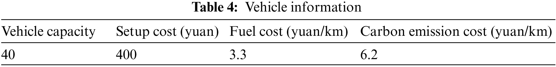
The study’s key parameters include: Vehicle capacity: 40 persons/vehicle. Average travel speed: 40 km/h. Unit transportation cost with passengers: 200 yuan/km. Empty load cost: 50 yuan/km. Fixed vehicle cost: 400 yuan/vehicle. Average boarding time per passenger: 3 s. Fuel cost for a 40-seat vehicle: 3.3 yuan/km [37]. Maximum operation time: 720 min. Passenger travel time window: 5 min. Number of potential stops: 17. A route optimization plan must be created before the bus departs to minimize both operational costs and passenger travel time.

Table 4 displays the parameter settings for the initial vehicle route optimization model.

In the first stage, the route is optimized based on the initial travel demands received by the roadway system before the leaving of the demand-responsive bus. The proposed solution algorithm is implemented in Java, using a population size of 200, running for a maximum of 200 generations, with crossover probability set to 0.8 and mutation probability set to 0.1. After a runtime of 29.6 s, it successfully optimized the initial stage of demand-responsive bus routes, yielding the Pareto solution set. Detailed outcomes are presented in Tables 5 and 6.

Fig. 6 displays these solutions. Both Pareto solutions in Fig. 6 effectively minimize passenger travel time and operational costs.

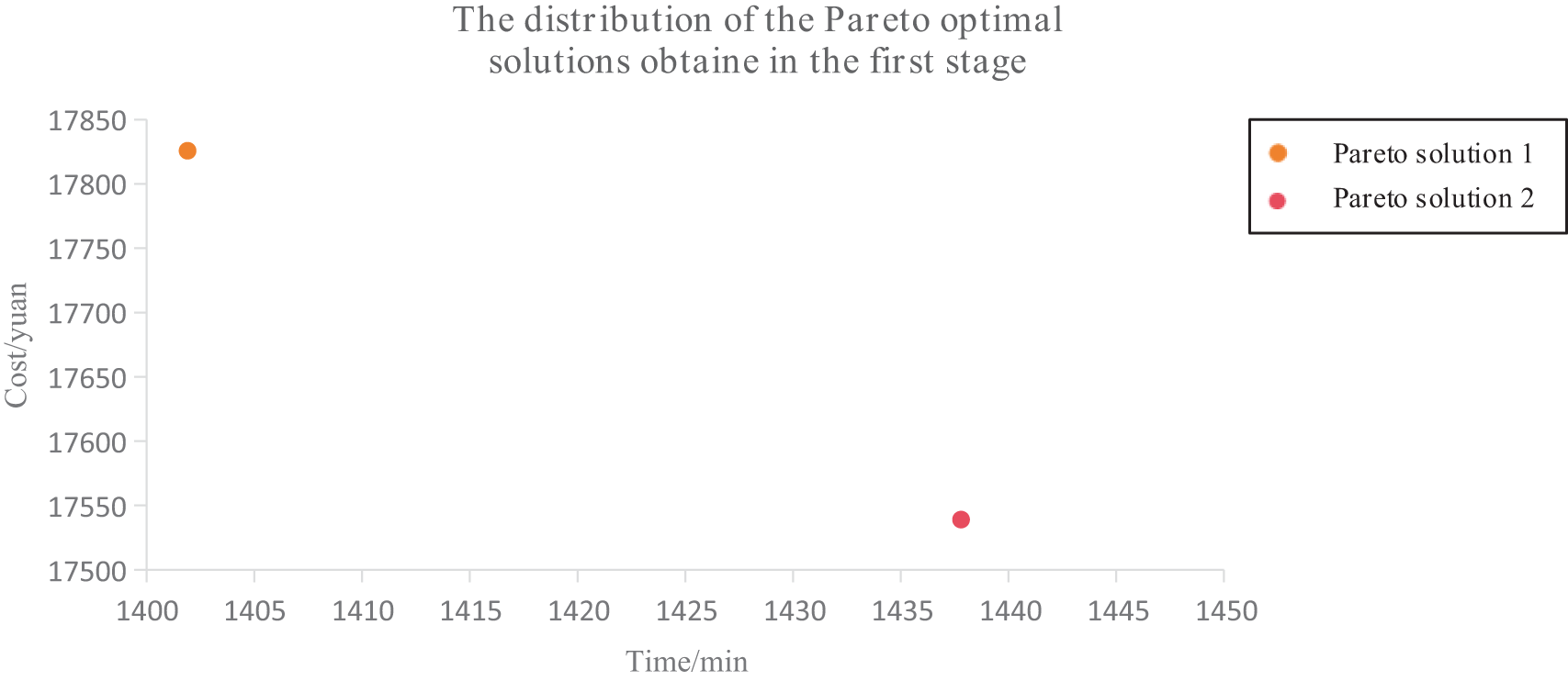
Figure 6: The allocation of the two Pareto-optimal solutions achieved in the first stage

(1) Result Comparison 1: The time of passengers’ journey. According to Tables 5 and 6, there is the whole travel time of 1401.9 min in Pareto Solution 1. It sends two buses from parking lot a to serve boarding stops 1, 6, and 3, transporting passengers to alighting stops 7, 10, and 11, and then stopping at parking lots c and d, taking 629.6 min. Parking lot b sends two buses to serve boarding stops 4, 5, and 2, transporting passengers to alighting stops 8, 12, and 9, taking 598.8 min. There is the whole travel time of 1401.9 min in Pareto Solution 2. It sends two buses from parking lot a to serve boarding stops 1, 5, and 2, transporting passengers to alighting stops 10, 8, and 9, taking 629.6 min. It sends two buses from parking lot b. The first bus picks up 36 passengers, transports them to the alighting stop, and returns to parking lot c; the second bus follows route b-3-11-d, serving boarding stop 3 and alighting stop 11, taking 363.6 min.

(2) Result Comparison 2: Tables 5 and 6 show the operational cost for two buses is 8880.86 yuan from parking lot a in Pareto Solution 1. For parking lot b, the cost is 8944.9 yuan, including vehicle costs, making the total 17,825.76 yuan. It sends two buses for three boarding stops from parking lot a in Pareto Solution 2, then three alighting stops, finally returning to parking lot c and d, costing 9212.96 yuan. Parking lot b sends two buses for three boarding stops and three alighting stops, costing 8326.3 yuan, plus a fixed vehicle cost of 400 yuan, totaling 17,539.26 yuan.

Fig. 7 shows Total passenger travel time for Pareto Solutions 1 and 2. There is the whole travel time of 1401.9 min in Pareto Solution 1, while Pareto Solution 2 has 1437.8 min. This means Pareto Solution 1 reduces travel time by 35.9 min. From a passenger perspective, shorter travel time is preferable, making Pareto Solution 1 more attractive.

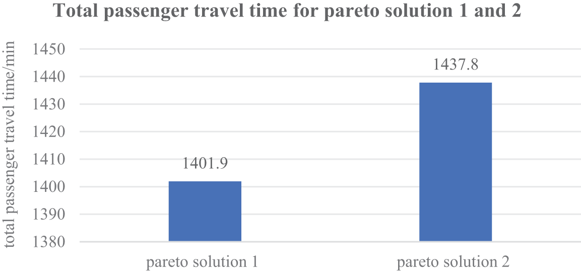
Figure 7: Total passenger travel time for Pareto Solutions 1 and 2

Fig. 8 compares the total operational costs for the demand-responsive bus company under both Pareto solutions. Pareto Solution 1 incurs 286.47 yuan more in operational costs than Pareto Solution 2. Thus, adopting Pareto Solution 2 can save costs for the bus company.

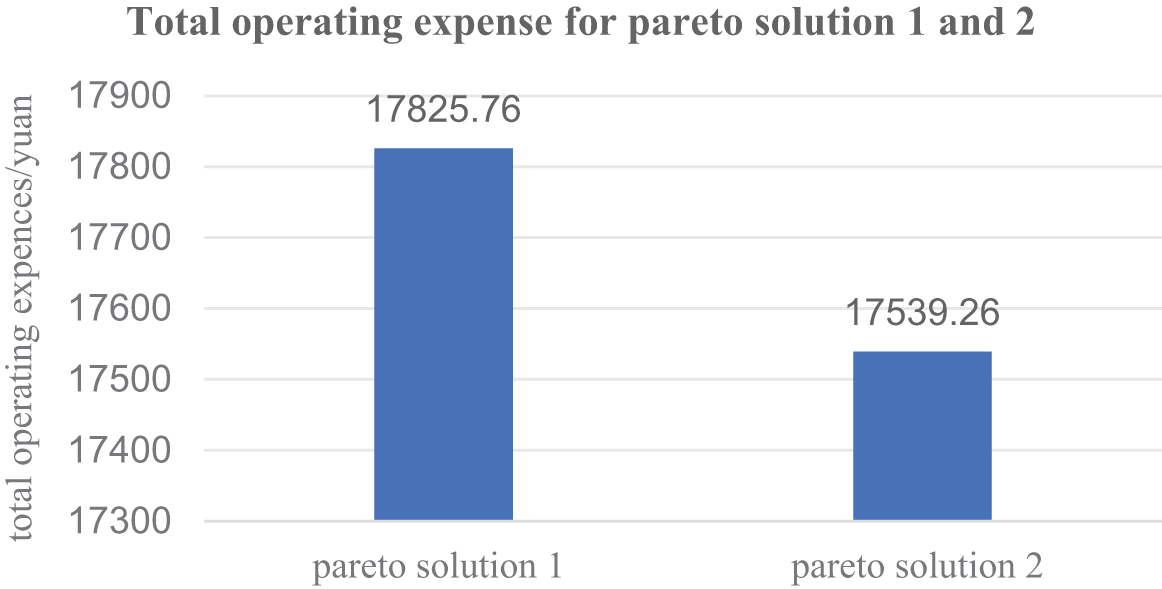
Figure 8: Total operating expense for Pareto Solutions 1 and 2

In summary, Figs. 7 and 8 demonstrate that two Pareto Solutions have distinct superiority in reducing total passenger travel time and operational costs for the bus company. Pareto Solution 1 reduces passenger travel time by 35.9 min compared to Pareto Solution 2, making it more beneficial for passengers. From the bus company’s perspective, Pareto Solution 2 saves 286.47 yuan in operational costs compared to Pareto Solution 1, making it more cost-effective. However, the final route optimization scheme should be chosen with comprehensive consideration to avoid disadvantaging either party.

Tables 7 and 8 demonstrate that expanding the time window allows vehicles to serve more passengers, significantly increasing the response rate. To meet real-time demands, vehicles may need to make detours, pass stops, and alter routes, inevitably increasing the average time passengers spend on the bus and time. The results confirm that as the time window expands, both the total operational cost for vehicles and the average time passengers spend on the bus increase. When the time window is shorter, passenger waiting time can be somewhat reduced, but the number of rejected passengers increases rapidly, adversely affecting the attractiveness of public transportation. Although a longer time window allows more passengers to be served, the waiting time and time spent on the bus increase sharply, reducing passengers’ willingness to travel. When the time window is at an intermediate level, operational travel costs and penalty costs decrease, particularly when the time window is set to 15 min. Therefore, to achieve better results, this study will set the time window to 15 min in subsequent experiments.

4.2 Case in the Second Stage

In the first stage, initial passenger requests before departure were screened and processed to form 6 boarding stops and 6 corresponding alighting stops. The improved NSGA-II algorithm solved the model, yielding two Pareto solutions. The second stage involves immediate route improvement based on the results from the first stage.

Because the demand-responsive bus should update its route in real time whenever there are real-time requests within the response range before leaving the boarding area, the number of responses will vary based on the number of real-time requests. Each response requires recalculating the model. The second stage proposes generating real-time travel requests at 3-min intervals. Assuming that at the 3-min mark, based on real-time travel requests generated in the roadway system, the bus corporation processes and adds 3 new boarding stops (numbered 13–15) and 3 new alighting stops (numbered 16–18). The road network for the second stage is shown in Fig. 9. In Fig. 9, the orange nodes indicate stops serviced by the demand-responsive bus within 3 min. This frequency is chosen based on a balance between responsiveness to real-time passenger demands and computational efficiency. Generating requests too frequently (e.g., every minute) could lead to excessive computational overhead, making the optimization process too slow to be practical for real-time applications. On the other hand, generating requests too infrequently (e.g., every 10 min) might result in delayed responses to passenger needs, reducing the effectiveness of the demand-responsive system. The 3-min interval ensures timely responses to passenger requests and manageable computational loads, allowing near real-time updates to routes and schedules, thereby enhancing service quality and passenger satisfaction. Parallelograms and diamonds represent the newly formed boarding and alighting stops based on real-time passenger requests at the 3-min mark. Relevant information for each stop is provided in Table 9. According to Table 9: Passengers at boarding stop 13 need to go to alighting stop 17. Passengers at boarding stop 14 need to go to alighting stop 16. Passengers at boarding stop 15 need to go to alighting stop 18. Table 2 provides the distances between nodes. All parameters remain consistent with the first stage. The second stage aims to minimize total operational costs and passenger travel time through real-time route optimization of demand-responsive bus routes.

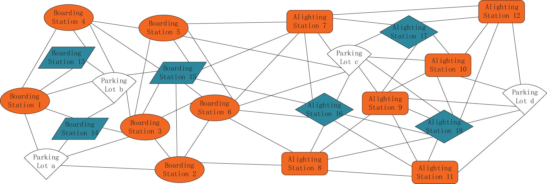
Figure 9: Second stage road network diagram

The proposed solution algorithm, implemented in Java, is used in this stage. The optimized route for the second stage was obtained after running for 36.7 s. Detailed results are presented in Tables 10 and 11. Comparing the second stage scheme with the first stage shows differences due to increased boarding and alighting stops and the available seat count on buses for new real-time requests. Additionally, the initial position of every bus upon receiving real-time requests must be determined to improve the route.

Tables 10 and 11 show the real-time stage optimization scheme. Fig. 10 illustrates the arrangement of these results.

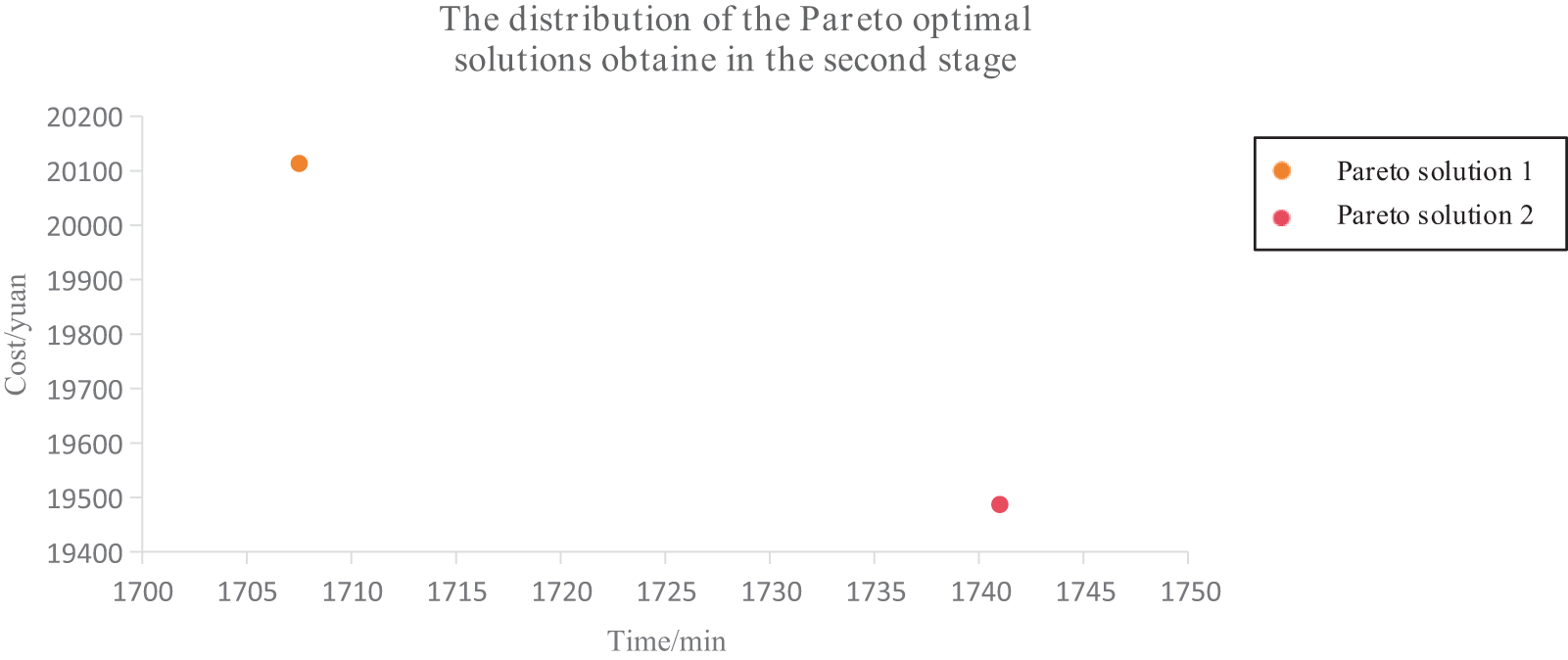
Figure 10: The allocation of the two Pareto-optimal solutions achieved in the first stage

(1) Result Comparison 1: The time of passengers’ journey. Tables 10 and 11 show that Pareto Solution 1 uses 4 demand-responsive buses. It sends two buses in parking lot a. The first bus follows the route a-1-6-10-7-c departing from parking lot a, stopping at boarding stops 1 and 6 to pick up passengers. After stop 6, the bus has 39 passengers. With this number, it cannot pick up more passengers at the next stop. It then proceeds to alighting stops 10 and 7, and returns to parking lot c, taking 471.9 min in total. The second bus follows route a-3-13-11-17-d, carrying 39 passengers. It serves two boarding and two alighting stops, taking 405.6 min. Parking lot b also sends two buses. The first bus follows route b-4-5-15-12-8-18-c. After picking up passengers at stops 4, 5, and 15, the bus is full with 40 passengers. It then proceeds to the alighting stops, completing the route in 508 min. The second bus follows route b-2-14-9-16-d, carrying 35 passengers and taking 322 min. Pareto Solution 2 uses 4 demand-responsive buses, with dispatching two buses from parking lots. The first bus follows route a-1-5-13-10-8-17-c departing from parking lot a, stopping at boarding stops 1, 5, and 13. After these stops, the bus is full. It then proceeds to alighting stops 10, 8, and 17, and returns to parking lot c, taking 436 min in total. The second bus follows route a-2-14-16-9-d, carrying 35 passengers and taking 388.5 min. It sends two buses for the remaining passengers from parking lot b. The first bus follows route b-4-6-12-7-c, carrying 38 passengers and taking 444.6 min. The second bus follows route b-3-13-17-11-d, carrying 39 passengers and taking 471.9 min.

Fig. 11 compares the total passenger travel time for Pareto Solutions 1 and 2 in the second stage. As depicted in Fig. 11, Pareto Solution 1 has a total travel time of 1707.5 min, whereas Pareto Solution 2 has 1741 min. Thus, Pareto Solution 2’s travel time is 33.5 min longer than that of Pareto Solution 1. These results suggest that Pareto Solution 1 is better for minimizing total passenger travel time, allowing passengers to complete their trips more quickly.

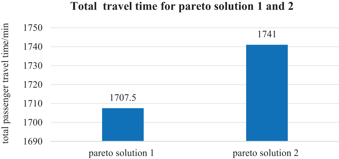
Figure 11: Total travel time for Pareto Solutions 1 and 2

(2) Result Comparison 2: Total Operational Expense for the Demand-Responsive Bus Firm. Fig. 12 compares the total operational costs for the bus company between Pareto Solutions 1 and 2 in the second stage. As shown, there is a total cost of 20,113.4 yuan in pareto solution 1, whereas Pareto Solution 2 costs 19,487.02 yuan. The costs for Pareto Solution 1 include 9867.96 yuan from parking lot a and 10,245.44 yuan from parking lot b. For Pareto Solution 2, the costs are 10,101.76 yuan for parking lot a and 9385.26 yuan for parking lot b. Fig. 12 indicates that Pareto Solution 2 saves 626.38 yuan, making it more cost-effective than Pareto Solution 1. Minimizing operational costs while meeting passenger demands is crucial for the bus company. Therefore, the company would likely choose Pareto Solution 2.

Figure 12: Total operating expense for Pareto Solutions 1 and 2

In conclusion, Figs. 11 and 12 show that Pareto Solutions 1 and 2 each have benefits in minimizing passenger travel time and operational costs, respectively. Pareto Solution 1 is 33.5 min shorter in travel time, increasing passenger satisfaction. Conversely, Pareto Solution 2 is 626.38 yuan cheaper, making it more attractive for the bus company. Passengers and the bus company have conflicting interests. Solely pursuing one party’s interests harms the other. Thus, a balanced route optimization plan that considers both parties’ interests is necessary.

4.3 Case Analysis

The two-stage route optimization results are analyzed as follows.

Since the second stage builds on the first, it is assumed that real-time travel requests do not exceed the total capacity of the buses used in the first stage. The second stage uses the same number of remaining seats and vehicles as the first, requiring 4 buses to meet the demand of 183 passengers. Similarly, the first bus route in Pareto Solution 2 is the same in both stages: b-4-6-12-7-c. This indicates that some first-stage optimized routes cannot accommodate real-time requests in the second stage. This may be due to two reasons: First, if first-stage vehicles have a high occupancy rate, remaining seat capacity may not accommodate new passengers. Second, real-time request locations may be outside the service range or far from the travel routes of certain vehicles. These findings highlight the need to consider real-time requests in real-time and adjust routes to balance operational efficiency and passenger satisfaction.

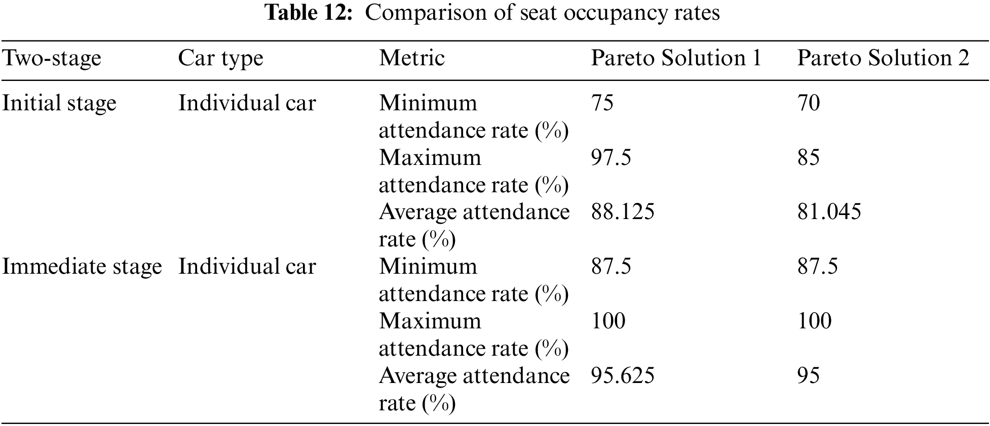
In the second stage, optimized bus routes achieved higher occupancy rates than in the first stage. This improvement is seen in both individual and average occupancy rates. Details are provided in Table 12. There are minimum, maximum, and average occupancy rates of 75.0%, 97.5%, and 88.125% in Pareto Solution 1 in the first stage, respectively. For Pareto Solution 2, these rates were 70%, 85%, and 81.045%, respectively. The average occupancy rate for the initial phase was 84.585%. There are minimum, maximum, and average rates of 87.5%, 100.0%, and 95.625% in the second stage in Pareto Solution 1, respectively. For Pareto Solution 2, these rates were 87.5%, 100.0%, and 95%. The average seat utilization for the immediate phase was 95.3125%. In comparison to the initial phase, the average occupancy increased by 10.7275%, with individual buses improving by up to 17.5%. Except for 2 buses on the same routes, the two-stage method resulted in a significant improvement in occupancy rates. Without the two-stage method, two issues might arise. First, if real-time requests aren’t timely serviced, more empty seats waste resources. Second, dispatching a new bus for real-time requests increases operational costs. Thus, the two-stage method effectively addresses immediate requests, optimizing occupancy and minimizing costs.

To validate the improved NSGA-II genetic algorithm, it was compared to the traditional NSGA-II algorithm in solving the vehicle scheduling problem under the muti-objective DRT service model. Both algorithms used the same parameters: population size of 100, crossover probability of 0.8, mutation probability of 0.1, and 100 iterations. Fig. 13 shows the results of the two algorithms. As shown, the improved NSGA-II algorithm has significant advantages in convergence speed and objective function results. According to Table 13, compared to the traditional NSGA-II algorithm, although average in-vehicle time for passengers increased by 1.9%, the number of trips and total travel time decreased by 25.9% and 13.1%, respectively, effectively improving vehicle utilization. The runtime of the improved NSGA-II algorithm was reduced by 4.8%, demonstrating its effectiveness.

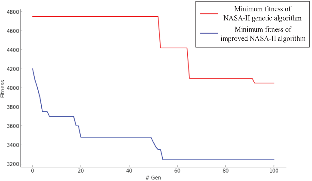
Figure 13: Comparison of results of improved genetic algorithm and traditional algorithm

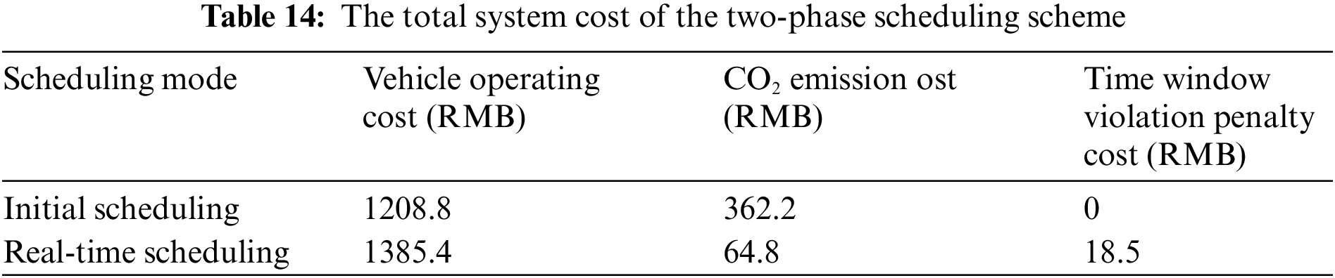
Unlike the initial scheduling stage, where initial routes are generated based on subscription demands, the real-time scheduling stage involves vehicles receiving real-time requests during operation. The vehicle routes are dynamically adjusted according to time windows, boarding, and alighting points. The adjusted routes will change passengers’ in-vehicle time, the number of served passengers, vehicle operation time, and other factors. The following experiment aims to observe the changes in travel expense and passengers’ number who has been served when applying the real-time scheduling stage during operation. The specific results are shown in Tables 13 and 14.

5  Conclusion

This paper explores real-time demand-responsive bus route optimization using a two-stage way to handle immediate travel requests and achieve route updates. A multi-objective optimization model is developed, aiming to minimize vehicle operation costs, travel costs, CO2 emissions, time window deviations, and penalties for rejecting passengers, taking into account the interests of both passengers and operators. An improved NSGA-II genetic algorithm is proposed to address immediate bus route improvement with random user demands. The first stage addresses initial travel requests, generating an initial optimized bus route. The second stage manages real-time travel requests, updating the bus route accordingly. An insertion algorithm is designed to handle the model’s characteristics.

To verify the model and method’s effectiveness, they were applied to a two-stage case study for comparison. Analysis results show: (1) Using existing vehicles for real-time travel requests, instead of dispatching new ones from the parking lot, can save operational costs. (2) With the same demand, setting the time window too large can rapidly increase waiting time, while setting it too small can drastically reduce the number of served passengers. (3) Using real-time scheduling increases vehicle operating costs by 12.6% and reduces CO2 emission costs by 82.1%. This serves more passengers, greatly improves vehicle utilization, and significantly reduces CO2 emission costs. Despite slightly higher operational and detour costs, the method attracts more passengers by reducing penalties for rejecting passengers and deviating from passenger time windows.

This study assumes vehicle speed to be constant, without considering the impact of real-time factors on speed, simplified assumptions and limited real-time data usage. Additionally, the consideration of multiple stops is limited. Future research can focus on various potential improvements, such as the cost and comfort of different vehicle types, the impact of real-time road condition changes on vehicle speed, modeling passenger comfort, integration with intelligent transportation systems, and advanced data analysis. These efforts aim to ultimately enhance urban mobility and passenger experience.

Acknowledgement: The authors would like to express their heartfelt gratitude to the editors and reviewers for their detailed review and insightful advice.

Funding Statement: The authors received no specific funding for this study.

Author Contributions: The authors confirm contribution to the paper as follows: Study conception and design: Jingfa Ma, Hu Liu and Lingxiao Chen; data collection: Lingxiao Chen; analysis and interpretation of results: Jingfa Ma; draft manuscript preparation: Jingfa Ma. All authors reviewed the results and approved the final version of the manuscript.

Availability of Data and Materials: The data and codes that support the findings of this study are available from the corresponding authors upon reasonable request.

Ethics Approval: Not applicable.

Conflicts of Interest: The authors declare that they have no conflicts of interest to report regarding the present study.

References

1. J. Qin, Y. Lin, T. Wu, X. Lin, and X. Li, “A spatio-temporal perspective on commercial vehicle travel patterns in urban environments,” IEEE Access, vol. 12, pp. 91447–91461, 2024. doi: 10.1109/ACCESS.2024.3421554. [Google Scholar] [CrossRef]

2. M. Yu, T. Yang, C. Li, Y. Jin, and Y. Xu, “Mitigating bus bunching via hierarchical multi-agent reinforcement learning,” IEEE Trans. Intell. Transp. Syst., vol. 25, no. 8, pp. 9675–9692, Aug. 2024. doi: 10.1109/TITS.2024.3362813. [Google Scholar] [CrossRef]

3. B. A. Kumar, G. H. Prasath, and L. Vanajakshi, “Dynamic bus scheduling based on real-time demand and travel time,” Int. J. Civil Eng., vol. 17, no. 9, pp. 1481–1489, 2019. doi: 10.1007/s40999-019-00445-y. [Google Scholar] [CrossRef]

4. Y. H. Kuo, M. Y. Leung, and Y. Yan, “Public transport for smart cities: Recent innovations and future challenges,” Eur. J. Oper. Res., vol. 306, no. 3, pp. 1001–1026, May 2023. doi: 10.1016/j.ejor.2022.06.057. [Google Scholar] [CrossRef]

5. T. Liu and A. A., “Ceder analysis of a new public-transport-service concept: Customized bus in China,” Transp. Policy, vol. 39, no. 4, pp. 63–76, Apr. 2015. doi: 10.1016/j.tranpol.2015.02.004. [Google Scholar] [CrossRef]

6. R. Curtale, F. Liao, and P. Waerden, “Understanding travel preferences for user-based relocation strategies of one-way electric car-sharing services,” Transp. Res. Part C: Emerg. Technol., vol. 127, no. 3, Jun. 2021, Art. no. 103135. doi: 10.1016/j.trc.2021.103135. [Google Scholar] [CrossRef]

7. K. Liu, J. Liu, and J. Zhang, “Heuristic approach for the multiobjective optimization of the customized bus scheduling problem,” IET Intel. Transp.Syst, vol. 16, no. 3, pp. 277–291, Dec. 2021. doi: 10.1049/itr2.12131. [Google Scholar] [CrossRef]

8. Y. Cheng, A. Huang, G. Qi, and B. Zhang, “Mining customized bus demand spots based on smart card data: A case study of the beijing public transit system,” IEEE Access, vol. 7, pp. 181626–181647, 2019. doi: 10.1109/ACCESS.2019.2959907. [Google Scholar] [CrossRef]

9. J. Hansson, F. Pettersson-Löfstedt, H. Svensson, and A. Wretstrand, “Patronage effects of off-peak service improvements in regional public transport,” Eur. Transp. Res. Rev., vol. 14, no. 1, May 2022, Art. no. 19. doi: 10.1186/s12544-022-00543-4. [Google Scholar] [CrossRef]

10. A. S. A. Maria, R. M. Soe, and M. A. Saif, “Framework for connecting the mobility challenges in low density areas to smart mobility solutions: The case study of Estonian municipalities,” Eur. Transp. Res. Rev., vol. 14, no. 1, pp. 32, Jul. 2022. doi: 10.1186/s12544-022-00557-y. [Google Scholar] [CrossRef]

11. J. Zhao, S. Sun, and O. Cats, “Joint optimisation of regular and demand-responsive transit services,” Transp. A: Transp. Sci., vol. 19, no. 2, Feb. 2023, Art. no. 1987580. doi: 10.1080/23249935.2021.1987580. [Google Scholar] [CrossRef]

12. Z. Wang, J. Yu, W. Hao, and J. Xiang, “Joint optimization of running route and scheduling for the mixed demand responsive feeder transit with time-dependent travel times,” IEEE Trans. Intell. Transp. Syst., vol. 22, no. 4, pp. 2498–2509, Apr. 2021. doi: 10.1109/TITS.2020.3041743. [Google Scholar] [CrossRef]

13. X. B. Zhan, W. Y. Szeto, C. S. Shui, and X. Q. Chen, “A modified artificial bee colony algorithm for the dynamic ride-hailing sharing problem,” Transp. Res. Part E: Logist. Transp. Review, vol. 150, no. 9, Jun. 2021, Art. no. 102124. doi: 10.1016/j.tre.2020.102124. [Google Scholar] [CrossRef]

14. H. Wang, H. Guan, H. Qin, W. Li, and J. Zhu, “A slack departure strategy for demand responsive transit based on bounded rationality,” J. Adv. Transp., vol. 2022, pp. 1–16, May 2022. doi: 10.1155/2022/9693949. [Google Scholar] [CrossRef]

15. C. Wang, C. Ma, and X. Xu, “Multi-objective optimization of real-time customized bus routes based on two-stage method,” Phys. A, Stat. Mech. Appl., vol. 537, no. 8, Jan. 2020, Art. no. 122774. doi: 10.1016/j.physa.2019.122774. [Google Scholar] [CrossRef]

16. C. Shen, Y. Sun, Z. Bai, and H. Cui, “Real-time customized bus routes design with optimal passenger and vehicle matching based on column generation algorithm,” Phys. A, Stat. Mech. Appl., vol. 571, no. 1, Jun. 2021, Art. no. 125836. doi: 10.1016/j.physa.2021.125836. [Google Scholar] [CrossRef]

17. X. Chen, Y. Wang, Y. Wang, X. Qu, and X. Ma, “Customized bus route design with pickup and delivery and time windows: Model, case study and comparative analysis,” Exp. Syst. Appl., vol. 168, no. 6, Apr. 2021, Art. no. 114242. doi: 10.1016/j.eswa.2020.114242. [Google Scholar] [CrossRef]

18. L. Sörensen, A. Bossert, J. Jokinen, and J. Schlüter, “How much flexibility does rural public transport need? –Implications from a fully flexible DRT system,” Transp. Policy, vol. 100, no. 8, pp. 5–20, Jan. 2021. doi: 10.1016/j.tranpol.2020.09.005. [Google Scholar] [CrossRef]

19. J. Berrada and A. Poulhès, “Economic and socioeconomic assessment of replacing conventional public transit with demand responsive transit services in low-to-medium density areas,” Transp. Res. Part A: Policy. Pract., vol. 150, no. 9, pp. 317–334, Aug. 2021. doi: 10.1016/j.tra.2021.06.008. [Google Scholar] [CrossRef]

20. L. He, J. Li, and J. Sun, “How to promote sustainable travel behavior in the post COVID-19 period: A perspective from customized bus services,” Int. J. Transp. Sci. Technol., vol. 12, no. 1, pp. 19–33, Mar. 2023. doi: 10.1016/j.ijtst.2021.11.001. [Google Scholar] [CrossRef]

21. Y. Gu and A. Chen, “Modeling mode choice of customized bus services with loyalty subscription schemes in multi-modal transportation networks,” Transp. Res. Part C: Emerg. Technol., vol. 147, no. 4, p. 104012, Feb. 2023. doi: 10.1016/j.trc.2023.104012. [Google Scholar] [CrossRef]

22. W. Ma, Y. Guo, K. An, and L. Wang, “Pricing method of the flexible bus service based on cumulative prospect theory,” J. Adv. Transport., vol. 2022, no. 1, Mar. 2022. doi: 10.1155/2022/1785199. [Google Scholar] [CrossRef]

23. J. Li, X. Feng, and B. Jia, “Pricing game between customized bus and conventional bus with combined operational objectives,” Systems, vol. 10, no. 3, Apr. 2022, Art. no. 55. doi: 10.3390/systems10030055. [Google Scholar] [CrossRef]

24. J. Zhang, G. Ren, and J. Song, “Resilience-based optimization model for emergency bus bridging and dispatching in response to metro operational disruptions,” PLoS One, vol. 18, no. 3, Mar. 2023, Art. no. e0277577. doi: 10.1371/journal.pone.0277577. [Google Scholar] [PubMed] [CrossRef]

25. F. Altarifi, N. Louzi, D. Abudayyeh, and T. Alkhrissat, “User preference analysis for an integrated system of bus rapid transit and on-demand shared mobility services in amman, jordan,” Urban Sci., vol. 7, no. 4, Oct. 2023, Art. no. 111. doi: 10.3390/urbansci7040111. [Google Scholar] [CrossRef]

26. S. Mishra and B. Mehran, “Optimal design of integrated semi-flexible transit services in low-demand conditions,” in IEEE Access, Mar. 2023, vol. 11, pp. 30591–30608, doi: 10.1109/ACCESS.2023.3260727. [Google Scholar] [CrossRef]

27. Z. Xie, R. Qiu, S. Wang, X. Tan, Y. Xie, and L. Ma, “PIG: Prompt images guidance for night-time scene parsing,” IEEE Trans. Image Process., vol. 33, pp. 3921–3934, 2024. doi: 10.1109/TIP.2024.3415963. [Google Scholar] [PubMed] [CrossRef]

28. D. Xia, L. Zheng, X. Cai, W. Liu, and D. Sun, “Urban customized bus design for private car commuters,” IEEE Inter. Things J., vol. 9, no. 21, pp. 21723–21735, Nov. 2022. doi: 10.1109/JIOT.2022.3181591. [Google Scholar] [CrossRef]

29. V. Katerina, K. Katerina, A. Ivetta, and G. Andrii, “Designing optimal public bus route networks in a suburban area,” Transp. Res. Procedia, vol. 39, no. 2, pp. 554–564, 2019. doi: 10.1016/j.trpro.2019.06.057. [Google Scholar] [CrossRef]

30. D. Guan, X. Wu, K. Wang, and J. Zhao, “Vehicle dispatch and route optimization algorithm for demand-responsive transit,” Processes, vol. 10, no. 12, Dec. 2022, Art. no. 2651. doi: 10.3390/pr10122651. [Google Scholar] [CrossRef]

31. S. Kale and P. Das Gupta, “Planning for demand responsive bus service for limited area using simulation,” in Lecture Notes in Civil Engineering, D. Singh, L. Vanajakshi, A. Verma, and A. Das, Eds., Singapore: Springer, 2022, vol. 218. doi: 10.1007/978-981-16-9921-4_2. [Google Scholar] [CrossRef]

32. X. Zhou, G. Wei, Y. Zhang, Q. Wang, and H. Guo, “Optimizing multi-vehicle demand-responsive bus dispatching: A rea-time reservation-based approach,” Sustainability, vol. 15, no. 7, Mar. 2023, Art. no. 5909. doi: 10.3390/su15075909. [Google Scholar] [CrossRef]

33. B. Zhang, Z. Zhong, X. Zhou, Y. Qu, and F. Li, “Optimization model and solution algorithm for rural customized bus route operation under multiple constraints,” Sustainability, vol. 15, no. 5, Feb. 2023, Art. no. 3883. doi: 10.3390/su15053883. [Google Scholar] [CrossRef]

34. X. Li, T. Wang, W. Xu, H. Li, and Y. Yuan, “A novel model and algorithm for designing an eco-oriented demand responsive transit (DRT) system,” Transp. Res. Part E: Logist. Transp. Review, vol. 157, no. 3, Jan. 2022, Art. no. 102556. doi: 10.1016/j.tre.2021.102556. [Google Scholar] [CrossRef]

35. L. Wang, L. Zeng, W. Ma, and Y. Guo, “Integrating passenger incentives to optimize routing for demand-responsive customized bus systems,” IEEE Access, vol. 9, pp. 21507–21521, Feb. 2021. doi: 10.1109/ACCESS.2021.3055855. [Google Scholar] [CrossRef]

36. M. B. D. Galarza, K. Sörensen, and P. Vansteenwegen, “A large neighborhood search algorithm to optimize a demand-responsive feeder service,” Transp. Res. Part C: Emerg. Technol., vol. 127, no. 2, Jun. 2021, Art. no. 103102. doi: 10.1016/j.trc.2021.103102. [Google Scholar] [CrossRef]

37. M. Sedong, K. Seung-Young, K. Dong-Kyu, and C. Shin-Hyung, “Performance measurement and determination of introduction criteria for peak demand responsive transit service,” J. Korean Soc. Transp., vol. 39, no. 1, pp. 100–114, Feb. 2021. doi: 10.7470/jkst.2021.39.1.100. [Google Scholar] [CrossRef]

38. Y. Hou, T. Liu, H. Hu, and B. Du, “Optimal routing design of demand-responsive feeder transit in the era of mobility as a service,” in 2022 IEEE 25th Int. Conf. Intell. Transp. Syst. (ITSC), Macau, China, 2022, pp. 3405–3410. doi: 10.1109/ITSC55140.2022.9922343. [Google Scholar] [CrossRef]

39. D. X. Wu and X. B. Duan, “Analysis of time characteristics of buses on and off in Huai’an city,” Logist Eng. Manage., vol. 39, no. 12, pp. 109–114, Dec. 2017. [Google Scholar]