Continual Reinforcement Learning for Intelligent Agricultural Management under Climate Changes

1  Introduction

As climate change exacerbates, farmers find it increasingly challenging to conduct various field operations necessary to meet specific production targets during growing seasons affected by extreme weather conditions like heatwaves and droughts. Simultaneously, according to data from the Food and Agriculture Organization (FAO), approximately 828 million people still faced hunger in 2022. In light of this urgent issue, adopting new technologies to enhance agricultural output is crucial. One such technology is Precision Agriculture (PA) [1]. Precision agriculture, also known as “precision farming” or “prescription farming,” is an increasingly significant field focused on enhancing the efficiency and sustainability of agricultural practices. This discipline leverages cutting-edge technologies such as remote sensing, robotics, Machine Learning (ML), and Artificial Intelligence (AI) to improve crop management. Precision agriculture involves monitoring plant health parameters like water levels, temperature, etc. It enables farmers to accurately determine the necessary conditions for optimal crop health, including the specific needs for water and nutrients and the precise timing and location for their application. This approach requires collecting extensive data from various sources across different parts of the field, such as soil nutrients, pest and weed presence, chlorophyll content in plants, and certain weather conditions. In today’s increasingly complex climate scenarios, reinforcement learning (RL) [2] can effectively address such challenges, enabling an agent to maximize the expected return through a well-designed model in a dynamic and variable environment.

As one subset of ML, RL empowers computer programs, acting as agents, to control unknown and uncertain dynamical systems while pursuing specific tasks [3,4]. This approach has garnered increasing attention from researchers interested in determining optimal strategies for agricultural management. Gautron et al. [5] extended the DSSAT [6], a widely recognized agricultural simulation tool that can model crop outcomes under different environmental scenarios, to a realistic simulation environment known as Gym-DSSAT. In this simulation environment, RL agents can learn effective fertilization and irrigation strategies by utilizing soil properties and historical or forecasted weather data. Wu et al. [7] have shown that RL-trained policies can surpass traditional methods, achieving comparable or higher crop yields with less fertilizer use, marking a significant step toward sustainable agriculture. Additionally, Sun et al. [8] have demonstrated the potential of RL in irrigation control by optimizing water usage without compromising crop health, further highlighting Gym-DSSAT’s capability in efficient resource management. Moreover, Wang et al. [9] have confirmed the robustness of learning-based fertilization management, even under difficult conditions. Despite extreme weather scenarios, the RL agents proved capable of learning optimal policies, leading to very satisfactory outcomes. They also improved the quantification of uncertainty in the performance of these optimal policies. The agents could develop adaptive fertilization and irrigation strategies, particularly in response to climate changes such as increasing temperatures and decreasing rainfall [10].

Many existing studies have primarily considered agricultural environments to be fully observable and, as a result, have framed the corresponding RL challenges within the context of Markov Decision Processes (MDPs). Within MDPs, it is presumed that each environmental state provides all the essential information an agent needs to select the best action to meet the objective function. Nonetheless, this approach encounters considerable difficulties when applied to real-world situations, where agents frequently do not have full knowledge to precisely assess the environment’s state, often due to their observations’ uncertain or incomplete nature. In particular, some state variables in Gym-DSSAT, like the plant water stress index, daily nitrogen denitrification, and daily nitrogen uptake by the plant population, can present difficulties regarding measurement and accessibility. Our previous study [9] explored this issue and found that Partially Observable Markov Decision Processes (POMDPs) can effectively tackle it. We utilized Recurrent Neural Networks (RNNs) to manage the history of observations for decision-making in fertilization management. Our results showed that treating the agricultural environment as a POMDP led to more effective policies than those derived from the traditional assumption of a fully observable MDP [9].

Our prior research [10] also indicated that the pre-learned policies were somewhat adaptable under climate variability. However, they were only effective under minor climate changes, such as temperature variations of around 2 degrees Celsius and precipitation reduction of up to 20%. When faced with more drastic changes, such as significant temperature rises or major decreases in precipitation, these agents would require retraining for new agricultural management strategies to optimize their performance [9]. This limitation underscores the challenges in the model’s generality and adaptability. Simulation results from our earlier studies revealed that the agents’ limited adaptability to extreme weather stemmed from a lack of training under such conditions. We tried to train our model under normal conditions before fine-tuning it under extreme conditions. However, when we applied that model back to normal weather, it resulted in significantly poorer performance. We attribute this issue to catastrophic forgetting, a significant challenge in deep learning today where the agent forgets previously learned information when exposed to new data [11,12]. These challenges motivate our study to seek adaptive policies for agricultural management by employing continual learning (CL), which was proposed by people to overcome catastrophic forgetting and has been actively studied in recent years [13].

Continual learning seeks to emulate the human process and capability of learning. Unlike isolated learning sessions, humans continually integrate and apply past knowledge to new situations [14]. Continual learning embodies this principle through various methodologies, primarily divided into three strategy categories: regularization, distillation, and replay [15]. Regularization restricts updates to the model’s parameters, helping to preserve existing knowledge across different tasks [16]. Examples of regularization techniques include Elastic Weight Consolidation (EWC) [11] and Synaptic Intelligence (SI) [17]. Distillation focuses on transferring knowledge from an older model to a newer one; the older model, which holds previous learning, guides the new model in retaining this information while it learns new content, techniques such as Incremental Moment Matching (IMM) [18] and Learning without Forgetting (LwF) [19] exemplify this strategy. Additionally, replay involves either reusing a subset of original data or generating new samples that mimic the old data’s distribution, aiming to prevent forgetting previously acquired knowledge [20]. Notable replay techniques include Experience Replay (also called Rehearsal) [21] and Gradient Episodic Memory (GEM) [22]. Many researchers have applied CL algorithms to various fields in the past few years and achieved significant success. Maschler et al. [23] applied EWC to help predict the remaining useful life of industrial machinery. They achieved similar performance but reduced the optimization time by a factor of 15 to 30. Shieh et al. [24] applied the experience replay strategy in a one-stage object detection framework for autonomous vehicles and achieved better performance than the state-of-the-art method.

Only a few studies have been reported on various concepts and frameworks of continual reinforcement learning (CRL) methods. Wang et al. [25] introduced a CRL method by merging a policy-based RL method (Deep Deterministic Policy Gradient or DDPG) with the EWC algorithm. Abel et al. [26] did not utilize a specific CL technique in another study. Instead, their agents dynamically updated and refined the policies through ongoing interactions with the environment. In summary, despite the diversity in approaches, all researchers shared the common objective of enhancing the adaptability of RL-induced policies and addressing the issue of catastrophic forgetting in diverse settings.

The main contribution of this study is integrating CL techniques with a DRL method to develop a framework of CRL, which involves continually updating the policy with diverse experiences to adapt to various environments. Our approach is different from transfer learning (TL), which can be applied to RL, and multi-task reinforcement learning (MTRL). Unlike TL that uses knowledge from a previous task to facilitate learning in a new task, our CRL method accumulates knowledge from all previous tasks, allowing it to adapt to a wide range of situations. On the other hand, while MTRL [14] focuses on joint optimization across multiple similar tasks to enable knowledge sharing for improved overall outcomes, it does not accumulate knowledge over time. Our CRL model is designed to optimize a single policy capable of effectively handling various tasks. Furthermore, differing from Wang et al. [25], who employed the EWC technique in a policy-based DRL method, our study tests two CL techniques (EWC and Rehearsal) in a value-based DRL method and evaluates a better combination. Additionally, their CRL method was only applied in fully observable environments [25], while our study marks the first application of CRL methods in the agricultural sector, which involves extreme weather conditions and partially observable environments.

The organization of this paper is as follows: Section 2 introduces the concepts of Partially Observable Markov Decision Processes (POMDPs) and our agricultural simulation environment. It also explores methodologies like Deep Q-learning (DQN) and Proximal Policy Optimization (PPO), discusses continual learning, and outlines the simulation model settings. Additionally, this section defines the specific problems addressed in this paper and develops the CRL framework. Section 3 evaluates and compares various CRL methods, considering normal and extreme weather conditions. This section also considers the impact of climate variability, including higher temperatures and less precipitation, and examines the implications of weather uncertainties. The paper concludes with Section 4, where we summarize our findings, discuss their broader implications, and propose avenues for future research.

2  Methodology

This section starts by introducing the POMPD framework, which was employed to model the agricultural environment and its interaction with intelligent agents in this study. Subsequently, both value-based and policy-based RL approaches and two different CL methods are described. Finally, the problem is defined using the proposed CRL method as the solution approach.

2.1 POMDP and Agriculture Environment

A POMDP is usually represented by P={S,A,T,s0,R,O,Ω},which includes a finite set of states S={s1,…,sn}, a finite set of actions A={a1,…,am}, a finite set of observations O={o1,…,ok}, and the initial state s0∈S. T defines a transition probability T(s,a,s′)=P(st|st−1,at−1). When the agent takes an action a∈A(s) where A(s) is a set of available actions at state s for the agent to take, a transition occurs from the current state s to the next state s′ with a probability T(s,a,s′). Subsequently, the agent receives an observation o∈O with a probability described by Ω(s′,a,o). The main goal of an intelligent agent is to develop an optimal policy that maximizes the expected return, as outlined below. This expected return is the sum of collected rewards beginning from the current state.

U(s)=E∑t=0∞γtR(st,at,st+1)|st=0=s(1)

where st denotes the state of the environment at time t, at is the action to be taken, and R(s,a,s′) is the reward agents can collect after transitioning from state s to s′ by taking action a. It shall be noted that the reward functions are also often written as R(s,a) or R(s). γ∈[0,1] is the discount factor to quantify the importance of rewards collected immediately or in the future.

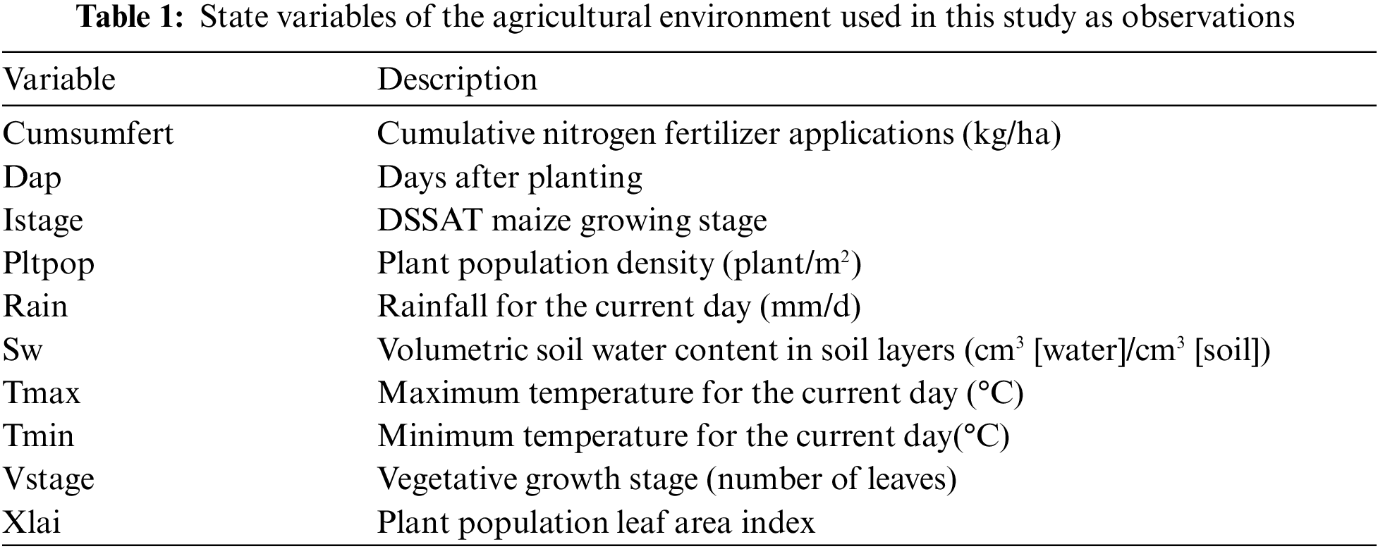
In this study, we utilized Gym-DSSAT [5] as the virtual agricultural environment to simulate crop growth and harvest, as well as nitrate leaching, given weather conditions and the initial soil state. Gym-DSSAT incorporates 28 internal variables representing various environmental states. As noted in our prior work [9], the agricultural environment should be considered partially observable, and ten state variables, as detailed in Table 1, were chosen as the observations. Consequently, agents make decisions based on historical observations, and this approach [9] has been approved to be a more accurate depiction of the decision-making context for the agents, mirroring the complexity encountered in actual agricultural scenarios.

Given that maize crops in Iowa usually rely on rainfall for irrigation [7], this study does not consider daily irrigation but focuses instead on nitrogen fertilization. Thus, the range of possible actions includes different amounts of nitrogen that can be applied in a single day. In terms of mathematics, the action space is discretized into increments of 10k(kg/ha) nitrogen input, with k varying from 0 to 20.

On a specific day dt, after an action is taken that involves applying a quantity of nitrogen Nt, the agent earns a reward defined in Eq. (2).

R(dt,Nt)={w1Y−w2Nt−w3Lt,at harvest−w2Nt−w3Lt,otherwise(2)

where Y symbolizes the corn yield at harvest, and Lt represents the nitrate leaching on day dt. The weight coefficients, w1=0.07087 and w2=0.39, were set according to the market prices of corn and nitrogen fertilizer in 1999, sourced from the USDA. The coefficient w3 which is assigned to nitrate leaching, was calculated as five times w2, amounting to 1.95.

2.2 Reinforcement Learning

Q-learning [27] is a popular value-based RL method that uses Q values to guide the decision-making process during training. The Q value is a function of action and state, representing the expected return an agent can achieve starting from this specific state when taking this certain action. Typically, the naïve Q-learning relies on a Q-table to store and retrieve these Q values, enabling the identification and selection of the most rewarding action with the highest Q value for the agent to take. In this process, the Q values in the Q-table are updated through bootstrapping as the agent interacts with its environment. However, this tabular approach is often impractical for environments with large or infinite state spaces, such as those in agriculture. To overcome this limitation, deep neural networks (DNNs), specifically called Q-networks, can be utilized instead of a Q-table to approximate Q values. Such an approach belongs to the family of DRL. In this research, we utilized gated recurrent units (GRU) [28] as Q-networks in DQN [29] to enhance the traditional Q-learning framework to handle partially observable environments. Fig. 1 depicts the architecture of a GRU-based Q-network.

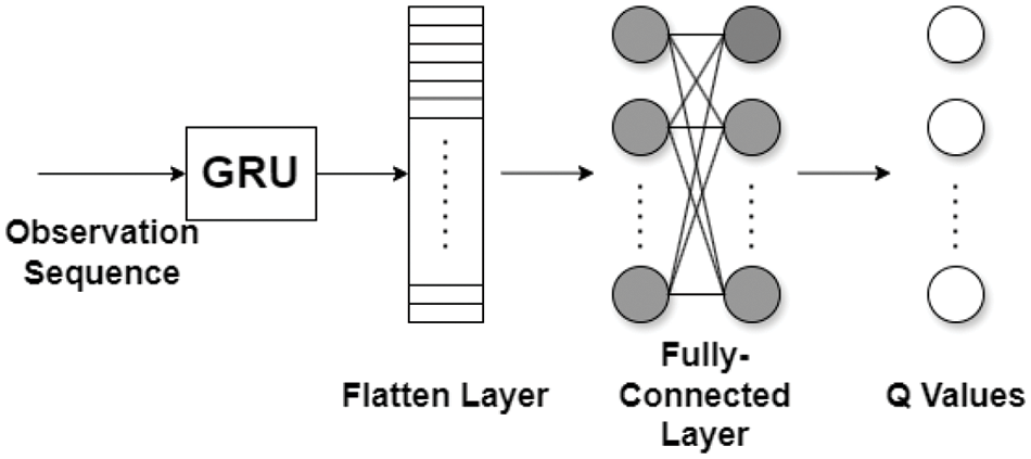
Figure 1: GRU-based DQN architecture

In POMDPs, decision-making relies on the history of observations instead of the current one [10]. We set the Q-networks to take the observation sequence as input and approximate Q values as Q(ot,at) where ot is the history of observations up to time t. Consequently, DQN used in this study consisted of two Q-networks: an evaluation Q-network Qe(ot,at,θe) and a target Q-network QT(ot,at,θT). θe and θT represent the network weights that were updated through the experience replay memory [30]. The evaluation Q-network is directly updated during the training process. It is responsible for predicting Q values, which assist in taking the action given a particular observation sequence. The target Q-network shares the same architecture as the evaluation network but operates with distinct parameters. These parameters are periodically updated by copying them from the evaluation network and remain fixed at all other times. The role of the target network is to stabilize the learning process in RL. This stabilization is crucial because Q value updates can be highly unstable, stemming from correlations between the Q value estimates and the learning targets. The target network provides stable target values for the loss function, which are used to train the evaluation network, employing an older set of parameters to compute these target Q values.

In each step of the learning process, the agent selected an action at based on the Q values predicted from the evaluation Q-network, which took the current sequence of observations ot as the input. After the agent reached the next state, it observed the environment, formed a sequence of observations ot+1, and received a reward Rt as the feedback. The experience replay, first introduced by Lin in 1992 [21], is also utilized in this study. The fundamental concept behind experience replay is to train an agent using data sampled from a buffer containing previously experienced transitions. For each transition, an experience was generated in the form of (ot,at,Rt,ot+1) and stored in a replay buffer, which is also known as a memory pool. In the meantime, a set of these experiences is selected from the memory pool to update the Q values as below and retrain the evaluation Q-network.

Qnew(ot,at)=Qe(ot,at,θe)+α[Rt+γmaxat+1QT(ot+1,at+1,θt)−Qe(ot,at,θe)](3)

where α is the learning rate. At each time step, the current transition is added to the replay buffer. The agent is then trained on a subset of transitions randomly sampled from this buffer. When the capacity of the replay buffer is reached, the oldest data is discarded to make room for the newest entries.

Differing from the value-based RL methods that solve optimal value functions, policy-based RL methods can directly find optimal policies. Proximal policy optimization (PPO) [30] is a typical policy-based method. The core concept involves parameterizing the policy itself and optimizing it directly. This category is often referred to as policy-gradient methods because they focus on adjusting policies directly through gradient descent. Conventional policy gradient methods, including advantage actor critic (A2C) [31], have demonstrated effectiveness in various decision-making scenarios. Despite facing numerous challenges in choosing the right iteration step size and optimizing data use, the PPO algorithm addresses these issues effectively. Structured under the actor-critic framework, PPO utilizes an actor network to determine actions based on specific states and a critic network to evaluate the value function that influences the performance of the actor network.

2.3 Continual Learning

This section will introduce two different continual learning algorithms: EWC [11] and Experience Replay (or Rehearsal). We chose these two algorithms because they represent two mainstream CL algorithms: regularization-based and rehearsal-based. EWC is an algorithm that mimics synaptic consolidation in artificial neural networks. It applies a quadratic penalty on the differences between parameter settings from previous tasks and new ones. This penalty slows down updates on weights that are crucial for previously acquired knowledge. When dealing with two independent tasks—an old task A with dataset DA and a new task B with dataset DB-and viewing neural network training from a probabilistic standpoint, optimizing the parameters essentially means identifying their most probable values for the entire data D=DA∪DB. This conditional probability, p(θ|D), is calculated using the prior probability of the parameters p(θ|DA) and the likelihood of the new data given the model p(DB|θ). The posterior probability can be determined by Bayes’ rule [11].

Although the true posterior probability is too complex to compute directly, EWC approximates it using a Gaussian distribution. This approximation uses the parameters θA∗ as the mean and the diagonal of the Fisher information matrix F to represent the precision, which is assumed to be diagonal. The Fisher information matrix F [32] quantifies a model’s expected sensitivity to a change in its parameters. Close to the local minimum of the loss function used in training, the matrix can be evaluated through the second-order derivatives with respect to model parameters, denoted as F=E(x,y)∼Doriginal[∇2logp(y|x;θ)]. When fine-tuning with EWC, the Fisher information is utilized to adjust the cost of updating parameters θi from the original value θA,i∗, moderated by the hyper-parameter λ. The equation is given by:

L(θ)=LB(θ)+∑iλ2Fi(θi−θA,i∗)2(4)

where LB(θ) represents the loss associated with task B, λ determines the relative importance of the old task compared to the new one, and i indicates the indices of the parameters. Thus, this method involves applying a diagonal weighting to the parameters of the learned tasks, proportional to the diagonal elements of the Fisher information matrix. The synaptic importance is calculated offline, which restricts its computational use to output spaces with lower dimensions [13].

The Rehearsal method [21] offers a distinct strategy to mitigate forgetting in models tasked with sequential learning. This approach involves retaining some previously encountered data and integrating it with new data during the training of subsequent tasks. By “rehearsing” information from earlier tasks, the model maintains familiarity with them while simultaneously learning new tasks. In our studies, we didn’t generate pseudo-data for the Rehearsal method. Specifically, the method stores a subset of data from previous tasks in a fixed-size memory (memory pool) and revisits the memorized samples during the training process for a new task. This mixed training helps the model to maintain its performance on the old tasks while adapting to new ones. To update the model, a batch sampled from the memory is combined with the incoming batch from the stream to compute the gradient.

2.4 Problem Definition and Proposed Method

This research addresses the challenge of training agricultural management RL agents that can perform effectively across various environments. We trained intelligent agents under different weather conditions, such as rising temperatures, decreasing precipitation, and historical events like the 1983 Iowa heat wave. We only employed single-agent RL in this study. Throughout the agent’s learning, we assumed that the reward function was consistent across different training environments (i.e., weather conditions), and the action space remained unchanged.

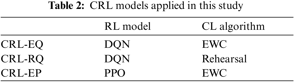
In this study, we introduced a framework that combines CL techniques with Deep Reinforcement Learning (DRL) algorithms, which we have named CRL. The core concept of this approach involves training neural networks within DRL systems using CL techniques. We examined three different CRL methods, as listed in Table 2. In the EWC-based CRL approach, we gathered the Fisher information matrix from the neural network used in DRL for the prior task. This matrix represented the importance of the weights in the neural network. Using L2 regularization, we constrained the important weights for old tasks while updating the neural network in DRL for the new task. In contrast, the Rehearsal-based CRL methods utilized data from both old and new tasks to train the agent, sourcing training data equally from all memory pools.

3  Simulation Results and Discussions

In the partially observable agricultural environment, we employed a time series of observations as inputs to neural networks in various CRL methods, as detailed in Table 1. Based on prior experimentation [9], a sequence of five timesteps was found to be optimal. For the DQN, CRL-EQ, and CRL-RQ methods, we designed Q-networks featuring a GRU layer with a single hidden layer of 64 neurons. The output from this layer was fed into a fully connected network that uses rectified linear activation functions (ReLU). The architecture of this fully connected network consists of an input layer receiving the output from the GRU, followed by one hidden layer with ReLU activation functions, and an output layer providing the Q values for action selection. The training process spanned 6000 episodes for the initial task and 3000 episodes for subsequent tasks. We utilized PyTorch and the Adam optimizer to fit our neural networks, setting an initial learning rate of 1e-5 and a batch size of 640. In the CRL-EP method, a similar GRU configuration with one hidden layer of 64 neurons was used for both actor and critic networks. The model training and testing were conducted using Python on a system equipped with an Intel Core i7-12700K processor, NVIDIA GeForce RTX 3070 Ti graphics card, and 64 GB of RAM.

3.1 Methodology Evaluations and Selections

To assess the effectiveness of the models presented in Table 2, we conducted an empirical study focusing on a historical extreme weather event—the 1983 heat wave in Iowa—which led to a 32% reduction in corn yields from the previous year [9]. This study aimed to develop an optimal agricultural management strategy (i.e., policy) that would be effective in both 1982 and 1983 despite their differing weather conditions. We employed actual weather data from these years while keeping soil data consistent with conditions from 1999. Utilizing CRL methods, we initially trained the agent using 1982 weather data until an optimal policy was established. The agent was then continually trained under 1983 weather conditions to update the optimal policy. Additionally, we trained agents separately under each year’s weather conditions to derive year-specific optimal policies. The reward functions and available actions remained identical in both scenarios, representing 1982 and 1983. Our goal was to identify the most effective CRL method from Table 2 for further applications in our study.

Initially, we evaluated the performance differences between the EWC and Rehearsal strategies, each integrated with the DQN approach in this study. These methods were labeled CRL-EQ and CRL-RQ, as outlined in Table 2. The CRL-EQ method involved first training the agent to master an optimal policy for the old task, addressing only the weather conditions of 1982. This method computed the Fisher information matrix to pinpoint critical weights within the Q-networks and then applied L2 regularization to preserve these weights. At the same time, the agent learned the new task under the 1983 weather conditions. The resulting optimal policy was denoted as 8283EQ, reflecting the integration of learnings from 1982 and 1983 using the CRL-EQ method.

Additionally, with the CRL-RQ method, once the agent was proficient with the 1982 weather conditions, we gathered the last 75,000 data samples from this task, creating Memory Pool 1. As the agent continued to learn under the 1983 weather conditions, it accumulated new data through interactions with the agricultural environment, forming Memory Pool 2. Through a first-in-first-out strategy, we maintained Memory Pool 2 to have the same amount of data as Memory Pool 1. During continual learning, the Q-networks were frequently updated by a batch of data equally selected from Memory Pools 1 and 2. The policy developed through this method was labeled 8283RQ, signifying the policy derived from learning across both 1982 and 1983 using the Rehearsal algorithm. For comparative purposes, the optimal policies developed independently under the 1982 and 1983 conditions using the DQN were designated as 1982DQN and 1983DQN, respectively. The performances of all these policies within the years 1982 and 1983 are compared separately in Fig. 2.

Figure 2: Performance comparison between optimal policies learned from DQN, CRL-EQ, and CRL-RQ methods

Fig. 2 displays the rewards obtained when various policies were applied to agricultural management in 1982 and 1983. The results for each year were normalized against the total rewards from the respective single-year policies, as shown in Fig. 2a,b. These single-year policies, such as 1982DQN and 1983DQN, were developed specifically for each year and served as ideal benchmarks for evaluating the effectiveness of the optimal policies derived from the CRL methods. Evidently, using a policy tailored for one year in a different year significantly diminishes performance. For instance, as depicted in Fig. 2b, using the policy developed for 1982 yielded only 66% of the rewards in 1983, compared to using the policy specifically learned for 1983. Correspondingly, the corn yield dropped by 35%, aligning with the reported percentage decrease due to the 1983 heat wave. This underscores the lack of adaptability in policies developed under normal conditions (like in 1982) when applied to years experiencing extreme weather conditions (such as the 1983 heatwave). A similar pattern is also noticeable in Fig. 2a, highlighting the challenges in cross-year policy application.

On the other hand, Fig. 2 clearly demonstrates that both the 8283EQ and 8283RQ policies garnered better rewards when considering both years, highlighting the robust adaptability of policies derived from the CRL methods in this context. Furthermore, the 8283EQ policy overall outperformed the 8283RQ policy, especially in 1982, although the agent collected slightly fewer rewards in 1983 by following the 8283EQ policy than the 8283RQ policy. This underscores the superior performance of the EWC algorithm in DQN compared to the Rehearsal algorithm. The discrepancy arises due to limited computing and storage resources, which prevent us from providing a larger Memory Pool for the CRL model utilizing the Rehearsal algorithm. Memory Pool 2 was frequently updated as the agent learned new tasks using the CRL-RQ method, whereas Memory Pool 1 remained unchanged as it contained only a limited amount of data from an older task.

As a result, the optimal policy achieved performed better in the new task of 1983 than in the old task of 1982. In contrast, the EWC algorithm managed to learn new skills while retaining most of the old knowledge by constraining some network weights through the Fisher information matrix. It shall be noted that implementing the Rehearsal algorithm in the DQN method made the CRL-RQ method converge faster than the CRL-EQ method, but it tended to forget previously learned information more rapidly. Although Rehearsal can often achieve similar or even superior performance compared to EWC, this study is conducted in a resource-constrained environment with limited computational resources. As the number of tasks increases, Rehearsal requires managing and potentially retraining on a larger volume of data, which escalates computational demands. Consequently, EWC delivers better performance and is preferred in this study due to its lower computational and storage demands.

The discussion above suggested that EWC was a more effective continual learning algorithm than Rehearsal when implemented in the value-based RL method, DQN. We then evaluated the performance of the CRL-EP method (as listed in Table 2), which applied EWC within a policy-based RL method, PPO. In the case of DQN, collecting the Fisher information matrix from a single Q-network suffices after learning from the old task, as the target Q-network shares the same architecture and weights as the evaluation Q-network. However, for the CRL-EP method, it is essential to gather the Fisher information matrices for both the actor and critic networks after the old task is completed and then apply these matrices to the respective networks for the new task. The policy developed through this approach was labeled 8283EP and was compared against other policies in Fig. 3. Our findings revealed that the 8283EQ policy consistently outperformed the 8283EP policy by 4%–5%. Based on these results, we decided to continue with the CRL-EQ model for future research, as it has demonstrated superior performance in our evaluations.

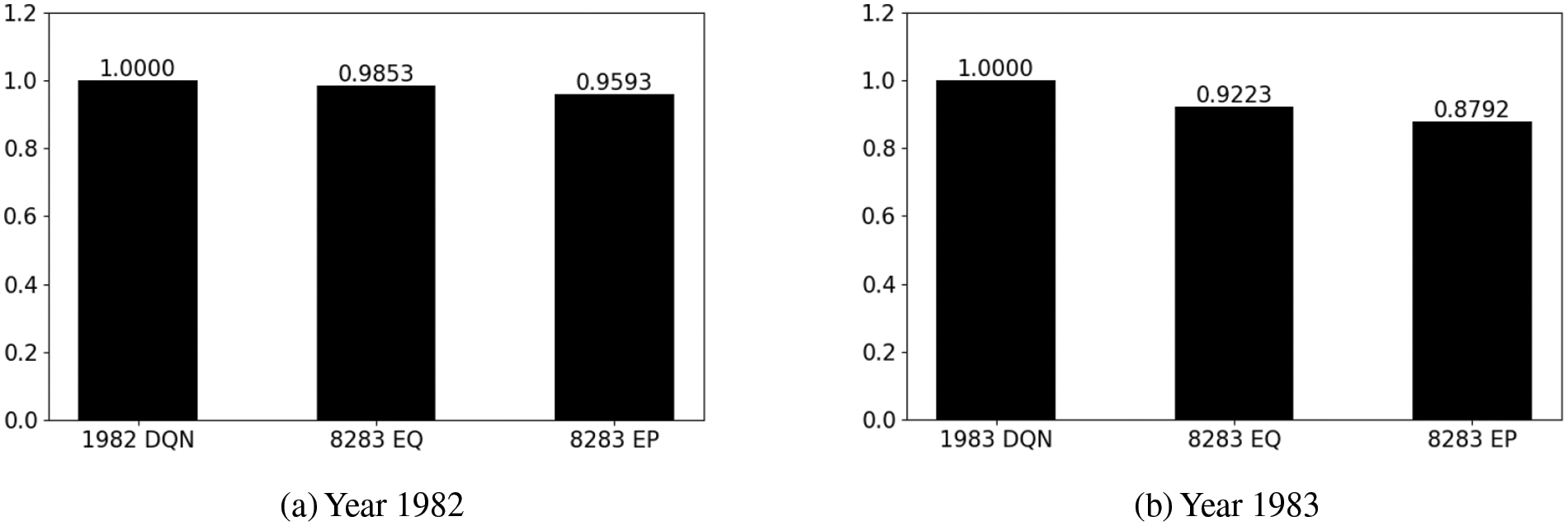
Figure 3: Performance comparison between optimal policies learned from DQN, CRL-EQ, and CRL-EP methods

3.2 Climate Variabilities

In our subsequent study, we used 1999 weather data as a baseline, introducing variations in temperature and precipitation to assess the performances of CRL policies under more than two climate variability conditions. We conducted two scenarios: a temperature increase and a precipitation decrease. In the first scenario, we incrementally raised the daily average temperature from the 1999 baseline by 1, 2, 3, 4, and 5 degrees Celsius throughout the year while maintaining the precipitation levels as in 1999. In the second scenario, we reduced daily rainfall by 20%, 35%, 50%, 65%, and 80% over the course of the year, keeping temperature patterns consistent with those of 1999. It is important to note that the soil data for all simulations remained consistent with 1999 conditions. Additionally, this study did not address scenarios of increased precipitation potentially leading to flood-related crop damage, as these conditions are beyond the predictive capabilities of the DSSAT.

This study examined three types of policies: fixed policy, optimal policies, and policies derived through the CRL method. The fixed policy replicated the optimal policy learned using actual 1999 weather data and remained unchanged, even under hotter or drier conditions. In contrast, the agent was trained to learn new optimal policies as weather conditions varied, adjusting the agent in response to climatic changes such as increases in temperature or decreases in rainfall. Additionally, we employed the CRL-EQ method to train the agent sequentially under various weather changes, ultimately deriving the final policies. There were six tasks in the temperature rise scenario, spanning adjustments from +0 to +5 degrees Celsius. After training the agent under each task, the EWC algorithm calculated the Fisher information matrix and applied regularization to the important weights of Q-networks while adapting to another new task. A similar approach was used in the rainfall decrease scenario. The final policies were named EQT for temperature scenarios and EQP for scenarios involving precipitation reduction from 0% to 80%. Overall, EQT represents the CRL policy developed to manage rising temperatures, trained specifically under scenarios of increasing temperature. On the other hand, EQP is the CRL policy tailored to address changes in precipitation and is trained under varying precipitation conditions. The role of EQT and EQP policies in studying climate variability is to demonstrate that those policies from the CRL method exhibit more robust capabilities to adapt to climate changes, particularly under conditions of significant variability.

Fig. 4 compares the performance of various policies under conditions of rising temperatures. Each optimal policy, tailored to specific weather conditions, served as the most effective agricultural management strategy for those conditions. The rewards collected by following each optimal policy were normalized to a baseline of 1, with the performances of other policies scaled accordingly. Initially, the fixed policy outperformed the EQT policy by a narrow margin of about 3%, showcasing the adaptability of both policies to minor temperature increases. However, as the average temperature increased by 2 degrees Celsius, the EQT policy began to show superior performance. The performance gap widened to 26.5% when the temperature rise reached 5 degrees Celsius. This highlighted how the EQT policy significantly outperformed the fixed policy under more severe high-temperature conditions, emphasizing its potential in adapting to future climate change scenarios.

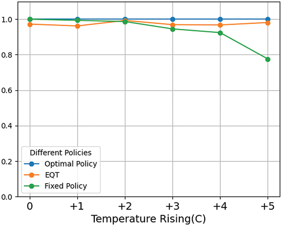
Figure 4: Comparison of different policies when temperature rises

Fig. 5 presents the comparative performance of each policy under scenarios of decreasing precipitation. The results demonstrate that the EQP policy consistently outperformed the fixed policy across all levels of precipitation reduction, particularly under conditions of significant rainfall decrease. For instance, when precipitation was reduced by 80%, the EQP maintained 92.6% of the baseline performance, while the fixed policy achieved only 37%. This stark contrast highlights the EQP’s superior performance under extreme rainfall reduction conditions. These findings reinforce our earlier conclusions regarding the impact of climate variability on agriculture and agricultural management. While the fixed policy, learned under normal weather conditions, shows some adaptability to minor climatic variations, policies developed using the CRL method exhibited robust and stable performance even in extreme weather conditions.

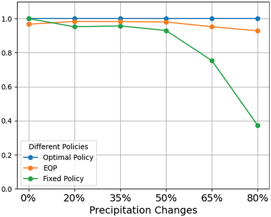
Figure 5: Comparison of different policies when precipitation reduces

3.3 Weather Uncertainty

We further assessed the performance of continually learned policies (EQT and EQP) alongside the fixed policy under conditions of weather uncertainty, expanding on previous discussions. For this study, we utilized 1999 weather data as the base sample and employed WGEN [33], a stochastic weather generator, to create random weather events. We ensured consistent conditions across simulations of different policies by using the same “random seed.” This approach guaranteed that, when simulating policies under identical weather events (e.g., average temperature +1°C), each policy was tested with 100 simulations, and the size and sequence of the 100 sets of weather data generated by WGEN remained the same for each policy. After collecting simulation data from all policies, we calculated the mean reward, corn yield, total nitrogen inputs, and nitrate leaching based on the 100 simulations under specific weather events. We then established the performance of the fixed policy as the baseline against which we compared the performances of various other policies.

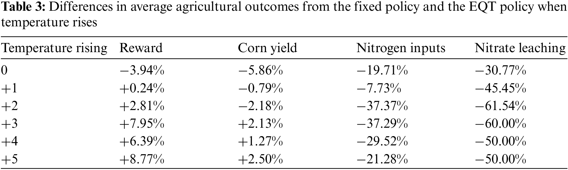
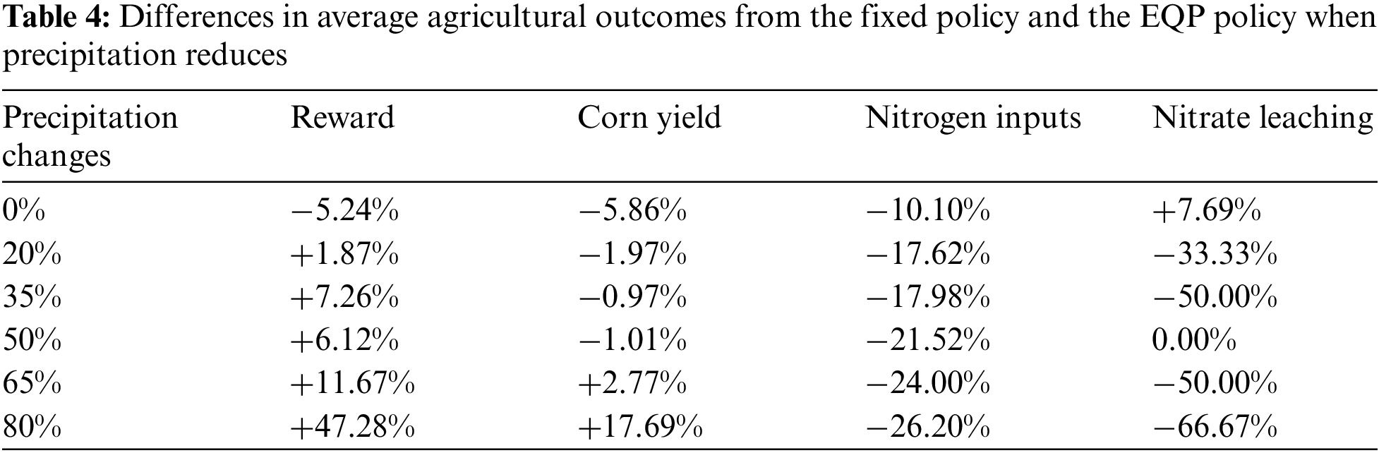
Tables 3 and 4 compare the average agricultural outcomes, including total reward, corn yield, nitrogen inputs, and nitrate leaching, between the continually learned and fixed policies under temperature-rising and precipitation reduction scenarios. In the first scenario, the values in ‘Temperature Rising’ indicate increases in monthly maximum and minimum temperatures. In the second scenario, the percentages in ‘Precipitation Changes’ reflect reductions in monthly average rainfall rather than daily variations. The metric we used was the relative differences in the outcomes between the continually learned and fixed policies, while the outcomes from the fixed policy were the baselines.

In the first scenario, monthly maximum and minimum temperatures were increased by up to 5 degrees Celsius, and daily temperatures were randomly generated with varying patterns. This approach differed from our earlier study in Section 3.2, where the temperature patterns were fixed to replicate those from 1999. Importantly, while daily rainfall was also generated randomly using WGEN, the total monthly precipitation levels remained consistent with those observed in 1999.

Table 3 compares the average agricultural outcomes between the continually learned policy (EQT) and the fixed policy at various temperature rises. In this table, the fixed policy slightly outperformed the EQT policy under normal temperature (+0°C) in terms of total reward and corn yield. However, the EQT policy effectively reduced nitrogen fertilizer usage by 19.71%, subsequently decreasing nitrate leaching by 30.77%. With temperature increases of 1°C and 2°C, corn yields from the EQT policy were lower. However, due to lower nitrogen inputs and nitrate leaching, the EQT policy achieved higher total rewards than the fixed policy. Furthermore, as temperatures continued to rise, the EQT policy consistently outperformed the fixed policy. At temperature increases of 3°C and above, the EQT policy’s performance was superior to that of the fixed policy. The largest difference occurred at a temperature increase of 5°C, where the EQT policy achieved an 8.77% higher total reward, a 2.5% higher corn yield, a 21.28% reduction in nitrogen input, and a 50% reduction in nitrate leaching compared to the fixed policy.

The second scenario involved reductions in monthly (rather than daily) average rainfall by 20%, 35%, 50%, 65%, and 80%. Similarly, daily temperatures were randomly generated, but the monthly maximum, minimum, and average temperatures aligned with the 1999 weather data.

Table 4 provides a comparison of the average agricultural outcomes between the continually learned policy (EQP) and the fixed policy under varying precipitation reduces. Initially, under the same precipitation levels as in 1999, the EQP policy generally underperformed in corn yield compared to the fixed policy but had better performance in reducing nitrogen inputs. This was because the fixed policy was learned specifically under normal weather, and it was expected to perform the best. However, as rainfall decreased, the EQP policy consistently outperformed the fixed policy. With precipitation reductions up to 50%, the EQP policy achieved a higher total reward than the fixed policy by maintaining similar corn yields while using less nitrogen fertilizer and reducing nitrate leaching. When precipitation was reduced by 65%, the EQP policy produced higher yields, utilized less nitrogen, and resulted in less nitrate leaching than the fixed policy. Notably, when precipitation reached 80% less than normal, the EQP policy demonstrated a significant performance improvement of 47.3% over the fixed policy. Echoing findings from Table 3, under dramatic climate changes, the continually learned policy not only matched or exceeded corn yields from the fixed policy but also reduced nitrogen usage, thereby minimizing environmental impacts such as nitrate leaching.

4  Conclusion and Future Works

Developing a management strategy (i.e., policy) that can adapt to a wide range of climate conditions poses a significant challenge in agricultural management. Current RL approaches often struggle to adjust to varying weather patterns, leading to suboptimal outcomes under extreme weather conditions. This research addresses the challenge by integrating the strengths of RL and CL, allowing agents to learn highly adaptable policies.

Specifically, we developed a framework incorporating CL algorithms and RL methods to create CRL methods, demonstrating their implementation and evaluation utilizing Gym-DSSAT. Throughout the exploration of various RL and CL combinations, we found that integrating EWC with DQN yielded superior results. We further assessed the model’s adaptability by considering climate variability, including increased temperatures and reduced precipitation. Our findings showed that policies learned through the CRL method exhibited enhanced adaptability compared to pre-established optimal policies, particularly in scenarios of decreased rainfall. Moreover, by incorporating WGEN, a stochastic weather generator, into our crop simulation framework, we generated variable weather patterns based on real data, thereby expanding our evaluation of the model’s robustness against weather uncertainty.

The results indicate that while previously established policies could manage mild variations in temperature and precipitation effectively, they struggled under severe conditions, such as drastic reductions in rainfall or droughts. In contrast, CRL-based policies, learned across multiple tasks corresponding to different weather conditions in this study, demonstrate greater adaptability, especially in response to extreme climatic events. Compared to models developed in prior research, our approach enhances adaptability within a similar time frame and dataset. This advancement holds promise to significantly improve the versatility of our model and inspire new strategies in future agricultural management.

Moving forward, enriching datasets beyond those from 1999, particularly the soil properties data, will be crucial to further testing and verifying the performance of policies learned from our proposed CRL methods. Additionally, since this test is based on conditions in Iowa, which is a rain-fed state, the effect of irrigation has been overlooked. Consequently, this study focuses on fertilization management. Therefore, we plan to investigate agricultural management with fertilization and irrigation in future studies. It would be ideal to implement the learned policies in the testing field under actual weather conditions. We believe that with minor modifications, the framework developed in this study can be effectively adapted for agricultural irrigation management, significantly enhancing the real-world applicability of our research in agricultural settings.

This framework will also prove highly beneficial in other fields, such as robotics. Although one study [25] has been reported employing EWC and DDPG in robotics, they only considered simple go-to-goal motion planning tasks in fully observation environments. In our future work, we will apply the developed CRL framework to robotics problems involving complex tasks and partially observable environments [34,35], aiming to tackle more intricate challenges. This expansion will broaden our framework’s scope and demonstrate its adaptability and effectiveness across different fields.

Although our CRL method produces highly adaptable policies, our implementation with EWC, which is the primary focus of this paper, encounters certain limitations. In this study, we employed the same reward function across different environments. To extend our framework for more general applications in which the reward functions vary at different environments, the Fisher information matrix needs to be carefully redesigned. Specifically, the naïve Fisher information matrix struggles to accurately measure the model’s sensitivity to parameter changes from the previous task in new environments where these parameters will respond differently to the new reward function. This makes it challenging to train a model capable of simultaneously adapting to diverse tasks. Another limitation arises when applying our approach to multi-agent RL, where individual agents would require distinct Fisher information matrices, potentially complicating subsequent training. Alternatively, using the Rehearsal method may simplify this issue. As we look to future research, particularly in multi-agent CRL, our focus will shift towards integrating Rehearsal techniques with RL to address these complexities.

Acknowledgement: Not applicable.

Funding Statement: Zhaoan Wang and Shaoping Xiao received support from the University of Iowa OVPR Interdisciplinary Scholars Program and the US Department of Education (ED #P116S210005) for this study. Kishlay Jha’s work is supported in part by the US National Institute of Health (NIH) and National Science Foundation (NSF) under grants R01LM014012-01A1 and ITE-2333740. Any opinions, findings, conclusions or recommendations expressed in this material are those of the authors and do not necessarily reflect the views of funding agencies.

Author Contributions: Study conception and design: Zhaoan Wang, Kishlay Jha, Shaoping Xiao; data collection: Zhaoan Wang; analysis and interpretation of results: Zhaoan Wang, Shaoping Xiao; draft manuscript preparation: Zhaoan Wang, Kishlay Jha, Shaoping Xiao. All authors reviewed the results and approved the final version of the manuscript.

Availability of Data and Materials: Not applicable.

Ethics Approval: Not applicable.

Conflicts of Interest: The authors declare that they have no conflicts of interest to report regarding the present study.

References

1. N. Zhang, M. Wang, and N. Wang, “Precision agriculture—A worldwide overview,” Comput. Electron. Agric., vol. 36, no. 2, pp. 113–132, Nov. 2002. doi: 10.1016/S0168-1699(02)00096-0. [Google Scholar] [CrossRef]

2. L. P. Kaelbling, M. L. Littman, and A. W. Moore, “Reinforcement learning: A survey,” J. Artif. Intell. Res., vol. 4, pp. 237–285, May 1996. doi: 10.1613/jair.301. [Google Scholar] [CrossRef]

3. M. Cai, S. Xiao, J. Li, and Z. Kan, “Safe reinforcement learning under temporal logic with reward design and quantum action selection,” Sci. Rep., vol. 13, no. 1, Feb. 2023, Art. no. 1925. doi: 10.1038/s41598-023-28582-4. [Google Scholar] [PubMed] [CrossRef]

4. J. Li, M. Cai, Z. Wang, and S. Xiao, “Model-based motion planning in POMDPs with temporal logic specifications,” Adv. Robot, vol. 37, no. 14, pp. 871–886, Jul. 2023. doi: 10.1080/01691864.2023.2226191. [Google Scholar] [CrossRef]

5. R. Gautron, E. J. Padrón, P. Preux, J. Bigot, O. -A. Maillard and D. Emukpere, “gym-DSSAT: A crop model turned into a reinforcement learning environment,” Sep. 27, 2022. doi: 10.48550/arXiv.2207.03270. [Google Scholar] [CrossRef]

6. J. W. Jones et al., “The DSSAT cropping system model,” Eur. J. Agron., vol. 18, no. 3, pp. 235–265, Jan. 2003. doi: 10.1016/S1161-0301(02)00107-7. [Google Scholar] [CrossRef]

7. J. Wu, R. Tao, P. Zhao, N. F. Martin, and N. Hovakimyan, “Optimizing nitrogen management with deep reinforcement learning and crop simulations,” Apr. 21, 2022. doi: 10.1109/CVPRW56347.2022.00178. [Google Scholar] [CrossRef]

8. L. Sun, Y. Yang, J. Hu, D. Porter, T. Marek and C. Hillyer, “Reinforcement learning control for water-efficient agricultural irrigation,” in 2017 IEEE Int. Symp. Parallel Distrib. Process. Appl. 2017 IEEE Int. Conf. Ubiquitous Comput. Commun. (ISPA/IUCC), Guangzhou, China, Dec. 2017, pp. 1334–1341. doi: 10.1109/ISPA/IUCC.2017.00203. [Google Scholar] [CrossRef]

9. Z. Wang, S. Xiao, J. Li, and J. Wang, “Learning-based agricultural management in partially observable environments subject to climate variability,” Jan. 02, 2024. doi: 10.48550/arXiv.2401.01273. [Google Scholar] [CrossRef]

10. Z. Wang, S. Xiao, J. Wang, A. Parab, and S. Patel, “Intelligent agricultural management considering N2O emission and climate variability with uncertainties,” Feb. 13, 2024. doi: 10.2139/ssrn.4742674. [Google Scholar] [CrossRef]

11. J. Kirkpatrick et al., “Overcoming catastrophic forgetting in neural networks,” Proc Natl. Acad. Sci., vol. 114, no. 13, pp. 3521–3526, Mar. 2017. doi: 10.1073/pnas.1611835114. [Google Scholar] [PubMed] [CrossRef]

12. G. M. van de Ven and A. S. Tolias, “Generative replay with feedback connections as a general strategy for continual learning,” Apr. 17, 2019. doi: 10.48550/arXiv.1809.10635. [Google Scholar] [CrossRef]

13. G. I. Parisi, R. Kemker, J. L. Part, C. Kanan, and S. Wermter, “Continual lifelong learning with neural networks: A review,” Neural Netw., vol. 113, pp. 54–71, May 2019. doi: 10.1016/j.neunet.2019.01.012. [Google Scholar] [PubMed] [CrossRef]

14. B. Liu, “Lifelong machine learning: A paradigm for continuous learning,” Front. Comput. Sci., vol. 11, no. 3, pp. 359–361, Jun. 2017. doi: 10.1007/s11704-016-6903-6. [Google Scholar] [CrossRef]

15. J. Kim, Y. Ku, J. Kim, J. Cha, and S. Baek, “VLM-PL: Advanced pseudo labeling approach for class incremental object detection via vision-language model,” May 08, 2024. doi: 10.48550/arXiv.2403.05346. [Google Scholar] [CrossRef]

16. F. Girosi, M. Jones, and T. Poggio, “Regularization theory and neural networks architectures,” Neural Comput., vol. 7, no. 2, pp. 219–269, Mar. 1995. doi: 10.1162/neco.1995.7.2.219. [Google Scholar] [CrossRef]

17. F. Zenke, B. Poole, and S. Ganguli, “Continual learning through synaptic intelligence,” in Proc. 34th Int. Conf. Mach. Learn., PMLR. Jul. 2017, pp. 3987–3995. Accessed: Jun. 16, 2024. [Online]. Available: https://proceedings.mlr.press/v70/zenke17a.html [Google Scholar]

18. S. -W. Lee, J. -H. Kim, J. Jun, J. -W. Ha, and B. -T. Zhang, “Overcoming catastrophic forgetting by incremental moment matching,” in Adv. Neural Inform. Process. Syst., Curran Associates, Inc., 2017. Accessed: Jun. 16, 2024. [Online]. Available: https://proceedings.neurips.cc/paper/2017/hash/f708f064faaf32a43e4d3c784e6af9ea-Abstract.html [Google Scholar]

19. Z. Li and D. Hoiem, “Learning without forgetting,” IEEE Trans. Pattern Anal. Mach. Intell., vol. 40, no. 12, pp. 2935–2947, Dec. 2018. doi: 10.1109/TPAMI.2017.2773081. [Google Scholar] [PubMed] [CrossRef]

20. A. Gupta, V. Kumar, C. Lynch, S. Levine, and K. Hausman, “Relay policy learning: Solving long-Horizon tasks via imitation and reinforcement learning,” Oct. 25, 2019. doi: 10.48550/arXiv.1910.11956. [Google Scholar] [CrossRef]

21. L. -J. Lin, “Self-improving reactive agents based on reinforcement learning, planning and teaching,” Mach. Learn., vol. 8, no. 3, pp. 293–321, May 1992. doi: 10.1007/BF00992699. [Google Scholar] [CrossRef]

22. D. Lopez-Paz and M. A. Ranzato, “Gradient episodic memory for continual learning,” in Adv. Neural Inform. Process. Syst., Curran Associates, Inc., 2017. Accessed: Jun. 16, 2024. [Online]. Available: https://proceedings.neurips.cc/paper/2017/hash/f87522788a2be2d171666752f97ddebb-Abstract.html [Google Scholar]

23. B. Maschler, H. Vietz, N. Jazdi, and M. Weyrich, “Continual learning of fault prediction for turbofan engines using deep learning with elastic weight consolidation,” in 2020 25th IEEE Int. Conf. Emerg. Technol. Factory Autom. (ETFA), Vienna, Austria, Sep. 2020, pp. 959–966. doi: 10.1109/ETFA46521.2020.9211903. [Google Scholar] [CrossRef]

24. J. -L. Shieh et al., “Continual learning strategy in one-stage object detection framework based on experience replay for autonomous driving vehicle,” Sensors, vol. 20, no. 23, Jan. 2020, Art. no. 23. doi: 10.3390/s20236777. [Google Scholar] [PubMed] [CrossRef]

25. N. Wang, D. Zhang, and Y. Wang, “Learning to navigate for mobile robot with continual reinforcement learning,” in 2020 39th Chinese Control Conf. (CCC), Shenyang, China, IEEE, Jul. 2020, pp. 3701–3706. doi: 10.23919/CCC50068.2020.9188558. [Google Scholar] [CrossRef]

26. D. Abel, A. Barreto, B. Van Roy, D. Precup, H. P. Van Hasselt and S. Singh, “A definition of continual reinforcement learning,” Adv Neural Inf. Process. Syst., vol. 36, pp. 50377–50407, Dec. 2023. [Google Scholar]

27. C. J. C. H. Watkins and P. Dayan, “Q-learning,” Mach. Learn., vol. 8, no. 3, pp. 279–292, May 1992. doi: 10.1007/BF00992698. [Google Scholar] [CrossRef]

28. K. Cho et al., “Learning phrase representations using RNN encoder-decoder for statistical machine translation,” Sep. 02, 2014. doi: 10.3115/v1/D14-1. [Google Scholar] [CrossRef]

29. V. Mnih et al., “Playing Atari with deep reinforcement learning,” Dec. 19, 2013. doi: 10.48550/arXiv.1312.5602. [Google Scholar] [CrossRef]

30. J. Schulman, F. Wolski, P. Dhariwal, A. Radford, and O. Klimov, “Proximal policy optimization algorithms,” Aug. 28, 2017. doi: 10.48550/arXiv.1707.06347. [Google Scholar] [CrossRef]

31. Z. Wang et al., “Sample efficient actor-critic with experience replay,” Jul. 10, 2017. doi: 10.48550/arXiv.1611.01224. [Google Scholar] [CrossRef]

32. J. Thorne and A. Vlachos, “Elastic weight consolidation for better bias inoculation,” Feb. 4, 2021. doi: 10.18653/v1/2021.eacl-main. [Google Scholar] [CrossRef]

33. A. Soltani and G. Hoogenboom, “A statistical comparison of the stochastic weather generators WGEN and SIMMETEO,” Clim. Res., vol. 24, no. 3, pp. 215–230, Sep. 2003. doi: 10.3354/cr024215. [Google Scholar] [CrossRef]

34. J. Li, M. Cai, and S. Xiao, “Reinforcement learning-based motion planning in partially observable environments under ethical constraints,” AI Ethics, Mar. 2024. doi: 10.1007/s43681-024-00441-6. [Google Scholar] [CrossRef]

35. J. Li, M. Cai, Z. Kan, and S. Xiao, “Model-free motion planning of autonomous agents for complex tasks in partially observable environments,” Apr. 30, 2023. doi: 10.21203/rs.3.rs-2856026/v1. [Google Scholar] [CrossRef]