Graph Attention Residual Network Based Routing and Fault-Tolerant Scheduling Mechanism for Data Flow in Power Communication Network

1  Introduction

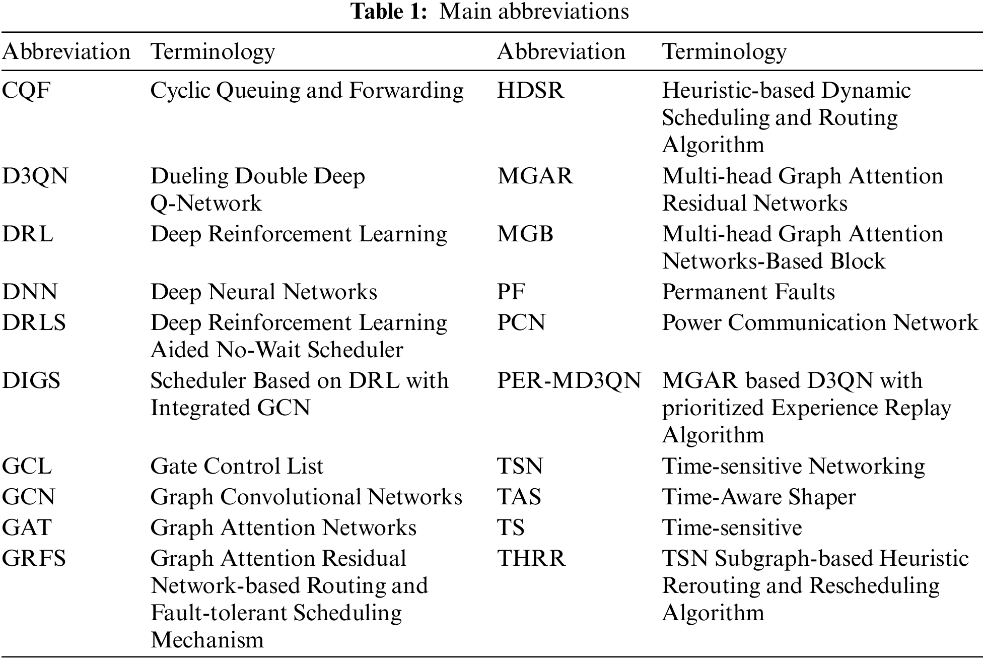
With the continuous development of smart grid technology, the role of the power communication network in the power system is becoming increasingly prominent. In this context, the distribution areas of the power communication network collect data, monitor, and control operations through intelligent integrated terminals, achieving communication and data exchange with the master station system. Intelligent integrated terminals, installed in low-voltage distribution areas, are responsible for high real-time and high-reliability functions such as data collection, equipment monitoring, and control operations, providing strong support for the stable operation of the power system. As the volume of data transmission in the power system continues to increase, the real-time and reliable communication between integrated terminals increasingly relies on the low latency and high jitter resistance communication services provided by the Time-Sensitive Networking (TSN) based on global clock synchronization, Time-Aware Shaper (TAS), and Cyclic Queuing and Forwarding (CQF) [1]. However, in practical situations, TSN may not be able to ensure the sustainability of communication services due to equipment failures, link interruptions, etc., leading to serious negative impacts on the power data communication network due to prolonged data loss for time-sensitive integrated terminal communication. Therefore, to ensure the stability and reliability of the communication services provided by TSN for integrated terminals, the routing scheduling mechanism needs to have fault-tolerance ability (The main abbreviations of terminology are detailed in Table 1).

The fault-tolerant routing and scheduling mechanism of TSN, when facing permanent faults (PF) such as node failures and link interruptions, mainly provides protection through two methods: (i) Path Protection: Space redundancy is used to allocate two non-intersecting paths for each connection, i.e., the primary path and the backup path. (ii) Link Protection: Finding alternative links during the fault to take over the rerouted traffic [2], i.e., a rapid rerouting fault recovery fault-tolerance method. Regarding path protection, the scheduling mechanism usually implements space-redundant multi-path transmission of multiple data replicas using heuristic algorithms, Integer Linear Programming (ILP), and Satisfiability Modulo Theories (SMT) [3–7]. And the methods may be applied in combination in path protection to improve efficiency, such as heuristic algorithms and ILP [8]. Besides path protection often needs to work together with the IEEE 802.1CB mechanism for frame replication and elimination [9,10]. But path protection requires lots of time to pre-calculate candidate paths to build its redundant path set and occupies multiple network resources, resulting in low effective utilization and affecting the upper limit of normal scheduling performance [11]. Even by pre-calculating and storing to minimize response time, the methods of path protection have to occupy network resources multiply and are still essentially static, only fault-tolerant for small-scale closed networks with known, pre-calculated redundant paths for expected permanent faults [12]. Moreover, in the complex and dynamic TSN, there is a situation where link failures occur on all limited redundant transmission paths [2]. So in the online scenario that requires incremental scheduling, TSN usually provides link protection for rerouting and scheduling of traffic related to faulty node links as a trade-off between fault-tolerance and scheduling performance [13–15]. However, using methods such as ILP and SMT to recover the transmission of many TS flows still requires a long response time. To alleviate this issue, methods such as topology pruning [16] and limiting the number of candidate paths [17] are commonly adopted for time cost optimization, but they fail to fully utilize routing information to optimize fault-tolerance, neglecting feasible solutions to flows in fault.

Therefore, the static redundant path fault tolerance method of path protection has problems such as long computation time, low effective utilization of resources, and limited fault tolerance capability for multi-point faults, while the link protection fault-tolerance method of rerouting scheduling has the problem of long response time when the scale of TS traffic is large. Deep Reinforcement Learning (DRL), which can interact and learn from complex environments without too much simplification, provides a new approach for rapid response to the highly dynamic TSN and has achieved good scheduling performance in fault-free ideal states [18]. So DRL could respond quickly to the feasible fault recovery solution without reducing the scale of the problem.

But facing the network data with the graph structure, especially in the case of topology changes caused by node-link failures, the scheduling mechanism implemented by Deep Neural Networks (DNN) [19] or Graph Convolutional Networks (GCN) [20] still has certain shortcomings. GCN has an over-smoothing issue where node features tend to homogenize with network depth, and indiscriminately aggregate node features, which can lead to the influence of anomalous node link features on the effectiveness of decision-making. But Graph Attention Networks (GAT) can adjust inter-node data weights based on traffic transmission task requirements and selectively fuse weighted data and GAT proximal policy optimization algorithm [21] achieves better scheduling performance than GCN-DRL. Besides, GAT have been utilized as the centralized critic in the actor-critic algorithm, assisting in addressing the distributed scheduling issues in the integration of 5G with TSN [22].

However, GAT face the over-smoothing issue also. And the DRLs with GAT used in TSN above [21,22], do not consider improvement for fault-tolerance, such as the combination of routing and scheduling that finds more feasible solutions in multipath, and load balancing that controls the loss caused by link fault and reserves resources for rerouting and rescheduling.

In addition, most TS flow scheduling mechanisms with fault-tolerance capabilities consider TSN based on TAS. TAS can achieve wait-free packet scheduling, but the bandwidth utilization rate is low, and the allocation of time slots for each packet requires complex computation and configuration of the Gate Control List (GCL) [23]. Therefore, the algorithm for rerouting and scheduling faulty TS flows based on the TAS model obviously requires a longer response time, and there are fewer solutions that can meet the requirements without changing the GCL of other TS flows. Although CQF has a larger jitter, it simplifies the configuration of the GCL compared to TAS and can use a lightweight heuristic algorithm to schedule the injection time slots of TS flows [24,25]. CQF can achieve better resource utilization and load balancing effects on the transmission path, thus having better application prospects in reducing the impact of faults and increasing the number of reroutable TS flows.

To address the issues, this paper studies the fault-tolerant scheduling problem of TS flows in TSN and proposes a graph attention residual network-based routing and fault-tolerant scheduling mechanism for data flow in the power communication network distribution area (GRFS), with specific contributions as follows:

1) A communication system architecture for integrated terminals based on CQF and fault recovery method is designed. This architecture reduces the complexity of the routing scheduling algorithm and the impact of permanent faults on the solution by using CQF with simple scheduling configuration and adopts a fault recovery method that prioritizes the rerouting of faulty traffic. CQF and fault recovery used in the architecture improve the upper limit of system performance under ideal states and avoid frequent expansion and change of TSN as the power data communication network develops.

2) An optimization model for the joint routing and scheduling problem is established. The model aims for a higher scheduling success rate, with traffic latency and network load as constraints. The model finds more feasible solutions in the network with topological changes by gradually specifying the routing and injection time slot range and reduces the faulty TS flows caused by PF by controlling the network load instead of mandatory resource reservation, thereby increasing the upper limit of the ideal state scheduling success rate and objectively reserving resources for the rerouting of faulty TS flows.

3) A multi-head graph attention residual network (MGAR) based Dueling Double Deep Q-Network (D3QN) with prioritized experience replay algorithm (PER-MD3QN) is constructed. PER-D3QN uses the MGAR encoder to reconstruct the TSN state, traffic features to obtain feature embedding vectors, and the dueling network decoder to decode the feature embedding vectors into decisions. So, PER-MD3QN flexibly adjusts the weights through the attention mechanism of MGAR, selects the relatively key information from the characteristics of the current task in the various input TSN and traffic, and finds routes with legal injection time slots for the TS flow.

The rest of this paper is organized as follows. Section 2 introduces the related works. Section 3 introduces the communication system architecture for integrated terminals based on CQF and fault recovery methods. Section 4 introduces the optimization model for joint routing and scheduling designed for the TSN scenario with node-link failures, aiming to maximize the scheduling success rate of TS flows. In Section 5, the design of the D3QN algorithm based on MGAR to reconstruct the TSN state and traffic features, and then decoded by a multi-layer perceptron, is detailed. Section 6 provides simulation and result analysis. Finally, conclusions are drawn in Section 7.

2  Related Works

The challenges to the reliability and sustainability of TSN networks can be broadly categorized into two types: temporary faults and permanent faults. Temporary faults, primarily caused by bit flips, result in data frame errors, which are typically addressed through time redundancy by sending multiple copies of the same data over the same link [26]. However, given the heightened sensitivity of power communication networks to scenarios involving permanent node or link failures, this paper primarily focuses on permanent fault issues. In response to permanent node or link failures, Balasubramanian et al. [2] employed a TSN controller based on federated learning, considering multiple paths with the lowest joint failure probability to provide protection, thereby minimizing the risk of tolerance failure due to multi-point faults. Pahlevan et al. [3] based on heuristic algorithms and proposed a fault-tolerant list scheduler for time-triggered communication in TSN. Syed et al. [4] developed a fault-tolerant dynamic scheduling and routing approach. Dobrin et al. [5] explored fault-tolerant scheduling in time slot sensitive networks, providing insights for the security and dependability of critical embedded systems. Zhou et al. [6] presented a reliability-aware scheduling and routing strategy for TSN networks, increasing the network’s fault-tolerance. Zhou et al. [7] proposed an ASIL-decomposition-based approach for routing and scheduling in safety-critical TSN networks, addressing the challenges of high-integrity applications. Chen et al. [8] used ILP and introduced a meta-heuristic-based method for multipath joint routing and scheduling of time-triggered traffic in TSN for IIoT applications. Atallah et al. [9] investigated routing and scheduling for time-triggered traffic in TSN, advancing the understanding of industrial network communication. Chen et al. [10] suggested a heuristic-based dynamic scheduling and routing method for industrial TSN networks, aiming to enhance network efficiency. Feng et al. [11] proposed a method that combines temporal redundancy protection across multiple disjoint paths with online rerouting and scheduling for link protection, supplementing failed paths caused by permanent faults. However, the method in [11] inevitably requires more resources than static redundancy paths. As the rapidly evolving power communication networks face escalating communication demands among converged terminals, spatially redundant path protection methods as mentioned may necessitate frequent expansion and adjustment due to resource redundancy limitations.

Recognizing the negative impact of static spatial redundancy on scheduling performance, Kong et al. [13] introduced a dynamic redundancy approach for rerouting failed TS flows, leveraging SDN architecture and ILP solvers. This method boasts lower bandwidth redundancy requirements and effective protection against multi-point faults. Nandha Kumar et al. [14] utilized heuristic algorithms to identify the minimal connected subgraph for isolating problem areas, minimizing the solution time for traffic rerouting in the affected network segments. Bush [27] pointed out that preconfiguring or storing scheduling for every possible network fault in resource-constrained and dynamically changing TSNs is infeasible, introducing the concept of processing-storage trade-off through scheduling seeds and utilizing SMT to solve polymorphic reconfiguration scheduling under resource constraints. Nevertheless, methods based on ILP, SMT, and heuristic algorithms experience increased average computation time as network and traffic scales grow. Although seamless redundancy may not always be necessary for industrial communication networks, acceptable recovery times for applications are within milliseconds and must not exceed the grace period, i.e., the time the application can operate without communication [28]. Thus, addressing issues such as excessive resource consumption for path protection and long computation times for existing link protection solutions, this paper adopts DRL, capable of interacting with the environment, adapting to network changes, and solving problems rapidly, to implement link protection.

To swiftly respond to highly dynamic network states, Yang et al. [18,19] employed DRL-based TS flow scheduling methods but overlook routing-induced bottlenecks. Zhong et al. [29] proposed a joint routing and scheduling approach using DRL to assign routes and transmission slots hop-by-hop for traffic flows, offering faster correction of transmission paths during network failures. Similarly, Yu et al. [30] realized online joint routing and scheduling in deterministic networks through DRL algorithms and sub-actions for hop-by-hop routing and scheduling. However, DNN used in these DRL frameworks does not directly consider the neighborhood relationships of node links and the spatial propagation and mutual influence of traffic, resulting in deficiencies when processing graph-structured data. Due to GCN’s superior representation capability for graph information [31], Yang et al. [20] presented a solution combining DRL and GCN, achieving better performance than DRL algorithms using DNN as function approximators. While effectively enhancing DRL’s ability to handle high-dimensional graph-structured data, GCN’s training process relies on eigendecomposition of the Laplacian matrix [32]. Changes in network topology leading to alterations in the corresponding Laplacian matrix can compromise GCN-based model performance [33]. Conversely, if the network topology remains unchanged, features of abnormal node links are indiscriminately aggregated into the features. Therefore, GAT, which is also suitable for graph-structured data and can adaptively adjust information weights according to task requirements, is more suitable for ensuring the overall performance of the scheduling mechanism under abnormal conditions [34]. Ideally, given the varying destination nodes of different flows and the differing paths that satisfy delay and queue capacity constraints from the current node to the destination, the contributions of surrounding nodes to decision-making also differ. GAT can better perceive the importance and relevance of information from different neighbor nodes. By integrating a residual network structure that mitigates over-smoothing, the Graph Attention Residual Network is better equipped for scenarios involving TSN topology changes and traffic anomalies due to faults. This approach ensures a more nuanced and task-specific representation of node features, enhancing the network’s responsiveness and reliability in dynamic traffic conditions. Consequently, this paper adopts an improved DRL algorithm that captures network state changes and extracts features into a multi-head graph attention residual network to provide reliable solutions for TS flows. Additionally, to accommodate fault tolerance, the scheduling strategy should enhance scheduling success rates while maintaining network load balance, thereby controlling resource utilization at reasonable levels across nodes, mitigating losses from individual link or node failures, and increasing schedulable traffic capacity.

Unlike TAS, which requires the configuration of GCL, CQF assumes that the packet transmission and reception cycles must be identical on two adjacent switches; packets received in one cycle must be transmitted in the next cycle by the switch; and the two transmission queues alternately perform queue reception and transmission in each cycle. Therefore, the traffic transmitted in a CQF-based TSN may experience a jitter of up to two cycles in the worst case, but the upper bound of TS flow delay can be determined based on the number of routing hops and transmission cycles, simplifying the complexity of solving the joint routing and scheduling problem for TS flows with different delay requirements. Moreover, to address the issue of uneven load distribution across different time slots caused by TS flows with different periods transmitting on the same link, Yan et al. [22] increased the number of schedulable TS flows by utilizing the uneven load in different time slots through modifying the injection slot offsets of TS flows on a given route using a lightweight heuristic algorithm. Quan et al. [23] achieved online scheduling based on the above work. Cheng et al. [35–37] employed DRL algorithms to quickly solve the injection slot offsets on specified routes for TS flows in scenarios such as traffic bursts. Wang et al. [38] combined the DRL-based injection slot scheduling method in wired TSNs with 5G networks, expanding the application scenarios of CQF-based TSNs. While Cheng et al. [35–38] all used DRL algorithms to solve the injection slot problem in CQF, they did not consider optimizing routing factors. Therefore, the proposed GRFS in this paper is designed based on CQF, taking into account both routing planning and the scheduling of injection slot offsets. Without reducing the problem size by limiting the selectable paths, GRFS employs DRL algorithms to solve the fault recovery results, thereby better utilizing network bandwidth resources and providing a larger solution space for fault tolerance design.

3  System Architecture

This section presents the communication system architecture of the integrated terminal based on CQF and fault recovery method, as shown in Fig. 1. The scheduling mechanism of this paper is designed based on SDN, including a system architecture that comprises the transport layer, control layer, and application layer, as detailed below:

1) Transport Layer: The transport layer is composed of network elements such as switches, full-duplex physical links, and various integrated terminals. At the transport layer, integrated terminals continuously communicate, generating TS flows for different services such as control, monitoring, and measurement. TSN switches will collect data on the state of network resources at a specified frequency during each transmission period and forward it to the control layer and report the working condition of their own nodes and link detection at the end of the transmission period. The transmission requests generated by the terminals are uploaded to the centralized user configurator (CUC) of the SDN controller, where CUC analyzes the user transmission requests and transfers them to the centralized network configurator (CNC) for processing and issuance.

2) Control Layer: The CNC can be functionally abstracted into modules such as the monitoring module, analysis module, decision module, and scheduling module, with specific functions as follows:

Monitoring Module (MM): Node and link monitoring, which monitors and receives network status information uploaded by the transport layer switches at a certain frequency through the southbound interface, records traffic analysis to display links with traffic loss and nodes that fail to report information in time.

Analysis Module (AM): Receives and records user transmission requests from CUC and network status information provided by MM. AM determines the order in which the decision module processes the traffic based on attributes such as abnormal traffic, arrival time, business priority, and traffic cycle size. In case of abnormal situations, AM notifies the scheduling module to release resources occupied by the relevant traffic and prioritizes processing of the relevant traffic.

Decision Module (DM): Receives the transmission tasks and TSN status provided by the AM, constructs an optimization model for joint routing and scheduling, and solves for routes with legal injection time slots for the traffic through the PER-MD3QN algorithm on a hop-by-hop basis, passing the results to the scheduling module. Thereafter, DM collects relevant experiences and saves them in the prioritized experience replay pool, and trains and updates the PER-MD3QN network with experiences taken from the pool at a certain frequency.

Scheduling Module (SM): Receives and executes operations to release resources occupied by traffic from the AM. SM checks the decisions given by DM to see if they meet related constraints such as traffic latency and network resources. Among the legal decisions, SM finds the injection time slots that minimize the maximum load and finally modifies the flow table to make the joint routing and scheduling operations effective.

Figure 1: System architecture

4  System Model

4.1 Network Model

As depicted in Fig. 1, the overall network topology of the transport layer is represented as G={V, E}. Here, V={va|a∈[1, |V|]} denotes the set of switch nodes corresponding to the topology, where the operation |⋅| indicates the total number of elements in the set ⋅; E={ea|a∈[1, N]} represents the set of physical links, with ea.sv,ea.ev denoting the source and destination nodes of the link, respectively. To better utilize graph-structured data to represent network resources and the characteristics of TS flows, and because TS flows are primarily transmitted over links and occupy corresponding resources, the network topology G is reconstructed into G′={V′,E′}. In this reconstruction, the new nodes V′={va′|va′=ea} represent the original N links E, and the new links E′={ea′, b′|ea.ev==eb.sv} represent the topological relationship of predecessor links pointing to successor links. Additionally, the adjacency matrix of the network topology is denoted by A=RN×N. When Aa′, b′=1, it indicates ea′, b′∈E′, and when Aa′, b′=0, it indicates ea′, b′∉E′. The SDN controller updates the adjacency matrix A based on the real-time network status.

Suppose the number of transmission tasks is FL; this paper abstracts the i−th transmission tasks as flowi, represented by the tuple flowi={ti, srci, dsti, pri, di,prdi, ϕi, φi, anmi}. The number of flows successfully transmitted until time slot t is sft. The set of all transmission tasks is F={flowi∣i∈[1,FL]}. Here, ti, srci, dsti represent the transmission time slot, source node, and destination node identifiers for flowi, respectively. pri, di, prdi, ϕi, φi, anmi denote the priority, maximum latency, sending period, planned transmission path, legal injection time slot range, and fault status of flowi, respectively. Time slot, when flowi is scheduled on ϕi, is at least t=ti+|ϕi|. Traffic is divided into different priority levels pri based on the type of service, with the total number of types being ρ, the higher the pri, the higher the priority. The scheduling mechanism prioritizes the processing of fault-related traffic for multiple transmission requests uploaded at the same time slot, strictly scheduling according to the priority level.

To unify the different transmission periods of TS flows, the hyper-period T is equal to the least common multiple of the periods of all TS flows, as shown in Eq. (1), where the operation lcm(⋅) indicates the least common multiple of elements in the set ⋅. The hardware scheduling time slot sl for the CQF queue flip must meet the condition as shown in Eq. (2) to ensure that data sent by each flow at different periods can be processed, where the operation gcd(⋅) indicates the greatest common divisor of elements in the set.

T=lcm(prdi), i∈[1, FL](1)

{max(sl)=gcd(prdi), i∈[1,FL]prdi%sl==0, i∈[1,FL]T%sl==0(2)

Assuming a uniform transmission rate s for all links and a maximum transmission unit (MTU) for data frame length, to prevent congestion, a maximum value ξ for the total data frames that a port can send must be set, as shown in Eq. (3). Here, dprop and dsync are the propagation and synchronization delays, respectively.

ξ=⌊(sl−dprop−dsync)∗s/MTU⌋(3)

The capacity of the link sending queue at time slot t is represented as qta. The queue resource utilization of the link a over an entire hyper-period T starting from time slot t for T/sl slots is represented as uta, and the overall network resource utilization is utG′, as shown in Eqs. (4) and (5). A high-load threshold thd is set, and when the link resource utilization uta≥thd, it is considered a high-load link, as shown in Eq. (6). The total number of such links is denoted as hllt (high load link). At the same time, a reward function is used to guide the DRL algorithm in limiting the allocation of queue resources that exceed thd for normal traffic.

uta=1,if a is anormal else ∑η=1T/slq(t+η)a/(ξ∗T/sl)(4)

utG′=1N∑a=1Nuta(5)

hllt=∑n=1N{1,if utn>=thd0,else(6)

At time slot t, the resource usage status of the link a queue capacity can be represented as lsta={uta,∪η=1T/slqt+ηa}. The state of the flows that have been scheduled on link a (denoted as scheduled flow state) can be described based on whether the destination nodes are the same or different from the currently scheduled traffic as sfsta={0, 0} if a is anormal else {∑va′∈ϕj∩dstj!=i|flowj|,∑va′∈ϕj∩dstj=i|flowj|}. The state of the traffic currently being processed for scheduling on the link pfs, can be described based on the set of legal injection time slots φi, the sending period prdi, and the maximum number of hops allowed by the flow latency H as pfsta=∪η=0T/sl−1(H−φ, if a is normal and ∃φ∈φi,(η+φ)%prdi==0 esle −1). Finally, to prevent routing loops and routing traffic to faulty nodes, wnta=1 indicates that the node connected to link a is a faulty node, a link already on the transmission path of flowi, and a link that is not a successor link of flowi. dista=N, if a is abnormal else h represents the shortest hop count h from link a to the destination node. Thus, the overall real-time state of the network is represented as in Eq. (7).

rtst={ lsta, sfsta, pfsta, wnta, dista|a∈[1, N]}(7)

4.2 Problem Optimization Model

4.2.1 Routing Hop Constraints

In the CQF model, the end-to-end (E2E) delay E2Ei of flowi generally depends only on the cycle size sl and the range of path hops H within [(H−1)∗sl,(H+1)∗sl]. Therefore, considering the worst-case scenario, flowi must arrive at the destination node after at most Hi hops as shown in Eq. (8).

Hi=⌊di/sl⌋−1(8)

4.2.2 Injection Time Slot Offset Constraints

To ensure that TS flows are sent out within the current cycle and do not conflict with the data frames of the next cycle, the maximum legal injection slot offset φi should be less than the period of flowi, as shown in Eq. (9).

0≤max(φi)<prdi(9)

4.2.3 Transmission Delay Constraints

After flowi has planned the route ϕi, to arrive at the destination node within the specified time slot, the maximum value of the feasible set of injection slots φi is as shown in Eq. (10).

max(φi)≤Hi−|ϕi|(10)

4.2.4 Path Constraints

If the current determined path of flowi ends with link a in ϕi, then the constraint as shown in Eq. (11), the set of available next links next should include link b pointed to by link a, and the selected link should not be a faulty link or an invalid link that forms a loop, and the number of hops of this link to the destination node should not exceed the limit currently determined by the route and the range of legal injection slots.

next={b|Aa, b=1,wntb=0, ∃φ∈φi, h=Hi−φ−|ϕi|, distb≤h}(11)

4.2.5 Queue Capacity Constraints

In the injection slot range of flowi, there must be at least one slot on the sending queue of link b that meets the buffer space corresponding to the time slot of flowi sending period, as shown in Eq. (12). After performing action, φi will be updated to the set that satisfies Eq. (12).

∃φ∈φi,t′=(t+1+φ)%(T/sl),q(t′+η)%(T/sl)j<ξ,η∈∪k=0T/prdi−1k∗prdi/sl(12)

Finally, since the scheduling mechanism of this paper needs to ensure the scheduling performance of the mechanism under fault conditions, the scheduling success rate sr and the number of high-load links hllt are used as evaluation factors. The calculation of sr is shown in Eq. (13), where |Fsch| represents the total number of scheduled flows. The goal is to improve sr while ensuring load balance and reducing the number of high-load links hllt as much as possible, so as to reduce the number of flows that need to be rescheduled and reserve network resources for retransmission in case of node failure or link interruption. Therefore, the problem optimization model can be formally stated as Eq. (14):

sr=sft/|Fsch|(13)

max(sr)s.t.Hi=⌊di/sl⌋−10≤max(φi)<prdimax(φi)≤Hi−|ϕi|next={b|Aa,b=1,wntb=0,∃φ∈φi,h=Hi−φ−|ϕi|,distb<=h}∃φ∈φi,t′=(t+1+φ)%(T/sl),q(t′+η)%(T/sl)j<ξ,η∈∪k=0T/prdi−1k∗prdi/sl(14)

5  Algorithm Design

5.1 PER-MDQN Algorithm Elements

In the PER-MD3QN-based scheduling algorithm of this paper, the specific meanings of state, action, and reward are as follows:

1) State

In this scheduling mechanism, the state is the current TSN resource information and traffic information rtst={lsta, sfsta, pfsta, wnta, dista|a∈[1, N]} collected by the system at each time slot t. Therefore, the environmental state at time slot t is represented as shown in Eq. (15).

St=rtst(15)

2) Action

Since directly selecting the flow path would make the action space dimensionality of the computation process too high, the model will output suitable routing for each flow and sends it to the corresponding sending queue hop-by-hop, thereby maximizing the use of network resources and more reasonably forwarding flows. As shown in Eq. (16), the action at time slot t is represented as actt, which is a set of N-length one-hot vectors. Here, at(n)=1 indicates that link n is selected as the routing path for flowi, and the rest are 0.

actt={at(n)|n∈[1, N]}(16)

3) Reward

rti={Z,ifscheduledsuccessfullyλ∗(utnutG′)+{0,if utn>thd∑φ∈Eq.12(∑ηξ−q(t′+η)%(T/sl)n)/Δh,t′=(t+1+φ)%(T/sl),η∈∪k=0T/prdi−1k∗prdi/sl,Δh=Hi−φ−|ϕi|−distn+1,else−Z,ifbreakanyconstraints(17)

As shown in Eq. (17), in this scheduling mechanism, the reward function rti is composed of the reward value for successful scheduling, the reward for the flow being scheduled and transmitted on intermediate links, and the penalty value for scheduling failure. The reward for intermediate links needs to not only improve the scheduling success rate as much as possible but also ensure the balanced load of network resources, limiting the occupation of link resources exceeding the high-load threshold and the resources of links that can reach the destination node with fewer hops. So rti is related to the proportion of the next link selected by the utilization rate utn and the overall network resource utilization rate utG, and the sum of the idle capacity distributed in each time slot corresponding to the legal set of injection time slots satisfying Eq. (12), and the upper limit of hops to reach the destination node h and the minimum hops from the sending link to the destination node distn. The related coefficient λ is negative. When the route is successfully planned to the dsti or does not overlap with other candidate paths or the flow scheduling ends with a constraint violation, the flow scheduling end flag donet will be 1, otherwise it will be 0.

4) Multi-Head Graph Attention Residual Network

As shown in Fig. 2, the encoder model based on MGAR in PER-MD3QN processes the uploaded TSN network topology A and the TSN scheduling information composed of N link features rtst, and then is decoded by the decoder with a dueling architecture. rtst will go through the K-layer MGB (multi-head graph attention networks-based block) feature extraction of the encoder residual connection one by one, and then the obtained link vectors are spliced into a 1-dimensional vector provided to the decoder of the dueling network architecture for decoding and output. Each MGB layer in the encoder has H independent attention mechanisms, each of which can perform the operation described as gattk,h=GAThk(Xtk, A), k∈K, h∈H, and adaptively adjust the weights of the information of each neighboring link according to the current input Xtk of the k-th layer, selectively focus on key information, and weight the information transmission between different links to obtain the output gattk,h. Specifically, the calculation of ati,jk,h is shown in Fig. 3, where Xt,ik is the representation of link i in the feature matrix, Wgatk,h is the shared linear transformation matrix in the attention mechanism h, akk,h will map the concatenated high-dimensional features to a real number, and LeakyReLU(⋅) is an activation function. As shown in Eqs. (18) and (19), after calculating the normalized attention coefficients ati,jk,h between each link i and the adjacent links in the k-th layer of the attention mechanism h, the final representation gattk,h is obtained by weighted summation. σ(⋅) is the exponential linear unit (ELU) function, a nonlinear activation function. Finally, the output of the k-th layer MGB is the average of the results obtained by each attention mechanism σ(1H∑h=0Hgattk,h). As shown in Eq. (20), the input of the 1st layer MGB in the encoder model is rtst, and the input Xtk+1 of the k+1 layer MGB is the sum of the output of the k-th layer MGB and the input obtained from the residual connection of the k-th layer MGB. Therefore, the input of the encoder model is rtst and the output result is XtK+1.

ati,jk,h=exp⁡(LeakyReLU(akk,h[Wgatk,hXt,ik||Wgatk.hXt,jk]))∑Ai,j=1exp⁡(LeakyReLU(akk,h[Wgatk,hXt,ik||Wgatk.hXt,jk]))(18)

gattk,h={σ(∑j=0Nati,jk,hWgatk,hXt,jk)|i∈[0,N],Ai,j=1}(19)

Xtk+1=Xk+σ(1H∑h=0Hgattk,h),Xt1=rtst(20)

Figure 2: Networks of PER-MD3QN

Figure 3: Graph attention coefficients

5) Loss Function

Q-learning is a classic reinforcement learning algorithm that guides an agent to make optimal actions in different states by learning a value function, known as the Q-function. As shown in Fig. 2, in this paper, the PER-MD3QN algorithm is used to solve the problem optimization model. The PER-MD3QN algorithm improves the performance of the Q-learning algorithm in reinforcement learning tasks through the Dueling architecture and Double Q-learning improvements. As shown in Eq. (21), for the state St processed by the encoder model to output XtK+1, the Dueling architecture of the encoder model decomposes the Q-value function Qt(XtK+1, actt;θt) into a state value function Vt(XtK+1, actt;θt) and an advantage function At(XtK+1, actt;θt), allowing the agent to learn the value of the state and the pros and cons of different actions simultaneously. Here, θt represents the network parameters at time slot t.

Qt(XtK+1, actt;θt)=Vt(XtK+1, actt;θt)+(At(XtK+1, actt;θt)−1|A|∑actAt(XtK+1, actt;θt))(21)

Q-learning utilizes the temporal-difference (TD) error ζt in experience replay to learn and update the value function. The update rule is shown in Eq. (22), where δ∈(0, 1] represents the learning rate.

Qt(XtK+1,actt;θt)←Qt(XtK+1,actt;θt)+δ∗ζt(22)

TD error is the computation of the difference between the value function estimate of the current state and the value function estimate of the next state. Due to the Double Q-learning computational architecture of the PER-MD3QN algorithm, which has an evaluation network eval Qt(St, actt;θt,eval) and a target network target Qt(St, actt;θt,target), the predicted value yt and the TD error calculation are shown in Eqs. (23) and (24). Here, γ is the discount factor, and donet indicates whether the current scheduling has ended.

The larger the ζt, the more the experience needs to be learned and updated. Therefore, Prioritized Experience Replay assigns a replay priority pert to the corresponding experience based on ζt, as shown in Eq. (25). Here, υ is a small constant to prevent the probability of extracting experiences where ζt is 0 from being 0. The corresponding sampling probability is shown in Eq. (26), where the exponent α determines the use of priority levels, with 0 corresponding to a uniform situation. The priority replay method changes the sampling method of experience, but it introduces bias, which is not conducive to the training of neural networks. As shown in Eq. (27), the bias is corrected by using importance sampling wt, where the exponent β represents the degree of correction and m represents the total number of samples.

yt=rt+(1−donet)∗γ∗targetQt(St′, arg⁡max(evalQt(St′, actt′;θt,eval));θt,target)(23)

ζt=yt−evalQt(St, actt;θt,eval)(24)

pert=|ζt|+υ(25)

PERt=(pert)α/∑(pert)α(26)

wt=(1m∗1PERt)β(27)

So, the PER-MD3QN algorithm learns the optimal network parameters θt by iteratively minimizing the loss function, as shown in Eq. (28):

L(θt,eval)=1m∑tmwt∗(yt−evalQt(St, actt;θt,eval))2(28)

The loss function can be used to optimize the network with stochastic gradient descent. The PER-MD3QN algorithm draws a small batch of weighted samples from the experience replay buffer RB to calculate the gradient, as shown in Eq. (29):

∇θt,evalL(θt,eval)=1m∑tmwt∗ζt∗∇θt,evalevalQt(St, actt;θt,eval)(29)

6) Network Update

The PER-MD3QN algorithm obtains the stochastic gradient descent to update the parameters, as shown in Eq. (30). And after several updates, the target network performs a soft update with the parameters of the evaluation network at a certain proportion, as shown in Eq. (31):

θt,eval←θt,eval+δ∇θt,evalL(θt,eval)(30)

θt,target←τ∗θt,eval+(1−τ)∗θt,target(31)

5.2 PER-MD3QN-Based Joint Routing and Scheduling Algorithm

5.3 Minimizing the Maximum Per-Slot Traffic Load on the Transmission Path Algorithm

Since the joint routing and scheduling algorithm based on MD3QN yields the transmission path ϕi and the legal range of injection time slots φi for the TS flow, specific injection time slots still need to be determined. Moreover, to meet the optimization goal of maximizing the scheduling success rate, the algorithm aims to minimize the maximum per-slot traffic load on the transmission path and output φimin.

If the legal range of injection time slots φi is empty or the transmission path ϕi does not end with the destination node, Algorithm 2 directly returns −1, indicating a scheduling failure (Lines 1–3). Otherwise, Algorithm 2 iterates through each legal time slot φ in the set φi, finds the maximum per-slot traffic load loadi occupied by the traffic of different period groups during the transmission according to the path ϕi, and thus finds the time slot φimin corresponding to the minimum maximum per-slot traffic load loadi,min and outputs it (Lines 5–14).

6  Simulation Analysis

6.1 Experimental Environment

The hardware environment is configured with a 12th Gen Intel(R) Core(TM) i9-12900H CPU. The network topology environment and traffic generation are implemented based on the Python 3.9 NetworkX module and SimPy module. The problem optimization model relies on the joint routing and scheduling algorithm based on PER-MD3QN and other benchmark algorithms, which are constructed using the PyTorch 1.12.0 module and torch-geometric 2.3.1 module.

The main experimental parameters are as shown in Table 2. This paper generates a network scenario composed of 5 end nodes (EN) and 15 transit nodes based on the Erdös-Rényi graph model with an edge creation probability of 0.001 and a maximum node degree of 5 [2]. Each node is ensured to have at least 3 edges, not exceeding 5 edges. Propagation delay is ignored, and the initial capacity of the links is set to 1.2 Gbit/s. The hyper-period slot T for each node’s cyclic forwarding is 1 ms, the CQF slot is taken to the maximum value of 200 µs according to Eq. (2), and the capacity of the sending queue buffer per slot is 20 data frames. During the 30-s operation period, time-sensitive flows with random starting EN and destination EN are sent at random time slots in the order of priority from high to low, with 200, 300, and 500 flows, respectively, to simulate the uncertainty of the network environment. The bandwidth requirements of each flow follow a Poisson distribution, and the sending period belongs to one of 200, 200, 1000 µs, and the maximum delay is related to the average E2E delay of the maximum path obtained by the K Shortest Path algorithm (KSP). The K value related to the simulation algorithm and KSP is 3.

In PER-MD3QN, the number of MGB layers K is set to 2, and the multi-head attention mechanism H in each layer is set to 3, with the graph attention layer’s input and output channel dimensions both being |rtsta|=15, corresponding to feature dimensions of link a. The fully connected layers are a common fully connected layer with dimensions (|rtsta|∗|V′|)×256, an advantage function fully connected layer with dimensions 256×|V′|, and a value function fully connected layer with dimensions 256×1. The high-load link threshold thd in the problem model is set to 0.7. The reward function has a constant Z set to 1.5, and the parameter λ is set to −0.25, which aims to improve the scheduling success rate by reducing the average resource utilization rate during model training. The algorithm training parameters are shown in Table 3.

6.2 Results and Analysis

This paper prepared the following benchmark schemes for comparison to evaluate the scheduling performance of the GRFS scheduling mechanism depending on Algorithm 1: Heuristic-based Dynamic Scheduling and Routing Algorithm (HDSR) [10], TSN Subgraph-based Heuristic Rerouting and Rescheduling Algorithm (THRR) [14], Deep Reinforcement Learning Aided No-Wait Scheduler (DRLS) [19], and Scheduler Based on DRL with Integrated GCN (DIGS) [20]. HDSR considers the impact of the source node’s location on the entire routing and scheduling, using the KSP algorithm to generate K non-intersecting paths and evaluate the impact of the transmission of these paths on other TS flows, thereby selecting the optimal 2 redundant paths for data transmission. THRR introduces the concept of TSN subgraphs, using a heuristic weighted KSP algorithm that considers both spatial locality and traffic priority to quickly reroute and reschedule the flows in the problem area. DRLS calculates the path by the Shortest Path (SP) algorithm and outputs GCL for TS flows by the link resource feature perception and DRL algorithm, thereby ensuring as much as possible the transmission without queuing delay. DIGS is based on the GCN’s perception of the graph structure of network resources and outputs joint routing and scheduling actions with the goal of minimizing the average delay. The main indicator for scheduling performance evaluation is the scheduling success rate sr.

6.2.1 Algorithm Convergence

In a large-scale network environment, the centralized scheduling of the problem optimization model is difficult to produce effective actions, leading to a high failure rate in the initial stage of training, which cannot provide enough successful experience for the model to train. To accelerate the training process, this paper adopts two strategies: (1) Applying a control gate mechanism, with a certain probability, ignoring invalid actions that violate constraints in Section 4.2, thereby increasing the occurrence of successful experiences; (2) Using a prioritized experience replay method, making the model pay more attention to those samples that have an important impact on improving the model’s performance, thereby accelerating the training convergence process and improving learning efficiency; (3) The PER-MD3QN algorithm uses a duel network to learn the value of the state and the pros and cons of different actions simultaneously, while separating the evaluation network and the target network to reduce the problem of overestimation, thereby improving the stability and performance of the algorithm.

As shown in Fig. 4, the algorithm’s reward results after training for 50,000 steps under different learning rates generally show an increasing trend with the increase of training steps, and the degree of oscillation of the curve gradually decreases with the optimization of the strategy. Among them, when the learning rate is 1e−3, the average reward curve converges around 23k steps; when the learning rate is 2e−4, the curve converges around 40k steps; when the learning rate is 5e−4, the convergence speed is between the two. Although different learning rates have a certain impact on convergence, the reward values obtained after convergence at various learning rates are relatively close and within a more stable range. Fig. 4 indicates that the learning rate in the range of 2e−4 to 1e−3 has a certain impact on the convergence speed of the algorithm in this paper but has a smaller impact on performance.

Figure 4: Reward changes with training steps under different learning rates

6.2.2 The Impact of Traffic Scale on Scheduling Performance under Ideal states

As shown in the Fig. 5a, as the traffic scale increases, the scheduling success rate of each strategy generally shows a downward trend, but the average scheduling success rate of the GRFS strategy is generally higher than that of other strategies in Experiment 1.

Figure 5: Averaged changes of success rate, hll and time cost with the number of TS flows

This is because GRFS uses an encoding model based on the GAT residual network, which can better perceive the resource changes of each node in the network with graph structure compared to strategies other than DIGS, thereby ensuring the scheduling success rate while maintaining resource load balance. DIGS, which aims to minimize the average delay when considering scheduling flows, considers less load balance of resources and has a larger decrease in scheduling success rate than GRFS when the traffic scale is large. DRLS relies on the routing given by the SP algorithm, leading to a larger decrease in scheduling success rate when the link load is too heavy. HDSR’s redundant path fault-tolerance method makes the resources required for each flow’s scheduling success higher, so the scheduling success rate is the lowest under limited resources. THRR adopts a more efficient fault-tolerance method than HDSR and calculates the weighted routing based on the number of TS flows and priority on the link, so the scheduling success rate is relatively high. However, as the traffic scale increases and resource competition intensifies, compared with GRFS, which can adjust the injection time slot according to the specific load of CQF at different time slots to schedule TS flows, the scheduling success rate of THRR decreases more.

As shown in the Fig. 5b, the hllt of each strategy increases with the increase of network traffic scale and the increase of the number of successfully scheduled flows in Experiment 1.

Among them, GRFS ensures the highest scheduling success rate among the strategies while keeping hllt lower. THRR, due to the weighted routing calculation ignoring the different periods of traffic occupying the link resources differently, overestimates the link load, although it leads to a lower scheduling success rate, but also has fewer hllt. HDSR, due to planning multiple redundant paths for the flow, results in a lower scheduling success rate than DRLS and DIGS, while hllt is higher than the latter two, so HDSR’s network effective utilization is lower, and it has a negative impact on the subsequent flow scheduling routing. DRLS, due to only considering the shortest path, has a lower scheduling success rate, and hllt increases rapidly but the final number is the lowest. DIGS, with E2E delay as the main optimization goal and less consideration of link load, tends to choose the shortest path, resulting in a rapid increase in hllt.

As shown in the Fig. 5c, due to the small network scale, the THRR based on heuristic methods has the least average time slot for routing and scheduling TS flows online in Experiment 1.

HDSR, which is also based on heuristic methods but has a more complex design, takes the longest average time slot to plan and evaluate multiple redundant transmission paths because the function of evaluating the impact of the transmission path on the already scheduled flow is related to the current traffic scale. The time slot consumption of DRLS, DIGS, and GRFS generally increases with the increase of the complexity of the neural network, and the average time slot consumption does not increase significantly with the increase of the traffic scale.

6.2.3 The Impact of the Number of Faulty Links on Scheduling Performance

To simulate the occurrence of node failures and link interruptions in the fault state, after all traffic scheduling in the ideal state of Experiment 1 is completed, 1, 3, and 6 random permanent link faults will appear respectively in Experiments 2–4, and the traffic on the related links will also fail. Due to the randomness of the experimental link failure setting, the performance indicator is the proportion of the average number of faulty flows in total flows (PAFF). Among them, HDSR only calculates the flows that have no data copies arriving at the destination EN as faulty flows.

As shown in the Fig. 6a, the number of faulty flows of each strategy in the fault state increases with the increase of the number of faulty links.

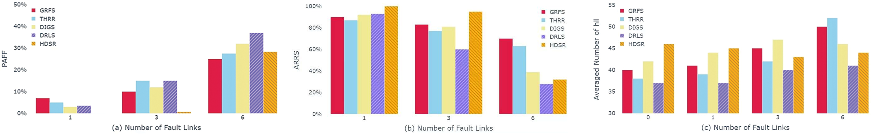
Figure 6: Averaged changes of PAFF, ARRS and hll with the number of fault links

HDSR relies on the fault-tolerance method of redundant paths, and the number of faulty flows is very small when 3 links fail, but when 6 links fail, due to multi-point failures, at least one pair of ENs among the 5 ENs have the redundant paths calculated interrupted, and the number of faulty flows and PAFF increase significantly. THRR and GRFS, due to considering load balance, lead to a certain number of faulty flows with random link failures but have a lower PAFF due to a larger average number of successfully scheduled flows. DIGS and DRLS have link loads mainly concentrated on the shortest path. So when the number of faulty links increases, the probability of link failures on the corresponding shortest path increases, and once a failure occurs, it leads to a larger average number of faulty flows, so there is a higher PAFF.

After the link failure occurs, each strategy reschedules the faulty flows, and the average rerouting and rescheduling success rate of the faulty flows (ARRS) is shown in the Fig. 6b.

Among them, DIGS, because the GCN used is greatly affected by the network topology, only modifies the node link state without changing the existing network topology, while DRLS will calculate a new shortest path according to the updated network and then reschedule. Because HDSR has a higher scheduling cost, the ARRS of HDSR is obviously lower. DRLS, due to poor perception of the graph structure of the network, also has a lower ARRS when facing the network after topological changes. DIGS, although the scheduling performance is too much reduced due to the Laplacian matrix modification without network topology change, aggregated the abnormal features at the time slot of convolution, leading to a significant decrease in its scheduling success rate. THRR’s fault-tolerant method for rerouting and rescheduling of faulty flows performs well in multi-point failures and has achieved a higher ARRS by using the concept of TSN subgraphs and the heuristic weighted KSP algorithm based on traffic priority. However, the PER-MD3QN algorithm used by GRFS has a stronger adaptability to changes in network topology, can perceive the difference between abnormal links and normal links through GAT. So GRFS adapts well to TSN in the fault state, and adjusts the injection time slot offset to make better use of network resources at different time slots, and has the highest ARRS.

As shown in the Fig. 6c, with the increase of faulty links, the hllt of each strategy changes accordingly. GRFS and THRR maintain a high ARRS, so the hllt shows an upward trend.

Among them, GRFS relies on GAT to perceive the changes in resource status of each node, which can flexibly schedule traffic under fault conditions, and improves ARRS while balancing the network resource load as much as possible. Therefore, when there are 6 link faults, GRFS has a smaller hllt compared to THRR, which uses TSN subgraphs to isolate the areas of multi-point faults. DRLS has fewer interrupted flows successfully rescheduled when there are many faulty links, resulting in a smaller increase in hllt. DIGS has a high ARRS when there are 3 link faults and considers less load balancing, so it has a higher hllt, but when there are 6 link faults, the scheduling performance of DIGS is affected, which leads to a decrease in hllt. HDSR shows a downward trend in hllt before multi-point faults cause redundant paths to fail, and due to the high cost of routing and scheduling, the rise in hllt is smaller.

6.2.4 The Impact of MGB Layer Depth on Scheduling Performance

From the above experimental analysis, it is known that GRFS relies on an encoding model based on the GAT residual network to perceive the status of network nodes to achieve flexible traffic routing and scheduling. The depth of the MGB layers will affect the feature extraction capability of the encoding model. Therefore, to further explore the impact of the number of MGB layers on the performance of the algorithm, this section will investigate the performance of GRFS with different numbers of MGB layers in Experiments 1, 2, 3 and 4.

As shown in the Fig. 7a, in Experiment 1, the number of faulty flows in GRFS first decreases with the increase of the number of MGB layers, reaching the best effect when the number of MGB layers is 2, and then increases with the increase of the number of MGB layers. And in Experiments 2, 3 and 4, success rate is always highest when the number of MGB layers is 2 and decreases with the change of the number of MGB layers.

Figure 7: Averaged changes of success rate, hll and time cost with the number of fault links under different MGBs

This is possibly because insufficient training, even though residual connections are added to the MGB, they cannot eliminate the over-smoothing problem. When the number of MGB layers increases, the information propagation in multi-layer GAT will cause the representations of nodes to tend to gather, reducing the distinguishability between nodes, thereby affecting the performance of the model.

The Fig. 7b shows the utilization rate of network resources by GRFS with different numbers of MGB layers, where the scheduling success rate of GRFS is lower and the hllt is similar when the number of MGB layers is greater than 2.

This is because the over-smoothing problem affects the scheduling performance, causing GRFS not to choose the appropriate links when scheduling traffic, so the traffic distribution has a longer transmission path, occupying unnecessary network resources, or the allocated link load is too high.

Moreover, as the number of MGB layers increases, the complexity of the neural network increases, and the response time of PER-MD3QN becomes larger, which may not be able to reroute and reschedule in time when the scale of faulty traffic is large as shown in Fig. 7c.

6.2.5 The Impact of Number of Attention Heads in GAT on Scheduling Performance

To further explore the impact of the number of Attention heads in GAT on the performance of the algorithm, this section will investigate the performance of GRFS with 2 MGB layers and different attention heads in Experiments 1, 2, 3 and 4.

As shown in the Fig. 8a, when the number of attention heads in GAT exceeds 3, an increase paradoxically reduces success rates. The addition of attention heads up to 3 enhances the model’s capacity to represent complex graph structures. However, beyond this, the complexity of the current environment is insufficient for more heads, leading to an information overload that may neglect or weaken key features or relationships.

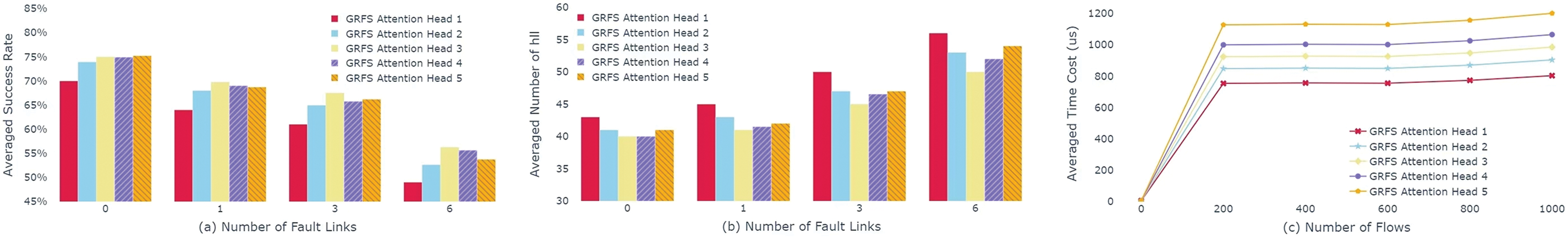
Figure 8: Averaged changes of success rate, hll and time cost with the number of fault links under different attention heads

In Fig. 8b, the minimum of hllt is achieved with 3 attention heads, suggesting excess heads diminish each’s effectiveness, impacting GRFS performance.

However, Fig. 8c shows the increase in heads does not significantly add computational time due to parallel processing.

7  Conclusion and Future Work

In the context of power data communication networks, existing TSN traffic routing and scheduling mechanisms lack fault-tolerance that does not overly affect the scheduling performance under ideal states and can handle permanent faults such as link interruptions. This paper proposes a TS traffic routing and scheduling mechanism based on the fault-tolerant graph attention residual network, GRFS. Unlike most fault-tolerant mechanisms based on TAS and spatial redundancy, GRFS proposes a fusion terminal communication system architecture based on CQF and fault recovery to adapt to the fault-tolerant requirements of the TSN fault state; GRFS constructs an optimized model for joint routing and scheduling that considers traffic delay constraints and network resource constraints and designs a PER-MD3QN algorithm based on the multi-head graph attention residual network to reconstruct the features of TSN and traffic, capturing the changes in the network state of TSN, to solve the joint routing and scheduling problem model. While improving the scheduling success rate, GRFS also aims to balance the network load as much as possible, thereby reducing the number of high-load links and increasing the schedulable traffic volume. By GAT structure optimization and fault tolerance considerations, GRFS expands the use scenarios of GAT in TSN. But GRFS overlooks the temporary faults caused by bit flips. And the processing time of PER-MD3QN used by GRFS does not surpass that of heuristic algorithms when networks and traffic are small scale. Due to the relatively large jitter of CQF and the fact that fault recovery requires a certain amount of time for rerouting and rescheduling, system architecture can only be applied in scenarios that do not emphasize seamless redundancy [28]. The next step is to study how to organically combine time slot redundancy methods to optimize the scheduling mechanism for handling temporary faults, how to minimize fault processing time, or how to combine with spatial redundancy path protection, and provide different protection according to the service level as needed.

Acknowledgement: The authors would like to express appreciation to State Grid Corporation of China Headquarters Management Science and Technology Project Funding for financial support.

Funding Statement: This research was supported by Research and Application of Edge IoT Technology for Distributed New Energy Consumption in Distribution Areas, Project Number (5108-202218280A-2-394-XG).

Author Contributions: The authors confirm contribution to the paper as follows: study conception and design: Zhihong Lin, Zeng Zeng, Yituan Yu, Yinlin Ren, Xuesong Qiu; data collection: Zhihong Lin, Zeng Zeng, Yituan Yu, Yinlin Ren; analysis and interpretation of results: Zhihong Lin, Zeng Zeng, Yituan Yu, Yinlin Ren, Xuesong Qiu; draft manuscript preparation: Zhihong Lin, Zeng Zeng, Yituan Yu, Yinlin Ren, Xuesong Qiu, Jinqian Chen. All authors reviewed the results and approved the final version of the manuscript.

Availability of Data and Materials: Due to the nature of this research, participants of this study did not agree for their data to be shared publicly, so supporting data is not available.

Ethics Approval: Not applicable.

Conflicts of Interest: The authors declare that they have no conflicts of interest to report regarding the present study.

References

1. C. Zhuang, Y. Tian, X. Gong, X. Que, and W. Wang, “A survey of key protocols and application scenarios of time-sensitive networking,” (in Chinese), Telecommun. Sci., vol. 35, no. 10, pp. 31–42, 2019. [Google Scholar]

2. V. Balasubramanian, M. Aloqaily, and M. Reisslein, “Fed-TSN: Joint failure probability-based federated learning for fault-tolerant time-sensitive networks,” IEEE Trans. Netw. Serv. Manag., vol. 20, no. 2, pp. 1470–1486, 2023. doi: 10.1109/TNSM.2023.3273396. [Google Scholar] [CrossRef]

3. M. Pahlevan, S. Amin, and R. Obermaisser, “Fault tolerant list scheduler for time-triggered communication in time-sensitive networks,” J. Commun., vol. 16, no. 7, pp. 250–258, 2021. doi: 10.12720/jcm.16.7.250-258. [Google Scholar] [CrossRef]

4. A. A. Syed, S. Ayaz, T. Leinmüller, and M. Chandra, “Fault-tolerant dynamic scheduling and routing for TSN based in-vehicle networks,” in Proc. IEEE Vehicular Netw. Conf. (VNC), Ulm, Germany, Nov. 2021, pp. 72–75. [Google Scholar]

5. R. Dobrin, N. Desai, and S. Punnekkat, “On fault-tolerant scheduling of time sensitive networks,” in Proc. 4th Int. Workshop on Security and Dependability of Critical Embedded Real-Time Syst. (CERTS 2019), Schloss Dagstuhl-Leibniz-Zentrum fuer Informatik, 2019. [Google Scholar]

6. Y. Zhou, S. Samii, P. Eles, and Z. Peng, “Reliability-aware scheduling and routing for messages in time-sensitive networking,” ACM Trans. on Embedded Comput. Syst. (TECS), vol. 20, no. 5, pp. 1–24, 2021. doi: 10.1145/3458768. [Google Scholar] [CrossRef]

7. Y. Zhou, S. Samii, P. Eles, and Z. Peng, “ASIL-decomposition based routing and scheduling in safety-critical time-sensitive networking,” in Proc. IEEE 27th Real-Time and Embedded Technol. and Appl. Symp. (RTAS), Nashville, TN, USA, May 2021, pp. 184–195. [Google Scholar]

8. C. Chen and Z. Li, “Meta-heuristic-based multipath joint routing and scheduling of time-triggered traffic for time-sensitive networking in IIoT,” in Proc. 2nd Int. Conf. on Green Commun., Netw., and Internet of Things (CNIoT 2022), Xiangtan, China, 2023, vol. 12586, pp. 1–6. [Google Scholar]

9. A. A. Atallah, G. B. Hamad, and O. A. Mohamed, “Routing and scheduling of time-triggered traffic in time-sensitive networks,” IEEE Trans. Ind. Inform., vol. 16, no. 7, pp. 4525–4534, 2019. doi: 10.1109/TII.2019.2950887. [Google Scholar] [CrossRef]

10. H. Chen, M. Liu, J. Huang, Z. Zheng, W. Huang and Y. Xiao, “A heuristic-based dynamic scheduling and routing method for industrial TSN networks,” in Proc. IEEE 10th Int. Conf. on Cyber Security and Cloud Comput. (CSCloud)/IEEE 9th Int. Conf. on Edge Comput. and Scalable Cloud (EdgeCom), Xiangtan, China, Jul. 2023, pp. 440–445. [Google Scholar]

11. Z. Feng, Z. Gu, H. Yu, Q. Deng, and L. Niu, “Online rerouting and rescheduling of time-triggered flows for fault tolerance in time-sensitive networking,” IEEE Trans. Comput. Aided Des. Integr. Circuits Syst., vol. 41, no. 11, pp. 4253–4264, 2022. doi: 10.1109/TCAD.2022.3197523. [Google Scholar] [CrossRef]

12. F. M. Pozo Pérez, G. Rodriguez-Navas, and H. Hansson, “Self-Healing protocol: Repairing scheduels online after link failures in time-triggered networks,” in Proc. 51st IEEE/IFIP Int. Conf. on Dependable Syst. and Netw. (DSN), Taipei, Taiwan, Jun. 21–24, 2021, pp. 129–140. [Google Scholar]

13. W. Kong, M. Nabi, and K. Goossens, “Run-time recovery and failure analysis of time-triggered traffic in time sensitive networks,” IEEE Access, vol. 9, pp. 91710–91722, 2021. doi: 10.1109/ACCESS.2021.3092572. [Google Scholar] [CrossRef]

14. G. Nandha Kumar, K. Katsalis, P. Papadimitriou, P. Pop, and G. Carle, “SRv6-based time-sensitive networks (TSN) with low-overhead rerouting,” Int. J. Netw. Manag., vol. 33, no. 4, 2023, Art. no. e2215. [Google Scholar]

15. A. Kostrzewa and R. Ernst, “Achieving safety and performance with reconfiguration protocol for ethernet TSN in automotive systems,” J. Syst. Archit., vol. 118, 2021, Art. no. 102208. doi: 10.1016/j.sysarc.2021.102208. [Google Scholar] [CrossRef]

16. X. Wang, H. Yao, T. Mai, Z. Xiong, F. Wang and Y. Liu, “Joint routing and scheduling with cyclic queuing and forwarding for time-sensitive networks,” IEEE Trans. Vehicular Technol., vol. 72, no. 3, pp. 3793–3804, Mar. 2023. doi: 10.1109/TVT.2022.3216958. [Google Scholar] [CrossRef]

17. S. Yang, Y. Zhang, T. Lu, and Z. Chen, “CQF-based joint routing and scheduling algorithm in time-sensitive networks,” in 2024 IEEE 7th Adv. Inf. Technol., Electron. and Automat. Control Conf. (IAEAC), Chongqing, China, 2024, pp. 86–91. doi: 10.1109/IAEAC59436.2024.10503933. [Google Scholar] [CrossRef]

18. D. Yang, K. Gong, W. Zhang, K. Guo, and J. Chen, “enDRTS: Deep reinforcement learning based deterministic scheduling for chain flows in TSN,” in Proc. Int. Conf. on Netw. and Netw. Appl. (NaNA), Qingdao, China, Aug. 2023, pp. 239–244. [Google Scholar]

19. X. Wang, H. Yao, T. Mai, T. Nie, L. Zhu and Y. Liu, “Deep reinforcement learning aided no-wait flow scheduling in time-sensitive networks,” in Proc. IEEE Wireless Commun. and Netw. Conf. (WCNC), Austin, TX, USA, Apr. 2022, pp. 812–817. [Google Scholar]

20. L. Yang, Y. Wei, F. R. Yu, and Z. Han, “Joint routing and scheduling optimization in time-sensitive networks using graph-convolutional-network-based deep reinforcement learning,” IEEE Internet Things J., vol. 9, no. 23, pp. 23981–23994, 2022. doi: 10.1109/JIOT.2022.3188826. [Google Scholar] [CrossRef]

21. Y. Huang, S. Wang, X. Zhang, T. Huang, and Y. Liu, “Flexible cyclic queuing and forwarding for time-sensitive software-defined networks,” IEEE Trans. Netw. Serv. Manag., vol. 20, no. 1, pp. 533–546, 2022. doi: 10.1109/TNSM.2022.3198171. [Google Scholar] [CrossRef]

22. J. Yan, W. Quan, X. Jiang, and Z. Sun, “Injection time planning: Making CQF practical in time-sensitive networking,” in Proc. IEEE INFOCOM, Toronto, ON, Canada, Jul. 2020, pp. 616–625. [Google Scholar]

23. W. Quan, J. Yan, X. Jiang, and Z. Sun, “On-line traffic scheduling optimization in IEEE 802.1 Qch based time-sensitive networks,” in Proc. IEEE 22nd Int. Conf. on High Performance Comput. and Commun.; IEEE 18th Int. Conf. on Smart City; IEEE 6th Int. Conf. on Data Sci. and Syst. (HPCC/SmartCity/DSS), Yanuca Island, Cuvu, Fiji, Dec. 2020, pp. 369–376. [Google Scholar]

24. Z. Feng, M. Cai, and Q. Deng, “An efficient pro-active fault-tolerance scheduling of IEEE 802.1Qbv time-sensitive network,” IEEE Internet Things J., vol. 9, no. 16, pp. 14501–14510, Aug. 15, 2022. doi: 10.1109/JIOT.2021.3118002. [Google Scholar] [CrossRef]

25. W. Ma, X. Xiao, G. Xie, N. Guan, Y. Jiang and W. Chang, “Fault tolerance in time-sensitive networking with mixed-critical traffic,” in Proc. 60th ACM/IEEE Design Automat. Conf. (DAC), San Francisco, CA, USA, 2023, pp. 1–6. doi: 10.1109/DAC56929.2023.10247817. [Google Scholar] [CrossRef]

26. J. Cao, W. Feng, N. Ge, and J. Lu, “Delay characterization of mobile-edge computing for 6G time-sensitive services,” IEEE Internet Things J., vol. 8, no. 5, pp. 3758–3773, 2020. doi: 10.1109/JIOT.2020.3023933. [Google Scholar] [CrossRef]

27. S. F. Bush, “Toward efficient time-sensitive network scheduling,” IEEE Trans. Aerosp. Electron. Syst., vol. 58, no. 3, pp. 1830–1842, 2022. doi: 10.1109/TAES.2021.3127311. [Google Scholar] [CrossRef]

28. S. Kehrer, O. Kleineberg, and D. Heffernan, “A comparison of fault-tolerance concepts for IEEE 802.1 time sensitive networks (TSN),” in Proc. IEEE Emerg. Technol. and Factory Automat. (ETFA), Barcelona, Spain, 2014, pp. 1–8. doi: 10.1109/ETFA.2014.7005200. [Google Scholar] [CrossRef]

29. C. Zhong, H. Jia, H. Wan, and X. Zhao, “DRLS: A deep reinforcement learning based scheduler for time-triggered ethernet,” in Proc. Int. Conf. on Comput. Commun. and Netw. (ICCCN), Athens, Greece, IEEE, 2021, pp. 1–11. [Google Scholar]

30. H. Yu, T. Taleb, and J. Zhang, “Deep reinforcement learning based deterministic routing and scheduling for mixed-criticality flows,” IEEE Trans. Ind. Inform., vol. 19, no. 8, pp. 8806–8816, 2022. doi: 10.1109/TII.2022.3222314. [Google Scholar] [CrossRef]

31. Z. Wu, S. Pan, F. Chen, G. Long, C. Zhang and P. S. Yu, “A comprehensive survey on graph neural networks,” IEEE Trans. Neural Netw. Learn. Syst., vol. 32, no. 1, pp. 4–24, Jan. 2021. doi: 10.1109/TNNLS.2020.2978386. [Google Scholar] [CrossRef]

32. J. Zhang, Y. Guo, J. Wang, and Y. Wang, “Enhanced graph neural network framework based on feature and structural information,” (in Chinese), Appl. Res. of Comput./Jisuanji Yingyong Yanjiu, vol. 39, no. 3, pp. 668–674, 2022. [Google Scholar]

33. Q. Xing, Z. Chen, T. Zhang, X. Li, and K. Sun, “Real-time optimal scheduling for active distribution networks: A graph reinforcement learning method,” Int. J. Electr. Power & Energy Syst., vol. 145, 2023, Art. no. 108637. doi: 10.1016/j.ijepes.2022.108637. [Google Scholar] [CrossRef]

34. S. Guo, Y. Lin, N. Feng, C. Song, and H. Wang, “Attention based spatial-temporal graph convolutional networks for traffic flow forecasting,” in Proc. AAAI Conf. on Artif. Intell., Honolulu, HI, USA, 2019, pp. 922–929. [Google Scholar]

35. Z. Cheng, D. Yang, W. Zhang, J. Ren, H. Wang and H. Zhang, “DeepCQF: Making CQF scheduling more intelligent and practicable,” in Proc. IEEE Int. Conf. on Commun. (ICC), Seoul, Republic of Korea, 2022, pp. 1–6. [Google Scholar]

36. D. Yang, Z. Cheng, W. Zhang, H. Zhang, and X. Shen, “Burst-aware time-triggered flow scheduling with enhanced multi-CQF in time-sensitive networks,” IEEE/ACM Trans. on Netw., vol. 31, no. 6, pp. 2809–2824, Dec. 2023. doi: 10.1109/TNET.2023.3264583. [Google Scholar] [CrossRef]

37. Z. Cheng, D. Yang, R. Guo, and W. Zhang, “Joint time-frequency resource scheduling over CQF-based TSN-5G system,” in Proc. 15th Int. Conf. on Commun. Softw. and Netw. (ICCSN), Shenyang, China, 2023, pp. 60–65. doi: 10.1109/ICCSN57992.2023.10297405. [Google Scholar] [CrossRef]

38. X. Wang, H. Yao, T. Mai, S. Guo, and Y. Liu, “Reinforcement learning-based particle swarm optimization for End-to-End traffic scheduling in TSN-5G networks,” IEEE/ACM Trans. on Netw., vol. 31, no. 6, pp. 3254–3268, Dec. 2023. doi: 10.1109/TNET.2023.3276363. [Google Scholar] [CrossRef]