A Discrete Multi-Objective Squirrel Search Algorithm for Energy-Efficient Distributed Heterogeneous Permutation Flowshop with Variable Processing Speed

1  Introduction

The permutation flow-shop scheduling problem (PFSP) is a typical scheduling problem with a wide range of applications, commonly used in large-scale production. In 1954, Johnson first proposed a PFSP scheduling problem [1]. The core idea of PFSP is to divide the production process into multiple stages and allocate each stage to specifically designed production lines, aiming to optimize production efficiency. The work tasks for each production line are specially designed and optimized. Upon completing a stage, a production line transfers materials or products to the next line and proceeds with the subsequent task. Therefore, PFSP can significantly improve production efficiency. Nonetheless, the problem has been proven to be NP-hard when the number of machines exceeds three [2]. Therefore, designing effective algorithms for PFSP holds important academic value and practical significance [3].

On the one hand, the quantity of orders for enterprises has significantly expanded due to the advancement of industrial technology and worldwide trade. Increasingly, managers are recognizing the challenges faced by traditional single factories in meeting market and customer demands within a dynamic production environment [4]. Distributed scheduling, enabling collaborative production among multiple factories, has garnered significant attention for its high production efficiency and optimal resource utilization [5]. Naderi et al. [6] first proposed the distributed permutation flow-shop scheduling problem (DPFSP) in 2010. DPFSP is an extension of PFSP that involves job assignment to factories and the determination of job processing sequences within each factory, rendering it more intricate than PFSP. Gao et al. [7] improved GA and designed effective crossover and mutation operators for DPFSP. Gao et al. [8] also improved TS and proposed a method to generate neighborhood by exchanging working subsequences, which improved the performance of the algorithm for DPFSP. In 2016, Rifai et al. [9] proposed multi-objective DPFSP, taking makespan, total cost and average delay as optimization objectives, and designed an adaptive neighborhood search algorithm to solve this problem. Lin et al. [10] proposed Iterated Cocktail Greedy (ICG) algorithm for DFPSP without waiting, which includes destruction mechanism and two self-coordination mechanisms. Shao et al. [11] proposed a distributed estimation algorithm based on Pareto frontiers and created three probability models to solve sequence-related DPFSP. Lu et al. [12] proposed a multi-objective cooperative optimization algorithm based on Pareto Front, which achieved good convergence in solving DPFSP with buffers. Zhao et al. [13] improved the water wave algorithm and designed four local search methods, exhibiting exceptional performance in optimizing blocked DPFSP scenarios. However, a comprehensive review of prior research reveals that the majority of studies have concentrated on homogeneous factories, characterized by identical machines and processing times. However, in actual production, each factory may have different machine types and processing times, which are called heterogeneous factories. When studying the distributed heterogeneous permutation flowshop problem (DHPFSP), it is essential to consider not only job allocation across multiple factories but also the disparities in machines and processing times, thereby augmenting the problem’s complexity. Additionally, the inclusion of machine and processing time heterogeneity brings the production process closer to real-world requirements. Therefore, numerous scholars have designed corresponding algorithms for DHPFSP. Ruiz et al. [14] presented an iterative greedy algorithm with enhanced initialization, showcasing its effectiveness in optimizing the makespan in DHPFSP. Bargaoui et al. [15] devised a highly efficient heuristic initialization method utilizing chemical reaction optimization (CRO) and incorporating greedy and crossover strategies, exhibiting superior performance on the Taillard benchmarks. Li et al. [16] introduced an improved artificial bee colony algorithm (IABC) for the makespan of DHPFSP, which utilized a workload-balanced initialization method and local search. The effectiveness of IABC was tested on famous benchmarks. Lin et al. [17] improved the backtracking search algorithm and designed effective encoding-decoding schemes and heuristic rules, the results show the strong superiority of the algorithm. These methods mentioned above for DHPFSP have shown excellent performance, but they only optimize the objective of makespan.

On the other hand, as the global economy develops and resource consumption exceeds sustainable levels, the issue of global warming is escalating in severity. Environmental organizations and government institutions have begun to advocate energy-efficient and consumption reduction in various manufacturing sectors. Improving environmental sustainability has emerged as a pressing concern [18]. Statistical data reveals that the manufacturing industry comprises roughly 33% of global energy consumption and contributes approximately 38% to carbon emissions [19]. In light of this, the manufacturing industry has started to attach great importance to reducing energy consumption. Hence, when devising production plans, integrating conventional economic indicators like energy efficiency and completion time is of paramount importance, alongside the development of effective energy-efficient measures and technologies. Researchers have undertaken studies on energy-efficient scheduling problems in DHPFSP. In 2017, Wang et al. [20] considered energy consumption for the first time in DPFSP, and proposed Energy-efficient Distributed Permutation Flow Shop Problem, EDPFSP Afterward, Wang et al. [21] suggested a cooperative memetic algorithm that designed knowledge-driven operators based on the properties of non-dominated solutions, which effectively optimized completion time and TEC in DHPFSP. Li et al. [22] improved the NSGA-II algorithm through the introduction of a novel population generation method and the design of operators targeting completion time and energy consumption in DHPFSP. Zhao et al. [23] designed a self-learning Jaya algorithm and proposed an evaluation criterion that combines TEC and makespan. The higher performance of the suggested method was confirmed by experimental data. Fathollahi-Fard et al. [24] established a new multi-objective heuristic algorithm based on the Social Engineering Optimizer and built a mixed-integer linear model. Experimental outcomes verified the efficacy of the suggested algorithm in reducing energy consumption and model efficiency.

However, a comprehensive analysis of previous research reveals that numerous scholars in the field of DHPFSP have neglected the influence of variable processing speeds on scheduling, or assuming constant speeds. That is, in terms of research objects, there are relatively few researches on distributed workshops with energy-saving performance, and the vast majority of researches still aim at minimizing the makespan, which cannot meet the current diverse scheduling requirements. The Distributed Heterogeneous Permutation Flowshop with variable processing speed (DHPFS-VPS) allows products to be processed on multiple production lines and dynamically scheduled based on real-time conditions to improve production efficiency and reduce costs. Some relevant studies have shown that using variable-speed DPFSP algorithms can effectively reduce waiting and queueing times in the manufacturing process [25]. Considering the need for more efficient workshop scheduling solutions in modern industrial production, DHPFS-VPS holds substantial research value, prompting a growing number of scholars to investigate this problem. Huang et al. [26] proposed a bi-roles co-evolution algorithm (BRCE) for DHPFS-VPS, which designed various local search strategies for energy consumption and machine speeds and proposed an effective energy-efficient strategy. Wang et al. [27] proposed an improved multi-objective whale swarm algorithm (MOWSA) for DHPFS-VPS, which aimed to improve energy efficiency without compromising production efficiency and introduced an updated utilization mechanism for completion time and machine speeds. Generally, research on DHPFS-VPS remains relatively limited, and its exploration is still in the early stages compared to scheduling methods employed for single production lines. Although there are still many challenges in practical applications, such as considering logistics and collaboration between production lines, the concept of DHPFS-VPS has been receiving increasing attention and exploration [28]. Consequently, undertaking further in-depth research in this field holds immense significance and presents promising prospects for practical application.

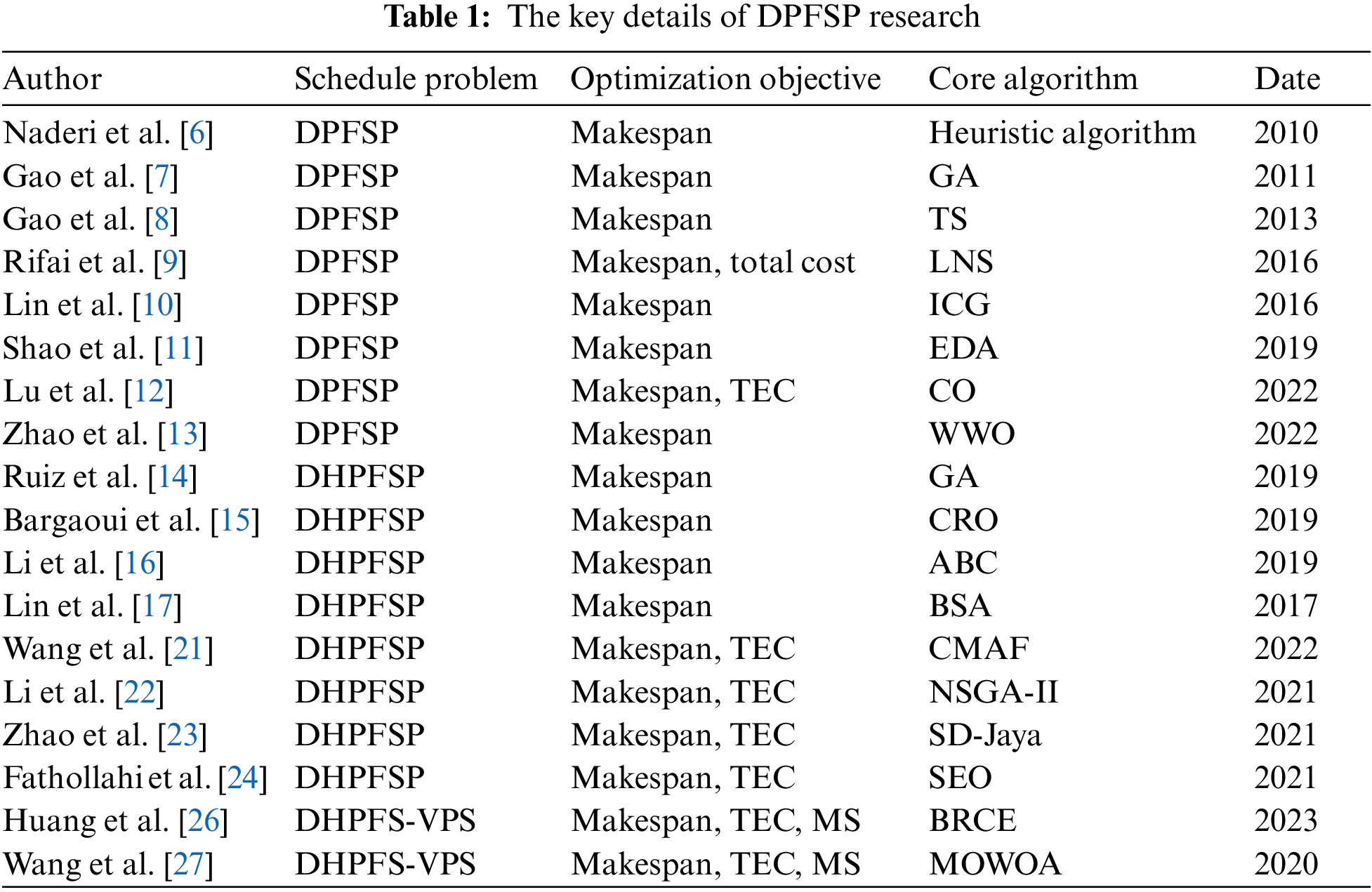
It can be seen that with the deepening of research and the development of industry, the types of DPFSP have gradually become diversified. At the same time, various swarm intelligence algorithms have gradually become the mainstream methods for solving various types of DPFSP. Table 1 summarizes the state of the art of DPFSP research in detail.

The Squirrel Search Algorithm (SSA) is a novel type of swarm intelligence optimization algorithm [29]. Since SSA was proposed, it has been applied to many fields in engineering, including single-objective optimization and multi-objective optimization, demonstrating its practicality and competitiveness in solving engineering problems. It is renowned for its simplistic structure and exceptional performance, making it highly esteemed within the academic community [30]. Currently, there have been multiple studies applying SSA to different fields, such as MEMS vector hydrophone arrays [31], classification of X-ray images [32], and multi-objective economic environmental scheduling. Sakthivel et al. [33] utilized SSA to minimize the total fuel cost and emissions of multi-regional generating units to effectively manage power generation and realize multi-regional economic and environmental scheduling. Wang et al. [34] proposed a dynamic multi-objective SSA and successfully applied it to multi-objective FJSP. Jaishankar et al. [35] used a multi-purpose SSA to secure an efficient blockchain network of healthcare data to generate intelligent and secure healthcare systems, ultimately resulting in 26.87% higher throughput, 34.67% higher efficiency, 22.97% lower latency, 37.03% lower compute overhead, and 34.29% higher storage costs. Guha et al. [36] combined quasi-opposition learning and SSA to develop the controller of wind turbine. Ishwarya et al. [37] combined convolutional neural network and SSA to accurately predict human posture. Maden et al. [38] used SSA to optimize the model parameters of photovoltaic power generation and improve the effectiveness of the photovoltaic system. Nevertheless, research on the discretization of SSA remains limited, and its application to solving the DHPFSP has not been explored. Therefore, this study aims to enrich the application research of SSA and expand the solution methods for DHPFSP-VPS, which holds significant theoretical and practical significance.

The remaining structure of the paper is as follows: In Section 2, the problem is defined, and a multi-objective mixed integer programming model is presented. Section 3 provides an introduction to the standard Squirrel Search Algorithm. In Section 4, the proposed Discrete Multi-objective Squirrel Search Algorithm is described in detail. Section 5 discusses the experimental process and analyzes the results obtained. Finally, Section 6 concludes the paper and suggests potential research extensions for future studies.

2  Problem Description

2.1 Definition of DHPFSP-VPS

DHPFSP-VPS is a highly complex multi-objective combinatorial optimization problem, posing significant challenges to manufacturing production scheduling. The description of DHPFSP-VPS is as follows: There are n(i=1,…,n) jobs and F(f=1,…,F) factories in the problem. Each factory faces a permutation flowshop scheduling problem and is equipped with m(j=1,…,m) machines. Consequently, every job comprises m stages of operations. In the DHPFSP-VPS, the initial step involves assigning each job to a distinct factory. Subsequently, the processing sequence of jobs within each factory needs to be determined. Moreover, the selection of processing speeds for each operation is required. The processing time for each operation of a job is different in different factories, exhibiting heterogeneity. Once a job is assigned to a factory, all its operations are completed within that factory. All jobs start processing on the first machine and finish processing on the last machine. By scheduling the processing sequences within each factory and selecting different processing speeds, distinct makespan, and TEC values can be obtained. Each operation Oij has a standard processing time ti, j on each machine. If the processing speed for Oij is Vv, its actual processing time is Pi, j = ti, j/Vv, and the energy consumption Wi, j is proportional to both Pi, j and Vv2. Therefore, increasing the processing speed leads to a reduction in processing time at the expense of higher power consumption by the machine.

The assumptions of DHPFSP-VPS are as follows:

(1) All machines in all factories are available and ready for processing at time zero, and all factories commence processing at time zero.

(2) Each machine is capable of handling only one operation at a time.

(3) When a job is assigned to a factory, all its operations are carried out exclusively within that factory.

(4) Subsequent operations of a job can only begin once their preceding operations have been completed.

(5) Potential interruptions during job processing and machine failures are not accounted for.

2.2 MILP model for DHPFSP-VPS

To facilitate the description of the model, the notations employed throughout this study are defined as follows:

Indices:

i: set for jobs, i∈{1,...,n};

j: set of machines, j∈{1,...,m};

f: set of factories, f∈{1,...,F};

v: set of speed, v∈{1,...,s};

Parameters:

n: the number of all jobs;

m: the number of machines in each factory;

F: the number of factories;

s: the number of processing speeds;

l: job positions in a sequence, l∈{1,...,n};

Vv: the vth processing speed;

Oi,j: operation of job i on machine j;

Decision variables:

Pi,j: the standard processing time of Oi,j;

Pi,j: the actual processing time of Oi,j;

PPf,j,v: the energy consumption per unit time of machine j in factory f running at speed v;

SPf,j: the energy consumption of the machine j at stand-by mode per unit time in factory f;

PECf,j: processing energy consumption of machine j in factory f;

SECf,j: idle energy consumption of machine j in factory f;

TEC: total energy consumption;

Cmax: the makespan of a schedule;

Cl,j,f: the completion time of position l on machine j in factory f;

C(f): the makespan of factory f;

xi,l,f: a binary variable is defined as 1 when job i occupies position l in factory f, and 0 otherwise.

zi,j,v: a binary variable is defined as 1 when job i process on machine j at speed v, and 0 otherwise

DHPFSP-VPS includes two objectives: makespan and TEC.

The first objective, makespan, is represented by Eq. (1), where the makespan is the sum of the completion times of all jobs.

Makespan=Cmax=maxfC(f)∀f(1)

The second objective, TEC, is represented by Eq. (2), where the energy consumption includes the processing energy consumption (PEC) of all machines in the factories and the idle energy consumption (SEC). The calculation methods for PEC and SEC are demonstrated in Eqs. (3) and (4), respectively.

TEC=∑f=1F∑j=1m(PECf,j+SECf,j)(2)

PECf,j=∑i=1n∑l=1n(xi,l,f⋅pi.j⋅∑v=1szi.j.v⋅ppf,j,v)∀f,j(3)

SECf,j=(C(f)−∑i=1npi,j⋅∑i=1nxi,l,f)⋅SPf,j∀f,j(4)

Makespan and TEC are the two most important indicators in production, and also they are two conflicting objectives. A smaller makespan implies a shorter completion time, which requires higher processing speeds. However, higher processing speeds lead to increased energy consumption. Therefore, to achieve a better balance between the two objectives, it is essential to employ effective scheduling strategies and make appropriate speed selections.

Based on the aforementioned assumptions and the actual production scenario, the constraints of DHPFSP-VPS are as follows:

∑n∑Fxi,l,f=1∀i(5)

∑n∑Fxi,l,f=1∀l(6)

∑v=1szi,j,v=1∀i,j(7)

pi,j=ti,j⋅∑v=1szi,j,vVv∀i,j(8)

Cl,j,f=∑i=1nxi,l,f⋅pi,jl=1,j=1,∀f(9)

Cl,i,f≥Cl,j−1,f+∑i=1nxi,l,f⋅pi,j∀l,j,f(10)

Cl,i,f≥Cl,j−1,f+∑i=1nxi,l,f⋅pi,j∀l>1,j,f(11)

C(f)≥Cl,j,f∀l,f(12)

Cl,j,f≥0∀l,j,f(13)

Cmax=maxfC(f)∀f(14)

xi,l,f∈{0,1}∀i,l,f(15)

zi,j,v∈{0,1}∀i,j,v(16)

Eq. (5) restricts each job to be assigned to a single factory. Eq. (6) guarantees that each machine handles only one job concurrently. Eq. (7) makes sure that each operation is executed at a single speed. Eq. (8) represents the actual processing time for operation Oij. Eq. (9) guarantees that the starting time for the first job on the first machine in factory f is zero. Eq. (10) ensures that each operation of a job can only begin after its preceding operation has finished. Eq. (11) ensures that each machine can only process the next operation after completing the previous one. Eqs. (12) and (13) are processing time constraints for each factory. The makespan objective is defined as Eq. (14). Eqs. (15) and (16) specify the range of binary variables.

2.3 Encoding and Decoding

Encoding method in scheduling occupied an important position in scheduling solution [39]. DHPFSP-VPS, includes three sub-problems: (i) determining the factories for processing each job; (ii) determining the job processing sequence within each factory; (iii) selecting processing speeds for operations. To better utilize DMSSA for solving DHPFSP-VPS, this study adopts a three-stage encoding, which includes job sequence (JS), factory assignment (FS), and variable speed encoding (VS). An example of DHPFSP-VPS with 7 jobs, 2 factories, and 3 speed options is presented in Table 2. In this example, four jobs are processed in Factory 1 with the sequence of 1, 5, 3, 7, while three jobs are processed in Factory 2 with the sequence of 6, 2, 4. Each job consists of three operations, and each factory has three machines dedicated to processing these operations. Assuming a standard processing time of 3 h for each operation, the schedule’s Gantt chart, generated based on the scheduling scheme in Table 2, is depicted in Fig. 1.

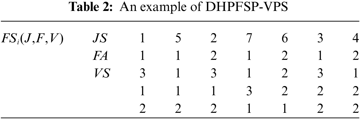
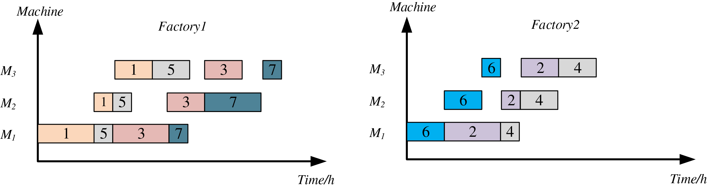
Figure 1: Gantt chart according to Table 2

During the decoding process, jobs are initially assigned to factories based on FA. Subsequently, the job processing sequence within each factory is arranged according to JS. Lastly, the processing speeds for each operation of the jobs are determined based on VS. The actual processing time is calculated by dividing the standard processing time by the processing speed. The processing energy consumption can be calculated based on the principle that it is positively correlated with the square of the processing speed.

3  Squirrel Search Algorithm

3.1 Description of the Squirrel Search Algorithm

Squirrel Search Algorithm (SSA) is a new swarm intelligence algorithm proposed in recent years, which has been proved to be highly competitive in solving real-world problems. However, there is no research on the application of multi-objective squirrel search algorithm in distributed job shop scheduling. SSA is a three-population based algorithm, which has excellent population cooperation ability and can avoid blind crossover and mutation in scheduling optimization, which is very important for complex combinatorial optimization problems. In addition, energy-efficient distributed job-shop scheduling usually involves a large number of job and resource problems, and the data dimension of the optimization problem is high, while the excellent performance of SSA in dealing with similar high-dimensional data makes it may be a suitable choice to deal with such problems. In view of this, as well as the advantages of SSA compared with other algorithms in convergence speed and avoiding local optimum, this paper chooses SSA algorithm to solve the optimal energy-saving distributed job shop scheduling problem.

SSA proposed by Jain et al. [29] in 2018 based on the dynamic feeding and gliding behavior of flying squirrels. Flying squirrels possess a parachute-like membrane that enables them to alter lift and air resistance effortlessly during gliding, exhibiting a complex and energy-efficient aerodynamic motion. During warm seasons, squirrels glide continuously among forest trees in search of food and to store excess provisions. However, in winter, reduced food availability and leaf scarcity increase the risk of predation, resulting in decreased squirrel activity. Squirrels only regain their activity levels at the end of winter. Three assumptions are formulated to enhance the simulation of squirrel behavior:

(1) Each squirrel in the forest occupies a tree individually.

(2) The forest comprises three types of trees: hickory, oak, and normal trees. Hickory trees offer the highest-quality food, oak trees provide regular food, while normal trees do not have any food resources.

(3) The forest consists of a single hickory tree and three oak trees, while the remaining trees are normal trees.

Under the given assumptions, the positions of each squirrel are randomly initialized. Then, the fitness of each squirrel is evaluated, and the individuals are sorted in ascending order based on their fitness. The squirrel with the best fitness is assigned to the hickory tree, and the squirrels ranked 2nd to 4th in terms of fitness are assigned to the oak trees. The remaining squirrels are allocated to the normal trees.

3.2 Individual Location Update Methods

Squirrels update their positions by gliding across different trees. The updating of squirrel positions can be categorized into three stages, determined by the initial and final positions of their glides.

Step 1: Squirrel located on oak tree moves towards the hickory tree using the position update method described by Eq. (17).

FSatt+1={FSatt+dg×Gc×(FShtt−FSatt)R≥Pdprandomlocationotherwise(17)

where FSat is the location of the squirrel on the oak tree and FSht is the location of the squirrel on the hickory tree. dg represents a random gliding distance, Gc is a gliding parameter, and R is a random number in [0,1]. Pdp represents the probability of the presence of a predator.

Step 2: Squirrel located on normal tree migrates to the oak tree using the position update method depicted in Eq. (18):

FSntt+1={FSntt+dg×Gc×(FSatt−FSntt)R≥Pdprandomlocationotherwise(18)

Step 3: Squirrel located on normal tree relocates to the hickory tree using the location update method illustrated in Eq. (19):

FSntt+1={FSntt+dg×Gc×(FShtt−FSntt)R≥Pdprandomlocationotherwise(19)

3.3 Season Detection Condition

To avoid local optima, a seasonality detection condition is introduced after the movement of all individuals. Eq. (20) is used to determine the seasonality constant, and Eq. (21) is used to determine the minimum value:

Sct=∑k=1d(FSat,kt−FSht,k)2t=1,2,3(20)

Smin=10e−6(365)t/(T/2.5)(21)

where T represents the maximum number of iterations, t represents the current iteration. When Sct<Smin, the seasonality condition is satisfied, indicating the end of winter. At this stage, squirrels that have not found food yet are randomly repositioned according to Eq. (22). In the formula, Le´vy(n) is the step size that follows a levy distribution in the random walk model, and FSU and FSL represent the upper and lower bounds of the individual’s position, respectively.

FSntnew=FSL+Le´vy(n)×(FSU−FSL)(22)

4  The DMSSA Is Designed Specifically for the DHPFS-VPS Problem

4.1 Hybrid Initialization Strategies

Employing effective initialization methods can substantially enhance the quality of the initial population, benefiting both the algorithm’s rapid convergence and the final solution’s quality. Hence, designing an effective initialization strategy for DHPFS-VPS holds immense significance. Four hybrid initialization strategies are proposed, each based on distinct optimization objectives, as follows:

(1) The principle of makespan prioritizing: To minimize the maximum completion time of the schedule, the processing speeds of all machines are set to the maximum. Firstly, JS and FA are randomly initialized, and then the VS of all operations is set to the maximum. This step aids in minimizing the makespan.

(2) The principle of TEC prioritizing: To minimize the energy consumption of the schedule, the processing speeds of all machines are set to the minimum. Similarly, JS and FA are randomly initialized first, and then the VS of all operations is set to the minimum. This step aids in reducing energy consumption during processing.

(3) To prevent one factory from processing an excessive number of jobs, which could lead to a longer overall makespan, the factory with the lowest current workload is selected when assigning jobs to factories. Firstly, JS and VS are randomly initialized, and then the processing times of all machines in each factory are evaluated. The factory with the shortest processing time for a job is chosen to generate FA. If multiple factories have an equal workload, one of them is randomly selected.

(4) Random initialization: The diversity of the initial population is crucial for achieving the final scheduling solution [39]. Therefore, as part of this study, a portion of the individuals adopt a random initialization strategy that involves the random initializing of JS, FA, and VS. This step will help enrich the diversity of the population.

To effectively implement the aforementioned four strategies, a quarter of the individuals are generated for each strategy. The adoption of a hybrid initialization strategy allows for a thorough exploration of the extreme spaces of the two objectives and ensures diversity in the initial population. This approach is beneficial for increasing the distribution of solutions and accelerating the convergence speed of the algorithm.

4.2 Improved Strategies for Making DMSSA Applicable to Discrete Scheduling Problems

4.2.1 Improved Population Hierarchy

In the standard SSA, the population is categorized into three categories: one squirrel perched on a hickory tree, three squirrels on oak trees, and the remaining individuals on normal trees. During foraging, collaboration is required. However, the basic SSA exhibits slow convergence speed and premature convergence. This is because the SSA relies only on the guidance of four squirrels, which weakens the information exchange and cooperation among the population, to some extent limiting the algorithm’s search capability. In the process of collective search, having too few guiding individuals weakens the group’s collaborative ability and leads to a linear centralization of population decision-making. This is reflected in the convergence process, where the algorithm cannot escape the domain of local optimal solutions and experiences premature convergence.

This study improves the population hierarchy system of squirrels by adjusting the distribution proportions of the population individuals as follows: 10%: 30%: 60%, as shown in Fig. 2, where “ps” represents the population size. Following the improvement, the number of individuals in categories FSht and FSat increases, enhancing the guiding role of the head individuals. As this research deals with a multi-objective problem, a sorting method akin to the non-dominated sorting and crowding distance employed in the NSGA-II algorithm is utilized to rank the individuals. The top 10% of the sorted individuals are assigned to hickory trees, followed by assigning 10% to 40% of individuals to oak trees and allocating the remaining 60% of individuals to normal trees.

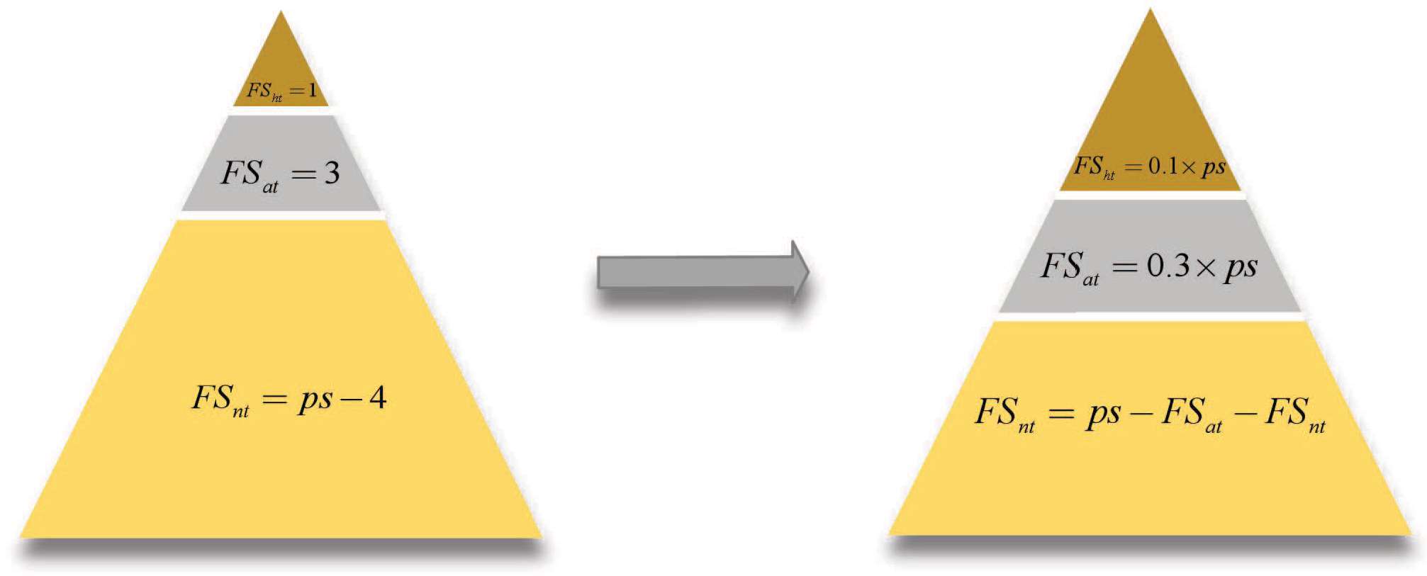
Figure 2: Improvement of the algorithm population hierarchy

4.2.2 Improved Position Updates

DHPFS-VPS is a discrete problem, while SSA is continuous, so it is necessary to improve the position update method. The improved DMSSA categorizes the squirrel movement into three stages, corresponding to the three types:

Step 1: The squirrels on the oak tree (FSat ) move towards the hickory tree (FSht). In the absence of predators (R ≥ Pdp), individuals on the hickory trees guide the individuals on the oak trees using discrete Partial Match Crossover (PMX) for JS. Fig. 3 illustrates an example of PMX. Firstly, squirrels located on the hickory trees and oak trees are selected, respectively. Then, two different points are randomly selected, and the permutations between these two points are exchanged to generate two offspring FS1 and FS2. These generated individuals may contain illegal solutions and require mapping.

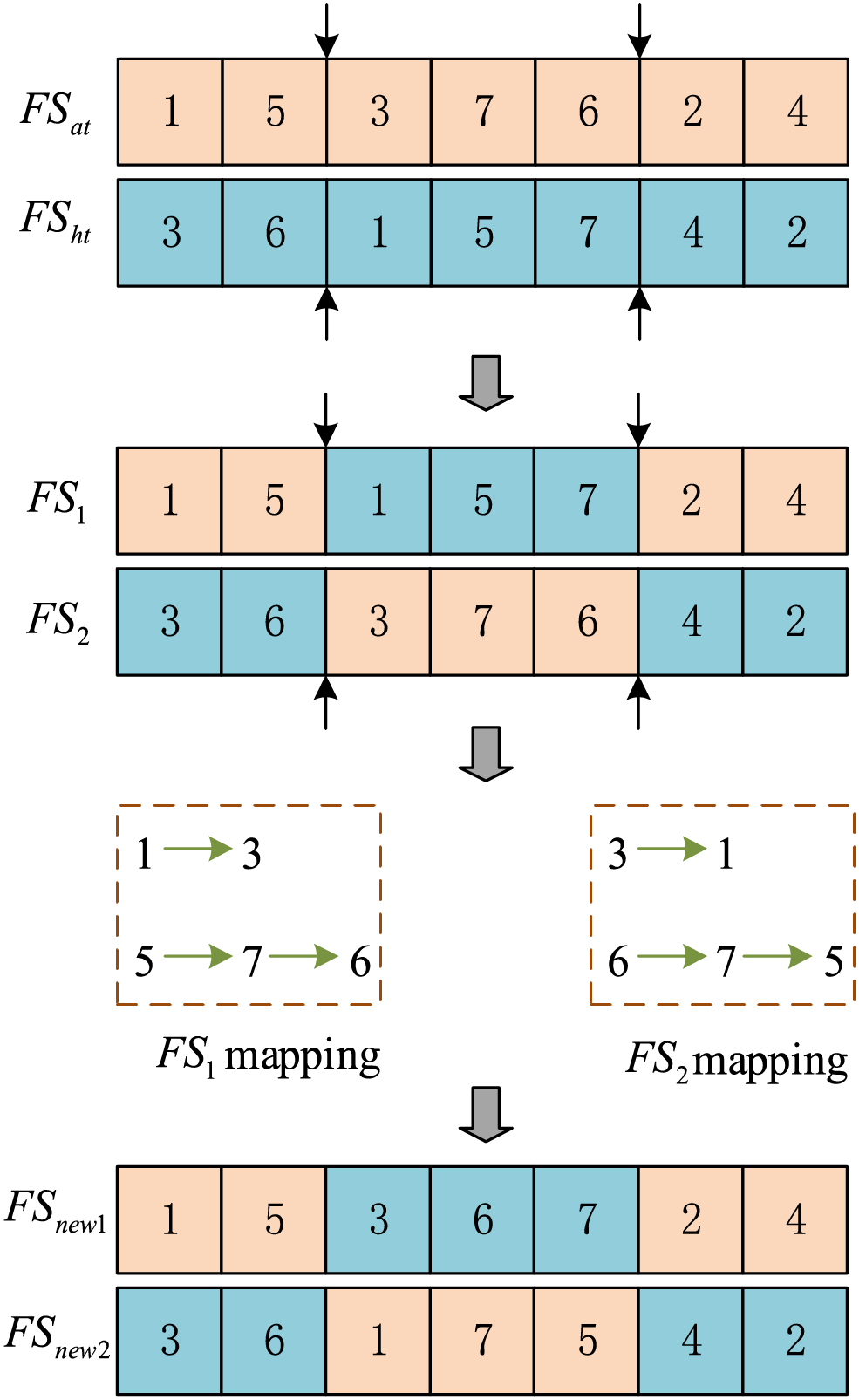
Figure 3: PMX

As shown in Fig. 3, there are repetitions in Jobs 1 and 7 in FS1. Similarly, there are repetitions in Jobs 3 and 6 in FS2. For FS1, the repeated job 1 is replaced with the corresponding Job 3 in FS2. Likewise, Job 5 is replaced with Job 7, and the extra Job 7 is then replaced with Job 6. For FS2, after applying the same replacement operation, the final two new individuals FSnew1 and FSnew2 are generated.

Since there is no correlation between the factory assignment and speed settings of each job, and speed settings do not have permutation constraints, Uniform Crossover (UX) is used for FA and VS. UX randomly selects corresponding encodings of two individuals for exchange. Fig. 4 illustrates a schematic diagram of UX.

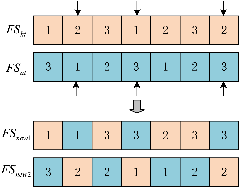
Figure 4: UX

When a predator is present (R < Pdp), the squirrel’s movement is not guided by superior individuals, and in the standard SSA, the squirrel randomly moves to other positions. However, in this case, as FSat is already a better individual, randomly moving to other positions would result in the loss of its previous memory, which is unfavorable for algorithm convergence. Thus, in this paper, the random movement of FSat is improved by importing the local search methods introduced in Section 4.3.1. Local search are conducted near the current position, which not only retains the previous memory but also prevents the algorithm from getting trapped in local optima. The movement of FSat after the improvement of Eq. (17) is shown in Eq. (23), where ⊗ denotes crossover.

FSatt+1={FSatt⊗FShttR≥PdpFSattlocalsearchotherwise(23)

Step 2: The squirrels on the normal tree (FSnt) move towards the hickory tree (FSht). In the absence of natural enemies (R ≥ Pdp), individuals on the hickory trees guide individuals on the normal trees, following a similar approach as described in Eq. (23). For JS, PMX guidance is still used, while UX guidance is employed for FA and VS. When natural enemies are present (R < Pdp), a mutation approach is used instead of the “random location” described in Eq. (18), which is advantageous for increasing the population’s diversity. For JS, the mutation involves randomly swapping the positions of two items. For FA, the mutation entails randomly selecting an item and reassigning it to a different factory. For VS, the mutation entails randomly selecting an operation and changing its speed. The improved movement approach for Eq. (18) is described in Eq. (24).

FSntt+1={FSntt⊗FShttR≥PdpFSnttmutationotherwise(24)

Step 3: The squirrels on the normal tree (FSnt) move towards oak trees (FSat). The movement approach in this step follows the same approach as in Step 2, and the improved movement approach for Eq. (19) is described in Eq. (25).

FSntt+1={FSntt⊗FSattR≥PdpFSnttmutationotherwise(25)

4.3 Search Strategy

4.3.1 Local Search Strategy

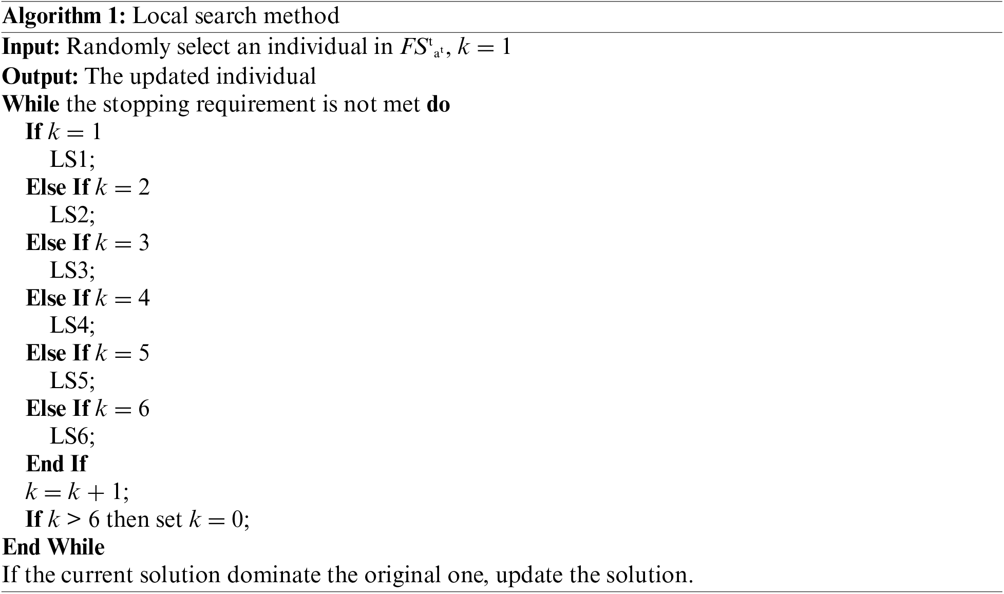
In the standard SSA, the superior individuals on the oak trees may undergo random initialization to other positions, as shown in Eq. (17). This causes the superior individuals to completely abandon their prior memory, resulting in a considerable loss of the previous iterative outcomes. To address this issue, an improvement is proposed in this study. When R < Pdp, a local search strategy is applied to the individuals on the oak trees. Designing an effective local search strategy can greatly enhance the individuals’ search ability and have a positive impact on scheduling outcomes [40]. Therefore, based on the characteristics of DHPFS-VPS, this study introduces the following six local search strategies for the individuals on the oak trees. Each local search algorithm needs to be executed sequentially, ensuring equal triggering frequency for all six algorithms. For detailed implementation, please refer to Algorithm 1.

LS1: Randomly select two jobs and swap their positions, as shown in Fig. 5a. This operation helps increase the diversity of solutions.

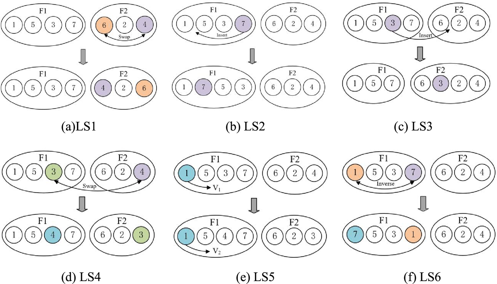
Figure 5: Local search

LS2: Perform an insertion operation within the critical factory. Within a critical factory, randomly select a critical operation and insert it at another possible position in the factory, as shown in Fig. 5b.

LS3: Perform an insertion operation outside the critical factory. Within a critical factory, randomly select a critical operation and insert it into a possible position in another factory, as shown in Fig. 5c. This helps reduce the makespan.

LS4: Exchange operation between factories. Randomly select two factories, then randomly select two operations and exchange their positions, as shown in Fig. 5d.

LS5: Perform a speed increase operation within critical factories. Within a critical factory, randomly select a critical operation and increase its processing speed, as shown in Fig. 5e. This helps reduce the makespan.

LS6: Perform an exchange operation within critical factories. Within a critical factory, randomly select two critical operations and swap their positions, as shown in Fig. 5f.

4.3.2 Dynamic Predator Strategy based on Q-Learning

(1) An introduction to Q-Learning

Watkins et al. [41] first introduced Q-learning in 1992, which has now become one of the most famous reinforcement learning methods. It assists algorithms in selecting optimal parameters throughout the iteration process and enhancing algorithm performance. Q-learning is comprised of a quintuple (A, E, C, S, R), representing the Agent, Environment, Action set, State set, and Reward. Referring to Fig. 6, the Agent performs action At based on its current state St at time t in the Environment, then receives reward Rt+1, and its state transitions to a new state St+1. Eq. (26) is used to update the Q-value as follows:

Q(St,At)=Q(St,At)+α[Rt+γmax(Q(St+1,At)−Q(St,At))](26)

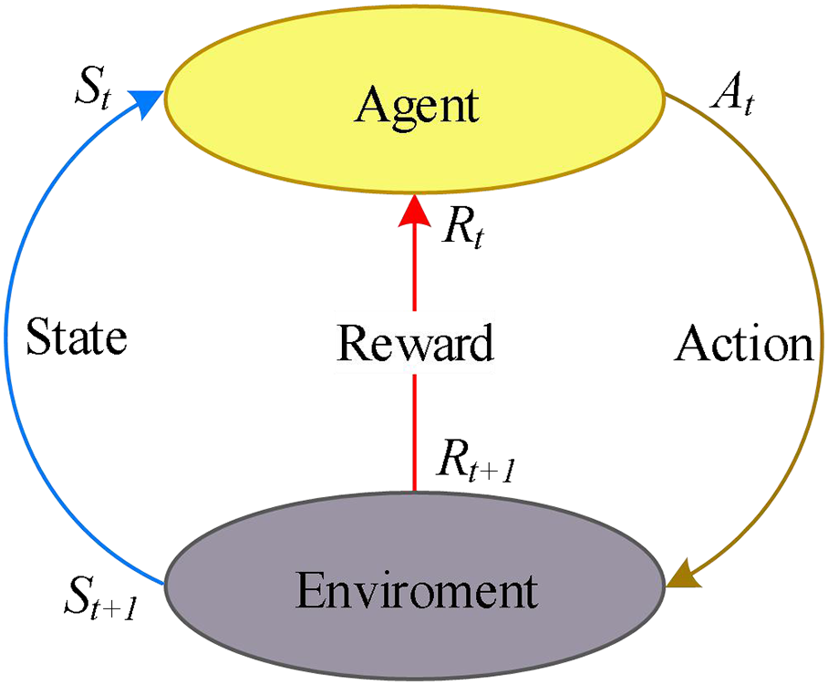
Figure 6: Q-learning

Q(St, At) represents the Q-value when taking action At in state St, Rt represents the reward signal, α is the learning rate, and γ is the discount factor. This formula means that after taking action At, we receive an immediate reward Rt and add it to the maximum Q-value of the next state St+1, updating the corresponding element in the Q-table. This operation is controlled by α, which determines the learning speed, but it is also influenced by γ, which represents the future rewards in the next stage of the Q-value. When α tends to 0, the immediate reward has minimal impact on the current Q-value, leading to slower learning but more stable learning. Conversely, larger values of α enable faster learning but may lead to unstable Q-values.

(2) Definition of agent and action

In SSA, the probability of predator existence, denoted as Pdp, affects the individual’s movement direction. In the standard SSA, Pdp is a fixed value of 0.1, which is obviously not conducive to dynamically selecting the movement mode of the algorithm during iteration [42]. Tooptimize the selection of individual movement directions at different stages of iteration and obtain a better Pareto solution set, a dynamic Pdp based on Q-learning is designed. The predator existence probability for each generation is abstracted as an agent, representing the successful parameter selection. Three candidate values for the predator existence probability are set: Pdp = 0.3, 0.5, and 0.7.

(3) State setting

The changes in the Agent’s state provide feedback to Q-learning to determine whether the action taken can improve the quality of the Pareto Front (PF). To describe the state, convergence (CV) and diversity (DV) metrics are defined, as shown in Eqs. (27) and (28):

CV(P,P∗)=∑y∈Pminx∈P∗dis(x,y)2|P|(27)

DV=∑i=1N−1|di−d−|(N−1)d−(28)

The calculation of CV and DV is similar to LI, etc. [43]. Here, P represents the PF obtained by the algorithm, and P* is a predefined reference point. di denotes the Euclidean distance between adjacent points in the PF, and d− is the average of di values. A smaller CV is better, while a larger DV is better. To describe the changes in the state, Eqs. (29) and (30) provide the calculation methods for the variations of CV and DV at each iteration.

△CV=CVi−1−CVi(29)

△DV=DVi−DVi−1(30)

According to the different values of △CV and △DV during the iteration process, four states are defined, namely:

(1)△CV>0,△DV>0;

(2)△CV>0,△DV≤0;

(3)△CV≤0,△DV>0;

(4)△CV≤0,△DV≤0;

Specifically, (1) and (2) occur in the early stages of iteration, where the population is relatively scattered. (3) and (4) occur in the later stages of iteration, where the population becomes more clustered.

(4) Definition of reward

Following the execution of an action, the agent is either rewarded or punished. The selected action will be rewarded if it increases the PF’s diversity; otherwise, it will be punished. For this study, the maximum reward value is predetermined as 10, as used in previous research. To mitigate the impact of punishment on previous rewards, the punishment is set to 0. The definition of rewards in this paper is shown in Eq. (31):

Reward={10△DV>00△DV≤0(31)

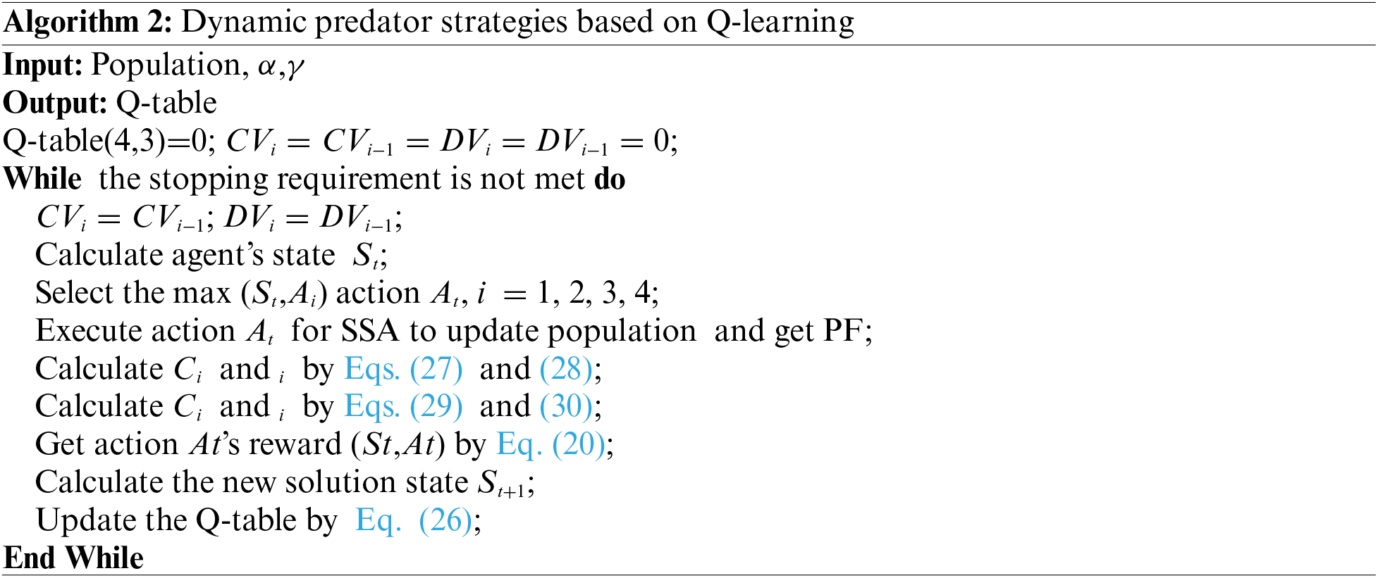
(5) Based on Q-learning parameter selection

Algorithm 2 describes the details of parameter selection based on Q-learning. Firstly, the Q-table is initialized with all zeros, and CV and DV as well as the state St are initialized. Then, the action At is executed, resulting in PF, and ΔCV and ΔDV are updated. The agent transitions to the next state St+1. Lastly, the (St, At) in the Q-table is updated using Eq. (26).

4.4 Speed Control Energy-Efficient Strategy

TEC, an additional crucial objective of DHPFS-VPS. Designing effective energy-efficient techniques is a key technology for energy scheduling. However, in DHPFS-VPS, makespan and TEC are two conflicting sub-objectives, where improving one objective may lead to the deterioration of the other. Based on this characteristic, this paper presents two speed control energy-efficient strategies that specifically address idle time. These strategies can adjust the processing speed of the machine, reducing energy consumption and minimizing idle time with no impact on makespan.

Speed reduction strategy be applicated to when the start time of an operation on the same machine is greater than the end time of the previous operation, idle time is generated. Therefore, reducing the processing speed of the operation before the idle time period can effectively decrease idle time, as shown in Fig. 7. After implementing this operation, the processing speeds of operations O5,2, O5,3, and O3,3 are slowed down, and the idle time T1 and T2 disappear, T3 reducing by half to T’3. The critical path, representing the longest path from the start to the end, determines the makespan of this schedule. To ensure that the makespan is not affected, this operation must be applied solely to non-critical operations outside the critical path.

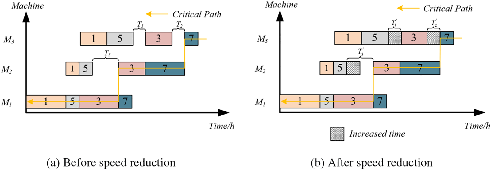
Figure 7: Speed reduction strategy

Speed increase strategy be applied when idle time is generated due to the excessive processing time of a preceding operation, as in Fig. 7a where the operation O3,2 has excessive processing time, causing the start time of O3,2 to be later than the end time of O5,2, a period of idle time is created. Thus, by appropriately increasing the processing speed of O3,1, and reducing its processing time, the start time of O3,2 can be advanced, consequently reducing idle time. As shown in Fig. 8, the implementation of the speed increase strategy not only reduces idle time but also decreases the makespan.

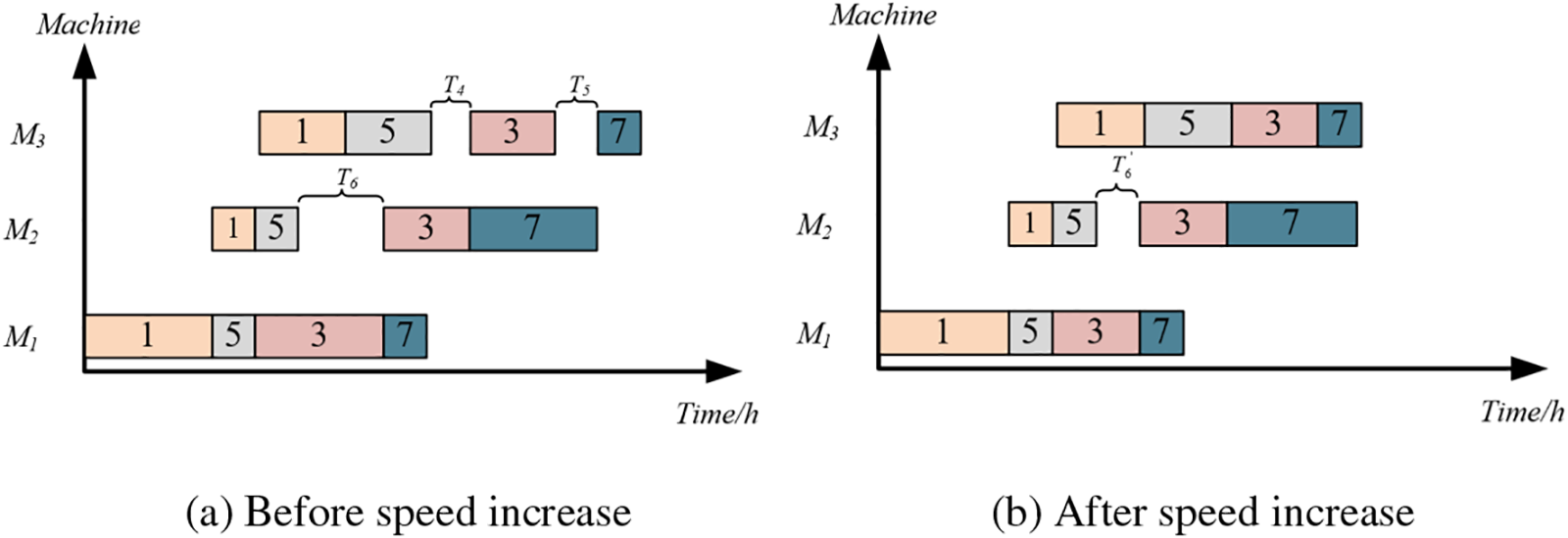
Figure 8: Speed increase strategy

The speed reduction strategy extends the completion time of the preceding operation before idle time, whereas the speed increase strategy advances the start time of the succeeding operation after idle time. Both strategies can reduce energy consumption without increasing the makespan. To balance the number of machines, a random selection probability of 0.5 is set for each of the two strategies. Furthermore, to minimize runtime, we specify that the execution of the strategies should only occur when the working time exceeds 80% of the total time. This strategy serves as a comprehensive alternative to the seasonal detection condition discussed in Section 3.3 of SSA.

4.5 Framework of DMSSA

The overall framework of DMSSA, incorporating the search components mentioned above, including hybrid initialization, local search, population position updates, parameter selection, and energy-efficient strategy, is illustrated in Fig. 9. Firstly, high-quality solutions are generated using hybrid initialization. Secondly, individuals are subjected to a non-dominated sorting based on crowding distance, and positions are allocated to all individuals. Next, the Q-learning is employed to select the optimal Pdp. Subsequently, individual position information is updated using an improved position update approach. Finally, the speed control energy-efficient strategy is applied to effectively reduce TEC.

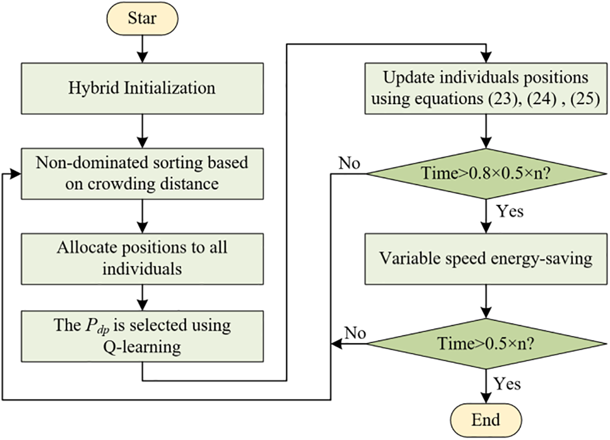
Figure 9: Framework of the DMSSA for DHPFSP-VPS

5  Experimental Results and Discussion

5.1 Performance Metrics

(1) Hypervolume (HV) [44]: HV can evaluate the distribution of Pareto solutions in the objective space. A larger HV value indicates better overall performance of the algorithm. Eq. (32) shows how to calculate it:

HV(P,r)=∪x∈ppv(x,r)a(32)

In the equation, P represents the Pareto solution set obtained by each algorithm, r is the reference point, and let r be (1.1, 1.1). x represents a normalized Pareto solution, and v represents the volume of the hypercube.

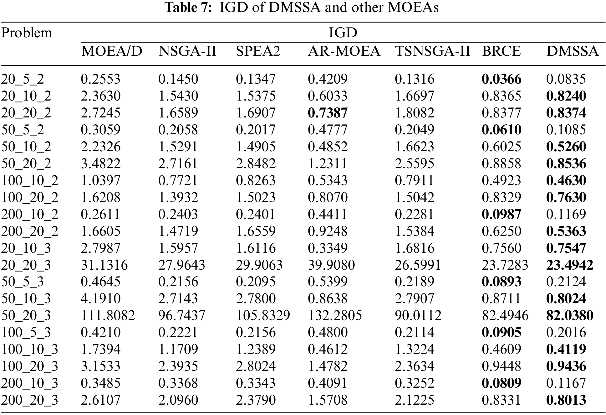
(2) Inverse Generational Distance (IGD) [45]: It primarily evaluates the convergence and distribution of an algorithm. A smaller IGD value indicates better performance. The calculation formula is shown in Eq. (33):

IGD=∑i=1ndi∗2n(33)

In the equation, di represents the Euclidean distance between each point in the true Pareto front (PF*) and the nearest point obtained by the algorithm’s Pareto front. n represents the number of points in PF*. Since the true values of PF* are unknown, in this study, the PF* for each problem is obtained from the runs of all the algorithms.

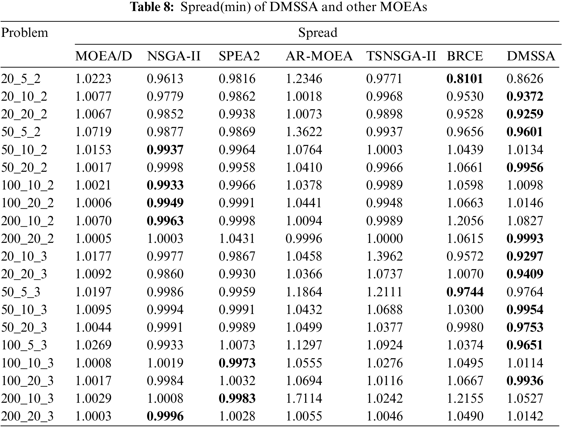
(3) Spread [46]: It measures the diversity of a solution set by quantifying its extent of spread. A smaller Spread value indicates better performance. The mathematical expression is provided in Eq. (34):

Spread=df+dl+∑i=1N−1|di−d−|df+dl+(N−1)d−(34)

In the equation, d represents the distance between extreme solutions on the Pareto approximate solution set, and di represents the distance between boundary solutions of each objective. N is the number of individuals in the approximate solution set. d is the average value of all di distances.

5.2 Test Problem

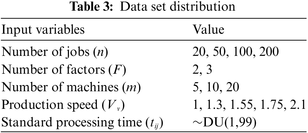
Currently, there is no available open-source benchmark specifically designed for DHPFS-VPS. In this study, Reference [26] served as the basis, and a total of 20 different problems are generated using the Taillard benchmark. These problems are named following the n-m-F notation. The specific parameters are presented in Table 3, where n = {20, 50, 100, 200}, F = {2, 3}, m = {5, 10, 20}, and Vv = {1, 1.3, 1.55, 1.75, 2.1}. Each operation’s standard processing time follows a uniform distribution U(1, 99). In heterogeneous factories, each operation has different processing times in different factories. The processing power is set to 2.0 kWh, with the idle power is set to 1.0 kWh. The CPU stopping time is set to 0.5×n s. All codes are programmed using MATLAB 2019b, and the software is run on a system with an Intel(R) Core(TM) i9-9900K CPU @ 3.60 GHz and 64 GB RAM, operating on a Windows 10 system. Each problem is independently run 20 times to confirm the reliability of the results.

5.3 Parameter Settings

The performance of an algorithm is influenced by multiple factors, with parameters being particularly significant. Therefore, it is crucial to determine the optimal parameters for algorithmic applications. In DMSSA, there are three parameters: the population size (ps), the learning rate (α), and the decay rate (γ). This study adopts the Taguchi method of design of experiment (DOE) [47] to find the optimal parameters by setting parameter levels. Based on mainstream parameter settings, this study sets the parameter levels as follows: ps = 50, 100, 150. γ = 0.7, 0.8, 0.9. α = 0.1, 0.2, 0.3.

A calibration experiment is conducted using an orthogonal array L9(33). Each parameter is independently run 30 times on the 20_5_2 problem, and the average HV are calculated. As shown in Fig. 10, we evaluate the impact of the three parameters on the HV value. Considering the comprehensive influence, the optimal configuration of the parameters is ps = 100, γ = 0.9, α = 0.2.

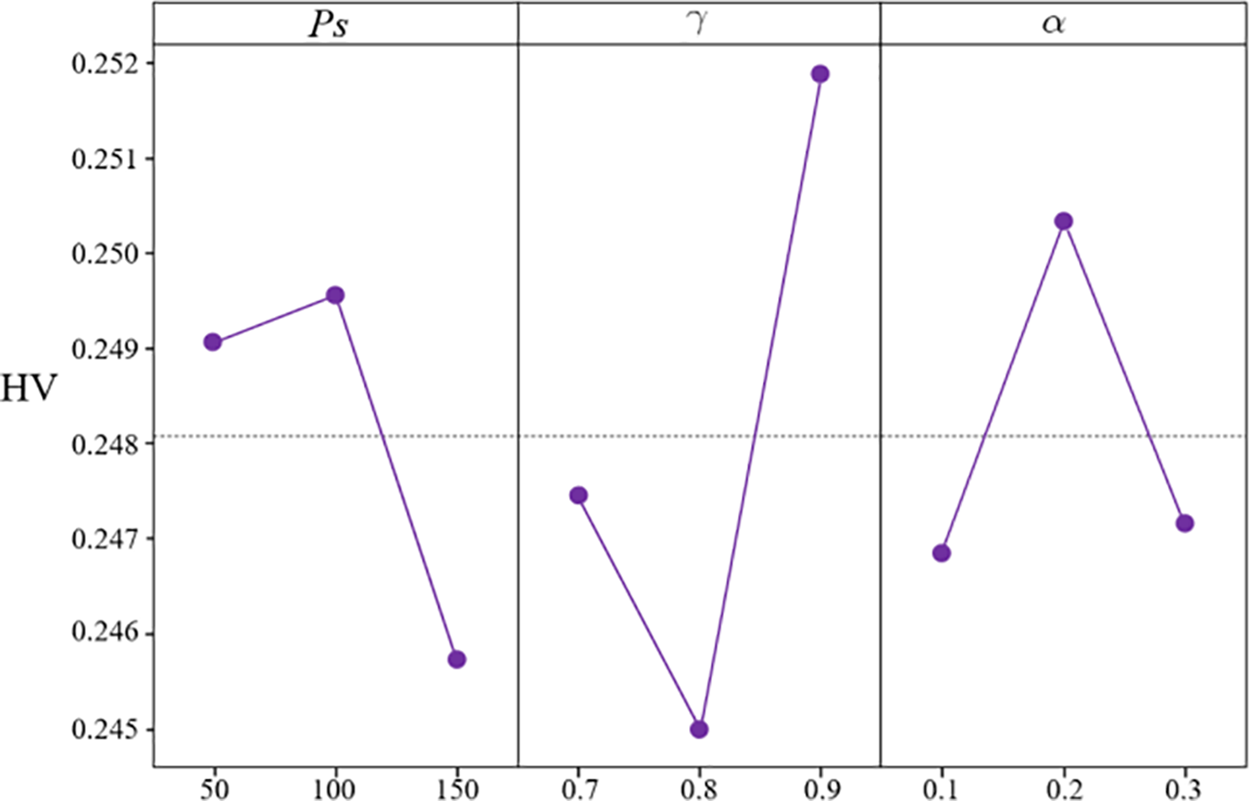
Figure 10: Main effects plot of HV

5.4 Effectiveness of Hybrid Initialization

To demonstrate the competitiveness of the population generated through hybrid initialization, 100 individuals are generated using both hybrid initialization and random initialization on the 20_10_2 problem. Fig. 11 displays the box plots of the individuals generated by both methods for the two objectives. After comparing and analyzing the individuals generated by the two different initialization methods on the two objectives, the results indicate that the population generated by hybrid initialization has higher quality. Specifically, on makespan and TEC, the population generated by hybrid initialization exhibits a broader distribution, enabling better exploration and utilization of the objective space, as seen in Fig. 11a,b. In contrast, the individuals generated by random initialization are relatively concentrated, constraining the population’s evolutionary development space. These results suggest that, in the selection of the initial population, hybrid initialization is a more effective and appropriate strategy.

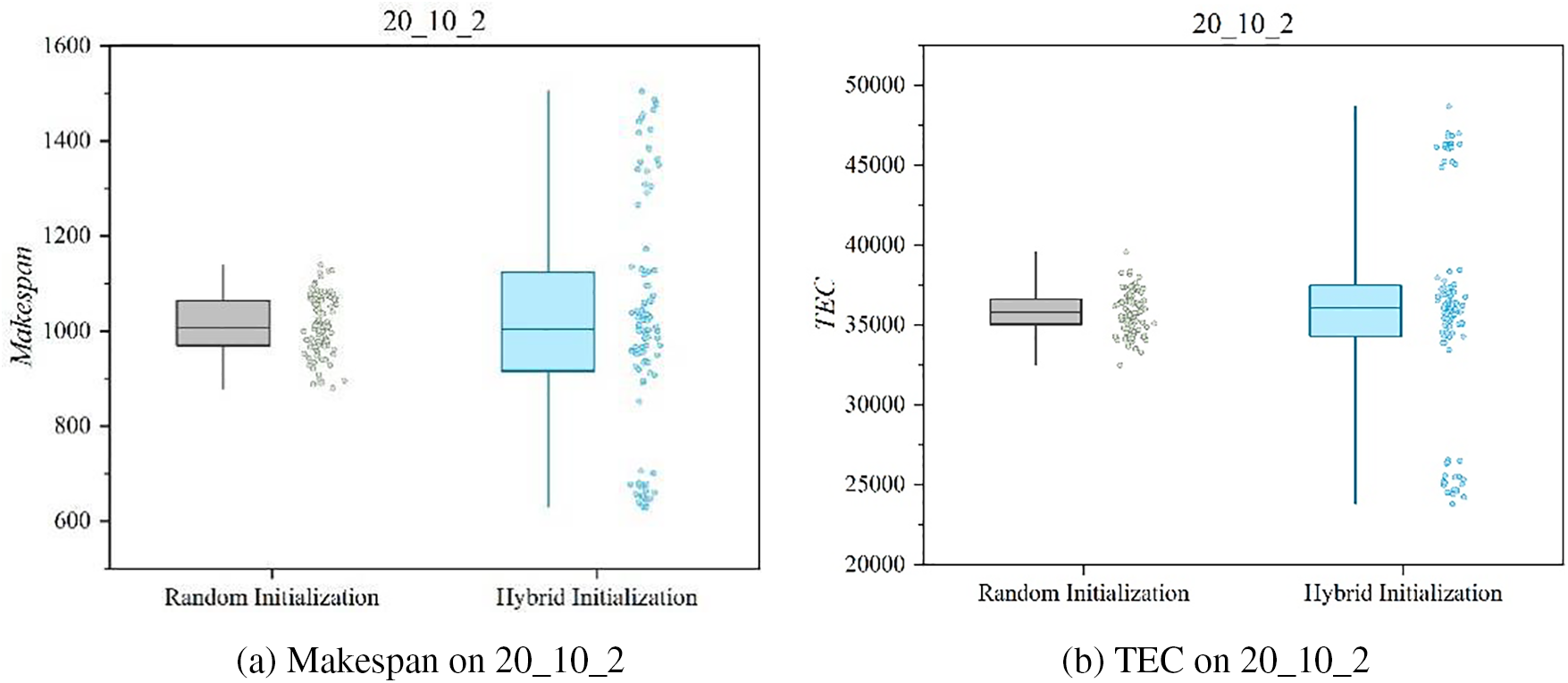
Figure 11: Population boxplot generated by two methods

5.5 Effectiveness of Local Search Strategy

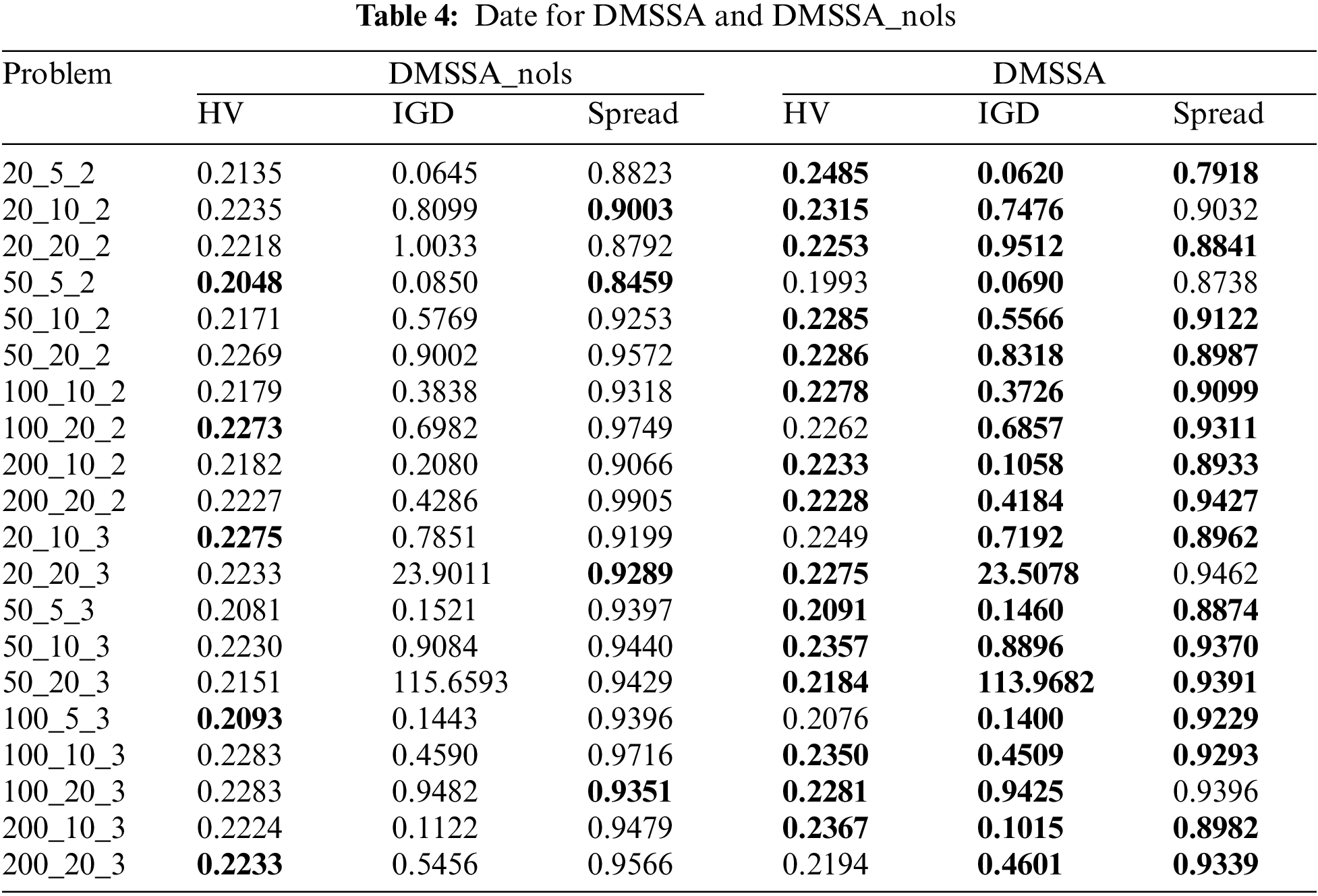
To validate the effectiveness of the local search strategy, DMSSA is compared with DMSSA without local search (referred to as DMSSA_nols). For each problem, the average results of HV, IGD, and Spread are shown in Table 4, with bold values indicating the optimal results. DMSSA achieves 15 HV values, 16 Spread values, and all IGD values outperform DMSSA_nols. This indicates that DMSSA discovers a larger set of non-dominated solutions, and the convergence and distribution of the solutions are enhanced. In conclusion, the local search strategy maximizes the utilization of problem attributes, enabling flexible exploration of potential solutions.

5.6 Effectiveness of Dynamic Predator Strategy Based on Q-Learning

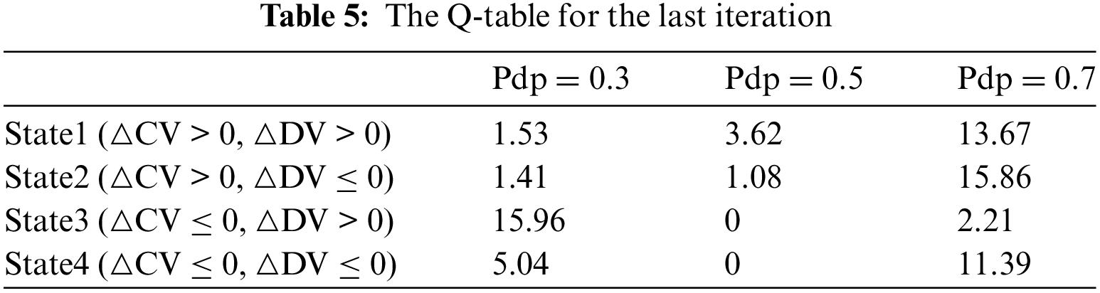
To demonstrate the effectiveness of the dynamic predator strategy based on Q-learning, Fig. 12 illustrates the convergence curves of CV and DV on the 20_5_2 problem. In the figure, each trough-to-peak cycle can be thought of as one period. Initially, multiple strategies collaborate during the iteration, leading to a rapid convergence of the population and a significant decrease in CV. During the search process, Q-learning continuously selects optimal parameters to increase diversity, leading to continuous fluctuations in DV. In the optimization process, the algorithm often gets trapped in local optima, but Q-learning is able to continuously select optimal parameters to aid its getting away from local optima. In later iterations, DV shows an upward trend of fluctuation, indicating an increasing population diversity. Table 5 provides the Q-table for the last iteration. In the early iterations, a larger Pdp is needed to increase diversity. During the iteration, to hasten the algorithm’s convergence, it is necessary to continuously decrease Pdp to guide individuals towards better individuals. However, blindly approaching the top individuals can cause the algorithm to get caught in local optima, and in such cases, it is necessary to increase Pdp to enhance population diversity. The data in Table 5 indicates that in the last iteration, Pdp = 0.3, which means Q-learning can continuously guide individuals towards excellent individuals in the later stages. In summary, the predator adaptation strategy based on Q-learning developed in this study can dynamically select optimal parameters at each state.

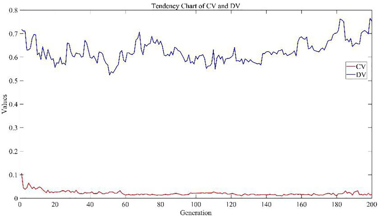
Figure 12: Change tendency graph of convergence and diversity

5.7 Comparison with Other Algorithms

To further demonstrate the outperformance of DMSSA, it is compared with classical discrete multi-objective evolutionary algorithms (MOEAs): (1) General MOEAs: NSGA-II [46], MOEA/D [48], PESA2 [49]. (2) Famous MOEAs proposed recently: AR-MOEA [50], TSNSGA-II [51]. (3) The algorithm specifically designed for DHPFSP-VPS, BRCE [26]. All algorithms have a population size (ps) of 100. The mutation probability for NSGA-II, MOEA/D, PESA2, TSNSGA-II and BRCE is set to 0.2, and the crossover probability is set to 1.0. The number of neighborhoods for MOEA/D and AR-MOEA is 10. The experiments are conducted independently, with each algorithm running 20 times on the same experimental platform. All algorithms terminate when the CPU time reaches 0.5 * n s.

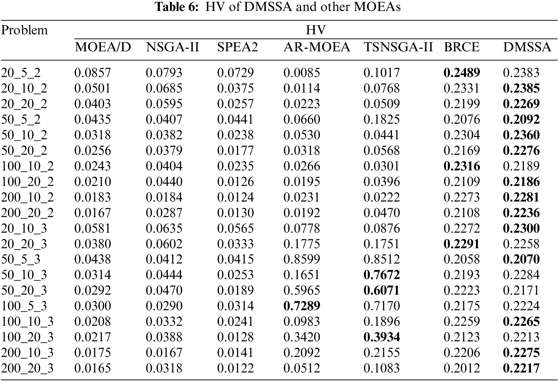
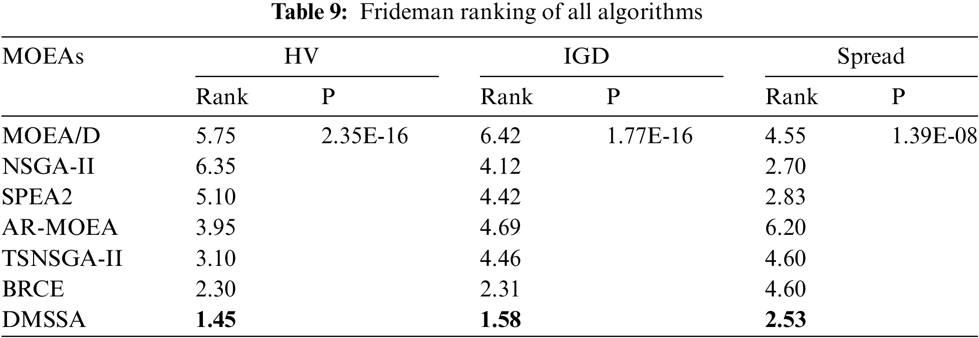
Tables 6–8 summarize the average HV, IGD, and Spread values obtained by all algorithms on the 20 problems. The bold values indicate the best results. As shown in Tables 5 and 6, DMSSA outperforms all other algorithms significantly, achieving better HV and IGD values, indicating superior overall performance and diversity. However, DMSSA performs relatively worse than BRCE in terms of HV on 4 problems and IGD on 6 problems. This is because BRCE utilizes an excellent dual-population cooperation strategy, resulting in better solution sets in a few problems. Overall, this outcome is deemed acceptable. Regarding the Spread metric presented in Table 8, DMSSA achieves the highest number of optimal solutions, ranking first, followed by NSGA-II, suggesting that the Pareto solutions obtained by DMSSA exhibit the best distribution. Table 9 presents the Friedman rank test results for all MOEAs with a significance level of 0.05. DMSSA ranks first in all metrics, and the p-values are all below 0.05, signifying the significant superiority of DMSSA over all compared algorithms.

In order to demonstrate the energy-efficient effect of DMSSA more intuitively, Fig. 13 provides a graphical representation of the PF. Two problems with varying numbers of factories are chosen to verify the efficacy of DMSSA. The figure illustrates that DMSSA can generate solutions with a uniform distribution, explore a wider range of solutions, and discover a greater number of solutions on both ends. Fig. 13 presents the set of nondominated solutions found by all algorithms running 20 times on the 20_5_2 instance and 200_10_3 instances, which strongly illustrates that the non-dominated solution set found by DMSSA can better explore the frontier, and the number and distribution of solutions are better. The lowest energy consumption of DMSSA finding solutions (829, 9544.37) is the most energy-efficient, which is 1.37% less than the lowest energy consumption of BRCE (784, 9677.23), which is the second most energy efficient, and 2.22% less than the lowest energy consumption of MOEA/D (846, 9761.43), which is the third most energy efficient. Around the completion time 3500 In Fig. 13, the points found by DMSSA are (3496.09, 239556), the points found by SPEA2 are (3504.46, 245153), and the points found by BRCE are (3495.55, 249051). It can be seen that DMSSA saves 2.28% and 3.81% energy than SPEA2 and BRCE respectively when the completion time is close. Through the analysis of the time complexity, DMSSA is comparable to other commonly used metaheuristic algorithms. Moreover, compared to other algorithms, DMSSA can always find scheduling schemes with even lower TEC. The majority of solutions discovered by DMSSA exhibit higher efficiency and superiority compared to those found by other algorithms, providing further evidence of the effectiveness of the speed control energy-efficient strategy.

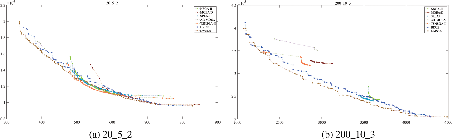
Figure 13: Pareto Frontier obtained by different algorithms

The excellent results of DMSSA are due to the synergy among all the strategies employed. The initial solutions’ quality is improved by the effective hybrid initialization method, as detailed in Section 5.3. Furthermore, the improved population ranking system and position update mechanism enable more efficient solution space exploration. Experimental outcomes, as discussed in Section 5.4, have demonstrated that the local search strategy substantially enhances the algorithm’s overall performance. The dynamic predator strategy based on Q-learning effectively improves the distribution and convergence of solutions, as described in Section 5.5. The comparative results with other algorithms indicate that DMSSA exhibits outstanding performance, and the proposed speed control energy-efficient strategy effectively reduces TEC.

In conclusion, the experimental dates validate that DMSSA outperforms other MOEAs in all cases. The superiority of DMSSA is statistically significant across all scenarios. Therefore, DMSSA is an effective method for addressing the energy-efficient DHPFSP-VPS problem.

6  Conclusion

This paper proposes a discrete multi-objective squirrel search algorithm aimed at solving the distributed heterogeneous permutation flowshop problem with variable processing speed (DHPFSP-VPS). Firstly, four initialization methods are designed based on the two optimization objectives. Secondly, six local search strategies are developed based on the characteristics of the three-stage encoding. Concurrently, improvements are made to the population ranking system and position update mechanism of SSA to better suit the characteristics of DHPFSP-VPS and enhance its search process. Furthermore, the predator strategy based on Q-learning dynamically selects optimal parameters to balance global exploration and local exploitation, thereby improving the convergence and distribution of the Pareto solution set. Finally, two speed control energy-efficient strategies are designed to reduce idle time and decrease TEC. Experimental results on 20 problems validate the effectiveness of each strategy. Comparative experiments with other algorithms indicate the outstanding performance of the proposed DMSSA in solving DHPFSP-VPS.

However, there are several aspects of work in this field that deserve further research. It would be significant to apply DMSSA to practical industrial difficulties based on the real-world manufacturing context. Moreover, in terms of the problem model, it is also possible to consider more factors, such as processing delays and machine malfunctions. Furthermore, dynamic scheduling scenarios should be considered to effectively accommodate the dynamic nature of real-world production.

Acknowledgement: Not applicable.

Funding Statement: This work was in part supported by the Key Research and Development Project of Hubei Province (Nos. 2020BAB114 and 2023BAB094).

Author Contributions: The authors confirm contribution to the paper as follows: study conception and design: Liang Zeng; data collection: Ziyang Ding; analysis and interpretation of results: Shanshan Wang; draft manuscript preparation and manuscript proofreading: Junyang Shi. All authors reviewed the results and approved the final version of the manuscript.

Availability of Data and Materials: Data is available on request from the authors. The data that support the findings of this study are available from the corresponding author, Shanshan Wang, upon reasonable request.

Ethics Approval: Not applicable.

Conflicts of Interest: The authors declare that they have no known competing financial interests or personal relationships that could have appeared to influence the work reported in this paper.

References

1. S. M. Johnson, “Optimal two-and three-stage production schedules with setup times included,” Nav. Res. Logist. Q., vol. 1, no. 1, pp. 61–68, 1954. doi: 10.1002/NAV.3800010110. [Google Scholar] [CrossRef]

2. M. R. Garey, D. S. Johnson, and R. Sethi, “The complexity of flowshop and jobshop scheduling,” Math. Oper. Res., vol. 1, no. 2, pp. 117–129, May 1976. doi: 10.1287/moor.1.2.117. [Google Scholar] [CrossRef]

3. C. N. Wang, G. Andrew Porter, C. C. Huang, V. Tinh Nguyen, and S. Tam Husain, “Flow-shop scheduling with transportation capacity and time consideration,” Comput. Mater. Contin., vol. 70, no. 2, pp. 3031–3048, 2022. doi: 10.32604/cmc.2022.020222. [Google Scholar] [CrossRef]

4. F. T. S. Chan, S. H. Chung, and P. L. Y. Chan, “An adaptive genetic algorithm with dominated genes for distributed scheduling problems,” Expert Syst. Appl., vol. 29, pp. 364–371, 2005. doi: 10.1016/j.eswa.2005.04.009. [Google Scholar] [CrossRef]

5. A. Toptal and I. Sabuncuoglu, “Distributed scheduling: A review of concepts and applications,” Int. J. Prod. Res., vol. 48, no. 18, pp. 5235–5262, Sep. 2010. doi: 10.1080/00207540903121065. [Google Scholar] [CrossRef]

6. B. Naderi and R. Ruiz, “The distributed permutation flowshop scheduling problem,” Comput. Oper. Res., vol. 37, pp. 754–768, 2010. doi: 10.1016/j.cor.2009.06.019. [Google Scholar] [CrossRef]

7. J. Gao and R. Chen, “A hybrid genetic algorithm for the distributed permutation flowshop scheduling problem,” Int. J. Comput. Intell. Syst., vol. 4, no. 4, pp. 497–508, 2011. doi: 10.1080/18756891.2011.9727808. [Google Scholar] [CrossRef]

8. J. Gao, R. Chen, and W. Deng, “An efficient tabu search algorithm for the distributed permutation flowshop scheduling problem,” Int. J. Prod. Res., vol. 51, no. 3, pp. 641–651, 2013. doi: 10.1080/00207543.2011.644819. [Google Scholar] [CrossRef]

9. A. P. Rifai, H. T. Nguyen, and S. Z. M. Dawal, “Multi-objective adaptive large neighborhood search for distributed reentrant permutation flow shop scheduling,” Appl. Soft Comput., vol. 40, pp. 42–57, 2016. doi: 10.1016/j.asoc.2015.11.034. [Google Scholar] [CrossRef]

10. S. W. Lin, K. C. Ying, and C. Y. Huang, “Minimising makespan in distributed permutation flowshops using a modified iterated greedy algorithm,” Int. J. Prod. Res., vol. 51, no. 16, pp. 5029–5038, 2013. doi: 10.1080/00207543.2013.790571. [Google Scholar] [CrossRef]

11. W. Shao, D. Pi, and Z. Shao, “A pareto-based estimation of distribution algorithm for solving multiobjective distributed nowait flow-shop scheduling problem with sequence-dependent setup time,” IEEE Trans. Autom. Sci. Eng., vol. 16, no. 3, pp. 1344–1360, 2019. doi: 10.1109/TASE.2018.2886303. [Google Scholar] [CrossRef]

12. C. Lu, Y. Huang, L. Meng, L. Gao, B. Zhang and J. Zhou, “A pareto-based collaborative multi-objective optimization algorithm for energy-efficient scheduling of distributed permutation flowshop with limited buffers,” Robot. Comput. Integr. Manuf., vol. 74, 2022, Art. no. 102277. doi: 10.1016/j.rcim.2021.102277. [Google Scholar] [CrossRef]

13. F. Zhao, D. Shao, L. Wang, T. Xu, and N. Zhu, “Jonrinaldi, an effective water wave optimization algorithm with problemspecific knowledge for the distributed assembly blocking flow-shop scheduling problem,” Knowl.-Based Syst., vol. 243, 2022, Art. no. 108471. doi: 10.1016/j.knosys.2022.108471. [Google Scholar] [CrossRef]

14. R. Ruiz, Q. K. Pan, and B. Naderi, “Iterated Greedy methods for the distributed permutation flowshop scheduling problem,” Omega, vol. 83, pp. 213–222, 2019. doi: 10.1016/j.omega.2018.03.004. [Google Scholar] [CrossRef]

15. H. Bargaoui, O. Belkahla, and K. Ghédira, “A novel chemical reaction optimization for the distributed permutation flowshop scheduling problem with makespan criterion,” Comput. Ind. Eng., vol. 111, pp. 239–250, 2017. doi: 10.1016/j.cie.2017.07.020. [Google Scholar] [CrossRef]

16. J. Li, S. Bai, P. Duan, H. Sang, Y. Han and Z. Zheng, “An improved artificial bee colony algorithm for addressing distributed flow shop with distance coefficient in a prefabricated system,” Int. J. Prod. Res., vol. 57, no. 22, pp. 6922–6942, 2019. doi: 10.1080/00207543.2019.1571687. [Google Scholar] [CrossRef]

17. J. Lin, Z. J. Wang, and X. Li, “A backtracking search hyper-heuristic for the distributed assembly flow-shop scheduling problem,” Swarm Evol. Comput., vol. 36, pp. 124–135, 2017. doi: 10.1016/j.swevo.2017.04.007. [Google Scholar] [CrossRef]

18. M. Akbar and T. Irohara, “Scheduling for sustainable manufacturing: A review,” J. Clean.Prod., vol. 205, pp. 866–883, 2018. doi: 10.1016/j.jclepro.2018.09.100. [Google Scholar] [CrossRef]

19. IEA, “Worldwide trends in energy use and efficiency: Key insights from iea indicator analysis,” 2008. Accessed: Aug. 11, 2024. [Online]. Available: http://sa.indiaenvironmentportal.org.in/files/Indicators_2008.pdf [Google Scholar]

20. J. Wang and L. Wang, “A knowledge-based cooperative algorithm for energy-efficient scheduling of distributed flow-shop,” IEEE Trans. Syst., Man, Cybern.: Syst., vol. 50, no. 5, pp. 1805–1819, 2018. doi: 10.1109/TSMC.2017.2788879. [Google Scholar] [CrossRef]

21. J. Wang and L. Wang, “A cooperative memetic algorithm with feedback for the energy-aware distributed flow-shops with flexible assembly scheduling,” Comput. Ind. Eng., vol. 168, 2022, Art. no. 108126. doi: 10.1016/j.cie.2022.108126. [Google Scholar] [CrossRef]

22. Y. Li, Q. Pan, K. Gao, M. F. Tasgetiren, B. Zhang and J. Li, “A green scheduling algorithm for the distributed flowshop problem,” Appl. Soft Comput., vol. 109, 2021, Art. no. 107526. doi: 10.1016/j.asoc.2021.107526. [Google Scholar] [CrossRef]

23. F. Zhao, R. Ma, and L. Wang, “A self-learning discrete jaya algorithm for multiobjective energy-efficient distributed no-idle flow-shop scheduling problem in heterogeneous factory system,” IEEE Trans. Cybern., vol. 52, no. 12, pp. 12675–12686, Dec. 2022, doi: 10.1109/TCYB.2021.3086181. [Google Scholar] [PubMed] [CrossRef]

24. A. M. Fathollahi-Fard, L. Woodward, and O. Akhrif, “Sustainable distributed permutation flow-shop scheduling model based on a triple bottom line concept,” J. Ind. Inf. Integr., vol. 24, 2021, Art. no. 100233. doi: 10.1016/j.jii.2021.100233. [Google Scholar] [CrossRef]

25. J. Jiang, Y. An, Y. Dong, J. Hu, Y. Li and Z. Zhao, “Integrated optimization of non-permutation flow shop scheduling and maintenance planning with variable processing speed,” Reliab. Eng. Syst. Safety, vol. 234, 2023, Art. no. 109143. doi: 10.1016/j.ress.2023.109143. [Google Scholar] [CrossRef]

26. K. Huang, R. Li, W. Gong, R. Wang, and H. Wei, “BRCE: bi-roles co-evolution for energy-efficient distributed heterogeneous permutation flow shop scheduling with flexible machine speed,” Complex Intelli. Syst, vol. 9, pp. 4805–4816, 2023. doi: 10.1007/s40747-023-00984-x. [Google Scholar] [CrossRef]

27. G. Wang, L. Gao, X. Li, P. Li, and M. F. Tasgetiren, “Energy-efficient distributed permutation flow shop scheduling problem using a multi-objective whale swarm algorithm,” Swarm Evol. Comput., vol. 57, 2020, Art. no. 100716. doi: 10.1016/j.swevo.2020.100716. [Google Scholar] [CrossRef]

28. P. Perez-Gonzalez and J. M. Framinan, “A review and classification on distributed permutation flowshop scheduling problems,” Eur. J. Oper. Res., vol. 312, no. 1, pp. 1–21, 2023. doi: 10.1016/j.ejor.2023.02.001. [Google Scholar] [CrossRef]

29. M. Jain, V. Singh, and A. Rani, “A novel nature-inspired algorithm for optimization: Squirrel search algorithm,” Swarm Evol. Comput., vol. 44, pp. 148–175, 2019. doi: 10.1016/j.swevo.2018.02.013. [Google Scholar] [CrossRef]

30. T. Zheng and W. Luo, “An improved squirrel search algorithm for optimization,” Complexity, vol. 2019, no. 1, 2019, Art. no. 153. doi: 10.1155/2019/6291968. [Google Scholar] [CrossRef]

31. P. Wang, Y. Kong, X. He, M. Zhang, and X. Tan, “An improved squirrel search algorithm for maximum likelihood DOA estimation and application for MEMS vector hydrophone array,” IEEE Access, vol. 7, pp. 118343–118358, 2019. doi: 10.1109/ACCESS.2019.2936823. [Google Scholar] [CrossRef]

32. E. S. M. El-Kenawy et al., “Advanced meta-heuristics, convolutional neural networks, and feature selectors for efficient COVID-19 X-ray chest image classification,” IEEE Access, vol. 9, pp. 36019–36037, 2021. doi: 10.1109/ACCESS.2021.3061058. [Google Scholar] [PubMed] [CrossRef]

33. V. P. Sakthivel and P. D. Sathya, “Multi-area economic environmental dispatch using multi-objective squirrel search algorithm,” Evol. Syst., vol. 13, no. 2, pp. 183–199, 2022. doi: 10.1007/s12530-021-09366-5. [Google Scholar] [CrossRef]

34. Y. Wang and J. Han, “A FJSSP method based on dynamic multi-objective squirrel search algorithm,” Int. J. Antennas Propag., vol. 2021, pp. 1–19, 2021. doi: 10.1155/2021/6062689. [Google Scholar] [CrossRef]

35. B. Jaishankar, S. Vishwakarma, P. Mohan, A. K. S. Pundir, I. Patel and N. Arulkumar, “Blockchain for securing healthcare data using squirrel search optimization algorithm,” Intell. Autom. Soft Comput., vol. 32, no. 3, pp. 1815–1829, 2022. doi: 10.32604/iasc.2022.021822. [Google Scholar] [CrossRef]

36. D. Guha, P. K. Roy, and S. Banerjee, “Frequency control of a wind-diesel-generator hybrid system with squirrel search algorithm tuned robust cascade fractional order controller having disturbance observer integrated,” Elect. Power Compon. Syst., vol. 50, no. 14–15, pp. 814–839, 2022. doi: 10.1080/15325008.2022.2141925. [Google Scholar] [CrossRef]

37. K. Ishwarya and A. A. Nithya, “Squirrel search optimization with deep convolutional neural network for human pose estimation,” Comput. Mater. Contin., vol. 74, no. 3, pp. 6081–6099, 2023. doi: 10.32604/cmc.2023.034654. [Google Scholar] [CrossRef]

38. D. Maden, E. Çelik, E. H. Houssein, and G. Sharma, “Squirrel search algorithm applied to effective estimation of solar PV model parameters: A real-world practice,” Neural Comput. Appl., vol. 35, no. 18, pp. 13529–13546, 2023. doi: 10.1007/s00521-023-08451-x. [Google Scholar] [CrossRef]

39. M. Wu, D. Yang, Z. Yang, and Y. Guo, “Sparrow search algorithm for solving flexible jobshop scheduling problem,” in Y. Tan, Y. Shi (eds.), Advances in Swarm Intelligence., Cham: Springer, 2021, vol. 12689. doi: 10.1007/978-3-030-78743-1_13. [Google Scholar] [CrossRef]

40. Y. An, X. Chen, K. Gao, Y. Li, and L. Zhang, “Multiobjective flexible job-shop rescheduling with new job insertion and machine preventive maintenance,” IEEE Transact Cybern, vol. 53, no. 5, pp. 3101–3113, May 2023. doi: 10.1109/TCYB.2022.3151855. [Google Scholar] [PubMed] [CrossRef]

41. C. J. C. H. Watkins and P. Dayan, “Technical note: Q-learning,” Mach. Learn., vol. 8, no. 3, pp. 279–292, 1992. doi: 10.1023/A:1022676722315. [Google Scholar] [CrossRef]

42. X. Zhang, K. Zhao, L. Wang, Y. Wang, and Y. Niu, “An improved squirrel search algorithm with reproductive behavior,” IEEE Access, vol. 8, pp. 101118–101132, 2020. doi: 10.1109/ACCESS.2020.2998324. [Google Scholar] [CrossRef]

43. R. Li, W. Gong, and C. Lu, “A reinforcement learning based RMOEA/D for bi-objective fuzzy flexible job shop scheduling,” Expert Syst. Appl., vol. 203, 2022, Art. no. 117380. doi: 10.1016/j.eswa.2022.117380. [Google Scholar] [CrossRef]

44. L. While, P. Hingston, L. Barone, and S. Huband, “A faster algorithm for calculating hypervolume,” IEEE Trans. Evol. Comput., vol. 10, no. 1, pp. 29–38, 2006. doi: 10.1109/TEVC.2005.851275. [Google Scholar] [CrossRef]

45. C. H. R. Jethmalani, S. P. Simon, K. Sundareswaran, P. S. R. Nayak, and N. P. Padhy, “Auxiliary hybrid PSO-BPNN-based transmission system loss estimation in generation scheduling,” IEEE Trans. Ind. Inform., vol. 13, pp. 1692–1703, 2017. doi: 10.1109/TII.2016.2614659. [Google Scholar] [CrossRef]

46. K. Deb, A. Pratap, S. Agarwal, and T. Meyarivan, “A fast and elitist multiobjective genetic algorithm: Nsga-ii,” IEEE Trans. Evol. Comput., vol. 6, no. 2, pp. 182–197, 2002. doi: 10.1109/4235.996017. [Google Scholar] [CrossRef]

47. R. C. Van, “Design of experiments using the taguchi approach: 16 steps to product and process improvement,” Technometrics, vol. 44, no. 3, p. 289, 2002. doi: 10.1198/004017002320256440. [Google Scholar] [CrossRef]

48. Q. Zhang and L. Hui, “MOEA/D: A multiobjective evolutionary algorithm based on decomposition,” IEEE Trans. Evol. Comput., vol. 11, no. 6, pp. 712–731, 2007. doi: 10.1109/TEVC.2007.892759. [Google Scholar] [CrossRef]

49. E. Zitzler, M. Laumanns, and L. Thiele, “SPEA2: Improving the strength pareto evolutionary algorithm,” in TIK Report, ETH Zurich, Computer Engineering and Networks Laboratory, 2001, vol. 103. doi: 10.3929/ethz-a-004284029. [Google Scholar] [CrossRef]

50. B. Li, K. Tang, J. Li, and X. Yao, “Stochastic ranking algorithm for many-objective optimization based on multiple indicators,” IEEE Trans. Evol. Comput., vol. 20, no. 6, pp. 924–938, 2016. doi: 10.1109/TEVC.2016.2549267. [Google Scholar] [CrossRef]

51. F. Ming, W. Gong, and L. Wang, “A two-stage evolutionary algorithm with balanced convergence and diversity for many-objective optimization,” IEEE Trans. Syst., Man, Cybern.: Syst., vol. 52, no. 10, pp. 6222–6234, 2022. doi: 10.1109/TSMC.2022.3143657. [Google Scholar] [CrossRef]