Elevating Localization Accuracy in Wireless Sensor Networks: A Refined DV-Hop Approach

1  Introduction

Node localization is a crucial element in various WSN applications. Numerous algorithms have been designed [1,2] to determine the precise positions of SNs. However, the role of GPS in this process is often hindered by environmental or hardware constraints [3], dense urban environments [4], and mountain regions [4]. In these situations, the absence of GPS signals requires the development of cost-effective and efficient localization methods [5]. The diversity of range-based [6] algorithms in WSNs, which calculate the distance between nodes, is evident in their various types: received signal strength (RSS), time difference of arrival (TDOA), time of arrival (TOA), and angle of arrival (AOA). On the other hand, the range-free algorithms [7] include the Distance Vector Hop (DV-Hop) algorithm and the Centroid and Amorphous algorithm. The range-free algorithms require knowledge of the connectivity between nodes without any reliance on additional hardware [8]. DV-Hop is a range-free technique that has the added benefit of being low-cost and easy to implement, without any extra hardware requirements for wireless sensor network nodes [9–11]. In recent years, many researchers have proposed enhanced DV-Hop techniques to address the localization accuracy issue [11–13]. Despite advancements, existing methods still have critical shortcomings that motivate this research:

1)   Optimum anchor node selection: Many DV-Hop techniques fail to select optimized anchor nodes, leading to significant localization inaccuracy [13,9].

2)   Assistant anchor node selection: Enhancements often select all localized nodes as assistant anchor nodes, impacting localization accuracy. The ratio of nodes involved in localization is not sufficiently addressed [14,15].

3)   Average hop distance calculation: Existing methods lack a refined average hop distance calculation, leading to imprecise localization. Incorporating a correction factor is essential for improving accuracy [9].

In this work, we address two issues related to localization accuracy. First, we explore selecting the most appropriate anchor nodes to enhance localization accuracy. Second, our research explores methods to enhance localization by upgrading localized nodes to serve as assistant anchor nodes since the proportion of anchor nodes directly impacts the accuracy of localization. We suggest further integrating a correction factor for average hop distance to refine localization accuracy. The key contributions of our study are summarized as follows:

1)   We are introducing AS-IDV-Hop, a method to select the most appropriate connected anchor node, enhancing localization accuracy.

2)   It proposes an upgrading technique to elevate localized nodes to assistant anchor nodes, bolstering localization accuracy. This is particularly crucial as the proportion of anchor nodes influences accuracy.

3)   We introduce an average hop distance calculation method that incorporates a correction factor accounting for the precise positions of anchor nodes. This refinement ensures more accurate localization outcomes.

Furthermore, the proposed technique removes the collinearity phenomena from the anchors that play a part in the localization process. The proposed algorithm’s first stage is similar to the traditional algorithm but involves selecting anchor and assistant anchor nodes for the localization process. In the algorithm, the average hop distance is adjusted in the second step, followed by position estimation in the third step [16]. The paper structure is as follows. Related work is discussed in Section 2. Section 3 presents traditional DV-Hop and a proposed algorithm called AS IDV-Hop. Section 4 illustrates the effectiveness of the suggested approach through simulation results. The findings are accomplished in Section 5.

2  Literature Review

This section describes the enhanced DV-Hop localization model and provides an overview of two existing localization methods. Connectivity information and anchors’ position are used to estimate the nodes’ location in range-free schemes [13,14]. The proportion of anchor nodes can be adjusted based on the network’s connectivity [15]. An unknown node’s position estimation with anchors requires efficient utilization of anchors and network resources [17]. The selection process of anchor nodes for the localization is based on maximum connectivity because these groups of anchor nodes cover all the unknown nodes. The sub problem that usually causes a negative impact on localization accuracy is the collinearity phenomenon [18], the accuracy of localization is impacted when all nodes are aligned in a straight line, which influences the localization process.

An enhanced version of DV-Hop has been created to effectively handle the mobility of anchor nodes and the movement of unknown nodes. Through anchor coordination, the algorithm forms the backbone called Minimum Connected Dominating Set (MCDS) [19,20] of the network, efficiently utilizing network resources to estimate the positions of unknown nodes. The algorithm’s primary goal is to use anchor nodes efficiently. The Friis free space propagation model calculates the distance between unknown and anchor nodes to account for mobility. Maximum connected anchor nodes to unknown nodes within one hop distance are selected as the network’s backbone. However, the propagation model assumes a straight-line link between the transmitter and receiver, which is only sometimes the case due to environmental factors. The selection of anchor nodes does not consider the degree of collinearity. If the nodes are collinear, it can affect the position estimation accuracy, and all nodes may not be within one hop away from the anchor nodes in the real scenario [17].

Sparse connectivity decreases the probability of accurate localization in a network [21]. Range-free localization algorithms are less expensive and simpler to implement, but their accuracy is often poor due to the limited number of anchors in networks. To address this challenge, various improved schemes based on DV hop and RSSI have been introduced to estimate the node positions [22]. The density of anchors is a crucial parameter in range-free schemes [23]. To localize all the nodes in a network using range-free schemes, 20%–40% anchors are required [22]. Selecting the right group of assistant anchors participating in the location estimation can significantly impact localization accuracy. A proposed solution uses an error control mechanism that relies on specific geometric features to prevent errors from spreading and accumulating in a network. This mechanism selects which nodes should participate in localization to estimate unknown nodes’ locations. However, substantial anchors must be deployed to ensure that every unknown node in an extensive network can be located. Unfortunately, adding extra anchor nodes can result in additional expenses related to hardware, deployment, and maintenance [22].

In iterative localization, the localized nodes in the first round successfully become assistant anchor nodes. Due to cost constraints, the key factor determining network quality is energy utilization. Localization needs to be achieved with a smaller number of iterations [24]. It is supposed that, in the DV-Hop scheme, nearby anchors provide more accuracy in localization. However, they do not provide accurate location estimation if the anchors are near other anchors. Regarding location estimation precision, hop size from some anchor nodes has more influence [25].

Cao et al. [11] proposed a technique in which the hop count mechanism is modified from an integer value to a decimal value. This is achieved by altering the communication range of anchor nodes through conciliation between nodes. By refining the hop count in this way, the accuracy of the distance between anchor nodes and unknown nodes is improved. Sun et al. [26] proposed a technique that incorporates the 2D hyperbolic algorithm in the third step of the traditional DV-Hop algorithm to enhance localization accuracy. Wang et al. [27] proposed a technique in which cross-domain information is used to estimate the distance between anchor nodes and unknown nodes, and multiple anchor nodes are used for localization. The metric of hop loss is introduced to enhance the localization accuracy and minimize the difference between actual position and estimated position and Euclidean distance loss. The hop loss is incorporated into the algorithm, and the loss of Euclidean distance is calculated using the proposed technique.

A subset-based anchor node selection method is proposed to decrease the localization error [9]. A new strategy is proposed to decrease the error in coordination estimation of unknown modes. The improved DV-Hop concludes the subset of anchor nodes, improves hope distance, and concludes the subset broadcast to the unknown nodes. The MOANS DV-Hop does not consider the collinearity phenomenon for improvement in localization accuracy. Collinear anchor nodes have a significant impact on location estimation.

Numerous factors affect average hop distance (AHD) and lead to the multipath effect, such as walls, equipment, human beings, and electromagnetic wave propagation. Walls and other structures cause a fluctuation in RSSI [28]. Interference affects positioning accuracy. A proposed improved DV-Hop hybrid that uses the correction of hop distance to consider the relation between localization accuracy and network topology. The proposed method uses the RSSI value within a single hop to determine the distance between anchor nodes and unknown nodes. The correction value is added to the original hop distance between unknown and anchor nodes to decrease the distance error between them. However, the coverage and increased accuracy of the localized nodes still need to be upgraded to assistant anchor nodes [21].

Li et al. [29] proposed a non-ranging node localization method for irregular regions, utilizing the PSO algorithm and anchor node pair selection. Phoemphon et al. [30] introduced a hybrid localization model using node segmentation and improved PSO for WSNs. Han et al. [31] enhanced accuracy through RSSI value conversion and DV-Hop with differential evolution (DE) algorithms to address average hop distance errors.

In their study, Kaur et al. [32] introduced a weighted centroid localization algorithm for randomly deployed Wireless Sensor Networks (WSNs). Kanwar et al. [33] presented an innovative multi-hop algorithm known as ML-EN, designed to address challenges posed by unevenly distributed nodes. Kanwar et al. [34] developed an accurate deep learning (DL) method for DV-Hop localization in the Internet of Things (IoT) using the whale optimization algorithm (WOA). This approach utilizes a deep neural network (DNN), and simulations demonstrate its superior positional accuracy. Additionally, the proposed non-ranging method may offer greater adaptability to the diversity and complexity of real-world WSN environments.

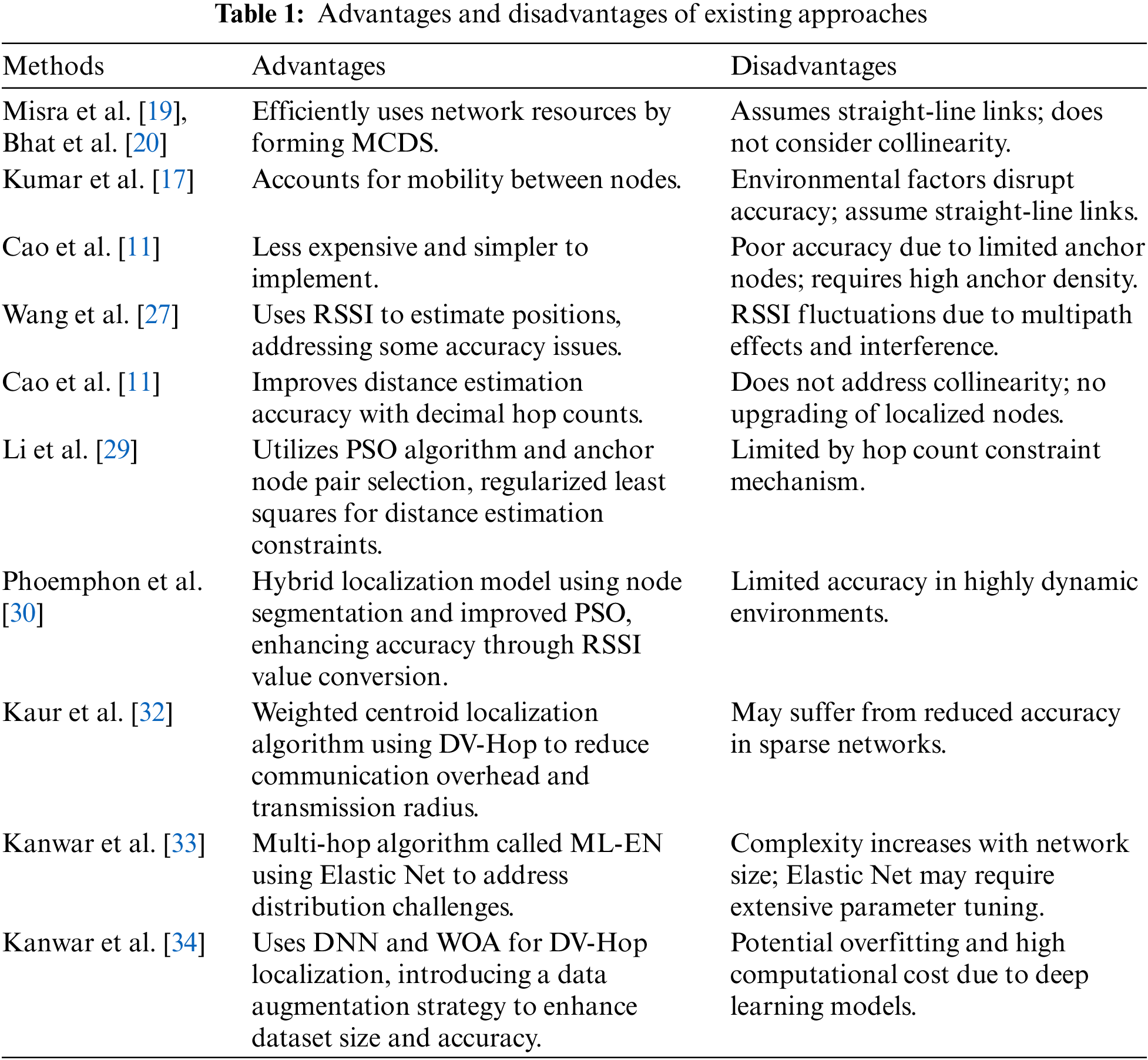
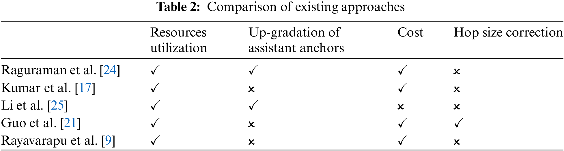
Table 1 compares the advantages and disadvantages of existing approaches, and Table 2 compares research quality across four metrics: resource utilization, upgrading of assistant anchor nodes, cost, and correction of hop size. It is worth noting that current studies only address a subset of these parameters.

3  Design of Proposed Solution

The proposed solution includes the fundamentals of the traditional DV-Hop in the first segment and anchors an optimum set-based localization procedure in the second segment. The second section includes the elimination of the collinear anchor nodes from the localization process and the construction process of the backbone of the network by pruning the less connected anchor nodes. The connection between these subsections involves a systematic approach to hop counting, average hop distance calculation, MCDS construction, and optimization through pruning. Each subsection contributes to the overall localization process, ensuring efficiency and accuracy in estimating the coordinates of unknown nodes. Fig. 1 depicts the process flow of the proposed approach.

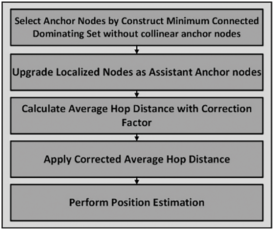
Figure 1: Workflow of the proposed method

The DV-Hop method was initially introduced in 2003 [7]. It faces several challenges related to accuracy, environmental factors, mobility, and computational overhead; DV-Hop has gained widespread adoption in several uses due to practicality, stability, simplicity, and minimal hardware necessities [35]. A concise summary of the original DV-Hop is provided [16]. There are three fundamental phases of traditional DV-Hop.

3.1 The Fundamental of DV-Hop

DV-Hop is a localization algorithm used in wireless sensor networks. In this algorithm, nodes contribute to distance estimation in a hop-by-hop approach. This algorithm is useful in situations where accurate location information is essential.

3.1.1 Hop Counting between Anchor Nodes and Unknown Nodes

Broadcasting is used to count the minimum hops among the unknown nodes and the anchor nodes. Anchor nodes (N) in the network establish a table containing the coordinates of every anchor and the corresponding number of hops from the node itself and every anchor node. In the first phase, every anchor transmits a message throughout the network, flooding information about the anchor’s location and initializing the value of the hop to one by using Eq. (1).

AnchorsNi={(Nj,LocationNj,1)}(1)

Every receiving node tracks the smallest hop value for each anchor by analyzing all the anchors it receives using Eq. (2).

MinHopsNk=min(MinHopsNk,HopsNj)(2)

Anchors with high hops values directed to specific anchors are considered outdated and disregarded. Eq. (3) ensures that every unknown node obtains the minimum hops from every anchor node.

MinHopsNk={MinHopsNkif HopsNj>MinHopsNkHopsNjotherwise(3)

The message is transmitted sequentially from one node to another, and the hop counts are recorded from every anchor to every subsequent node. Every node possesses a counting table that keeps track of the minimum hops required to reach the anchor node.

3.1.2 Estimation of Average Hop Distance from Unknown Node to Anchor Nodes

In the second phase of traditional DV-Hop, the average hop distance is determined based on the number of hops counted in the first phase. Average hop distance estimation uses Eq. (4), derived from the hop count information calculated in the first phase.

HopSizei=∑i≠j(Xi−Xj)2+(Yi−Yj)2∑i≠jhj(4)

In Eq. (4), HopSizei represents the average hop distance, Xi, Yi and Xj, Yj denote the coordinates of i and j nodes. hj indicates the hops count that are MinHopsNk.

3.1.3 Calculate the Coordinates of the Unknown Node

Assume that the coordinates of the unknown node u are represented by (y,z), while the coordinates of the i-th anchor node are represented by (yi,zi) (1≤i≤n); additionally, let di(1≤i≤n) denote the distance between the i-th anchor node and unknown node u. If a minimum of three distances that have been calculated in Step 2, the unknown node’s coordinates may be determined using Eq. (5).

(x−x1)2+(y−y1)2=d12(x−x2)2+(y−y2)2=d22..(x−xn)2+(y−yn)2=dn2(5)

3.2 Anchors Set-Based Improved DV-Hop Algorithm

Minimum Connected Dominating Set (MCDS) [36] has been introduced for anchor and assistant anchor nodes; the proposed technique is based on three phases. Firstly, searching to build a dominating set; secondly, connectors are identified; and finally, the MCDS prunes method is applied. The pruning method minimizes the size of the MCDS of assistant anchor nodes by covering all the unknown nodes. The node failure due to power constraints is also considered. In the proposed methodology, only those assistant anchors are selected to play a part in the localization process, which has maximum connectivity and is not greater than one hop away from the unknown node. The assistance anchors establish a dominant set to locate unknown and isolated unknown nodes. Pruning is used to reduce nodes’ dual occurrence and lower the dominant set’s size, thereby avoiding repetition.

Broadcast a message to calculate the connectivity of the anchor node by using a threshold value. The threshold value in the proposed methodology is two. Check the connectivity level of the node up to two hops. Within a one-hop distance, two nodes have the same level of connectivity. That is why we need to check the connectivity level for two hours. When implementing the algorithm in the simulator, try to increase the threshold value at more levels to choose the best assistant anchor node for full coverage of the localization network by considering the ratio of communication overhead. An assistant anchor node is selected based on the distance among assistant anchor nodes selected to perform the localization process, which should be as similar as possible. Also, consider the position of assistant anchor nodes; removing those assistant anchor nodes will minimize the internal angle of the triangle.

In large-scale network environments [37], irregularity of radio signals is a common phenomenon in WSNs—the obstacles in the middle of transmission cause the irregularity of radio signals. The irregularity of radio signals has a significant impact on localization accuracy and network coverage. In comparison, localization applications need high coverage and connectivity. The previously proposed technique [38] uses a log-normal shadowing path loss model to calculate the distance among the nodes. The log-normal shadow model describes the signal fading for the propagation of the signal [39]. Eq. (6) is used in the proposed methodology to calculate the distance between anchor nodes, assistant anchor nodes, and unknown nodes.

RSS(d)(dBm)=Ptr−Ploss(do)+10τlog10ddo(6)

The variable “d” represents the distance between the sending and receiving nodes. “RSS(d)” refers to the received signal power of nodes placed at a distance of “d”. “do” is the referenced distance. “Ptr” denotes the transmitting power. “Ploss(do)” represents the path loss for “do”. “τ” indicates the loss exponent in the path, and its value depends on the propagation environment. The variable Xσ′ represents the noise in RSSI, and it follows a Gaussian distribution with a mean of zero and a standard deviation of σ. The suggested technique utilizes the log-normal shadowing model to estimate the distance between unknown and coordinate nodes.

3.2.1 Collinear Anchor Nodes

Localization accuracy is influenced by the collinearity phenomenon, which occurs when nodes are aligned in a straight line during localization. If unknown nodes have two anchor nodes, an assistant anchor node collaborates to estimate their positions. Zhang et al. [18] proposed a mechanism to select anchor nodes that satisfy collinearity and threshold requirements. The proposed algorithm excludes collinear anchor nodes from the dominating set.

3.2.2 Prune Process

Sometimes, a single unknown node might be connected to more than one anchor node. A pruning method prevents redundancy and ensures that the dominating set (D) is formed with the fewest anchor nodes. It ultimately provides the MCDS as the backbone to localize the unknown nodes.

In Fig. 2a, the flow chart illustrates the complete localization process; in Fig. 2b, the flow chart illustrates the pruning process. After initialization, the minimum hop count is calculated using a traditional DV-Hop algorithm. After that, the minimum connected dominating set construction process starts. In this process, the pruning algorithm calls to prune the dominating set for the localization process on the constraint of collinearity and connectivity of the anchor nodes. In our given scenario, Fig. 3, let us consider the anchor node labeled ‘2’, which shows the highest level of connectivity with the unknown nodes, having six nodes within its range. Consequently, in the initial iteration, anchor node ‘2’ is included in the dominating set. Similarly, nodes ‘1’ and ‘3’ also join this set. Together, these anchor nodes (1, 2, and 3) effectively cover all the nearby unknown nodes. As a result, there’s no need to add anchor nodes ‘4’ and ‘5’ to the dominating set.

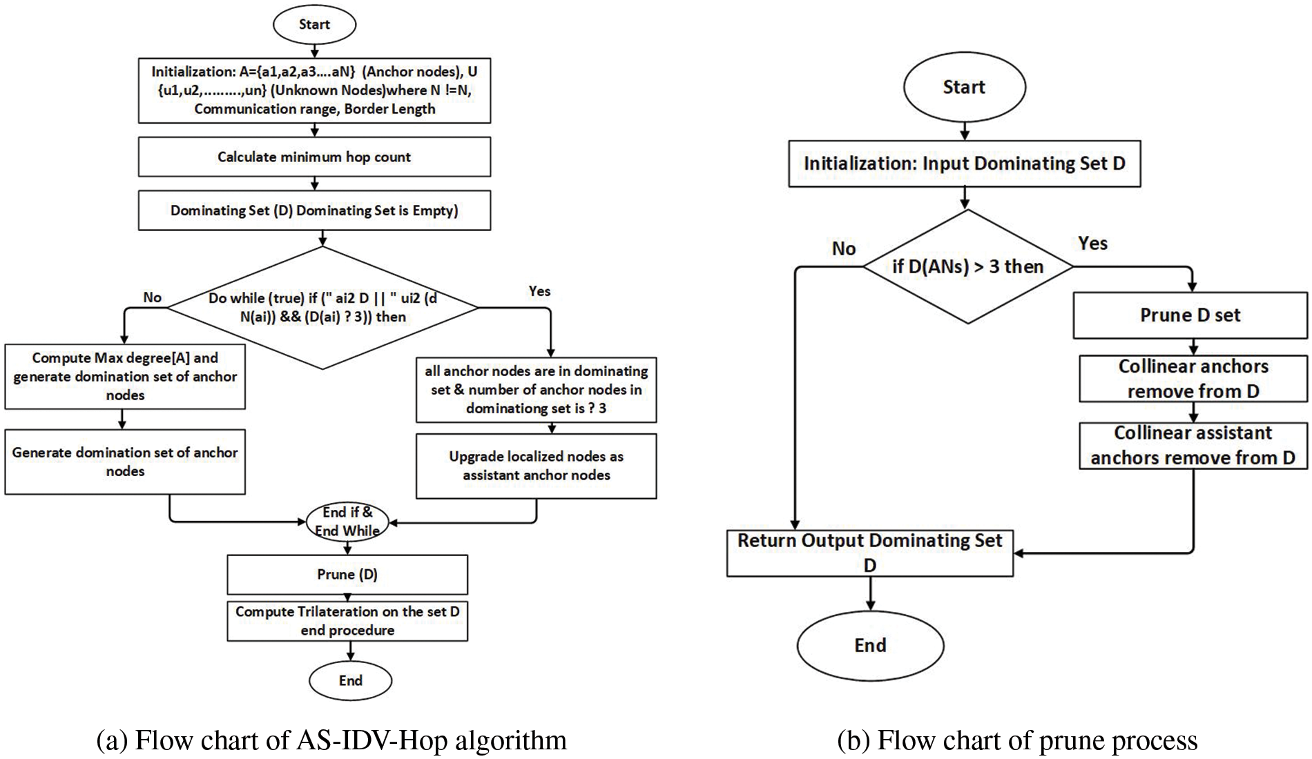
Figure 2: Flow charts of proposed DV-Hop algorithm: (a) AS-IDV-Hop algorithm, (b) prune process

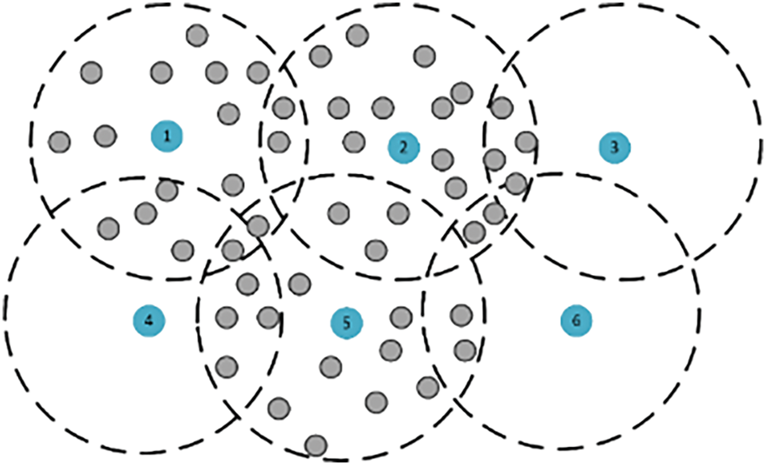
Figure 3: Minimum connected dominating set (MCDS)

The dominating set is connected and covers the minimum number of nodes; in this case, three out of the five anchor nodes are efficiently connected. This minimal selection of anchor nodes meets the trilateration’s minimum requirement, effectively covering all the unknown nodes. This property designates it as the MCDS.

Localized nodes were upgraded as assistant anchors to enhance the location estimation accuracy based on the minimum localization error of localized nodes and upgraded as assistant anchor nodes by using the RSSI-based distance because the nearest assistant anchor node of an unknown node significantly impacts location estimation—average hop distance correction made in the second step of the algorithm. Average hop distance had a significant impact on location estimation.

The average hop distance is corrected by adding a correction factor that consists of the actual location of anchor nodes and the distance between anchor and assistant anchor nodes.

hopsize=dij[dijR](7)

The distance between anchor node “i” and unknown node “j” and “R” is the communication range.

dij=(hopsize×hopsij)+α⋅norm(loci−locass,i)(8)

The aim is to improve the average hop distance by adding the correction factor in equation Eq. (8), while the hop size is calculated from Eq. (7) while α is the scaling parameter for the correction factor. “loci” is the actual location of anchor node and “locass” location of the assistant anchor node related to anchor. Average hop distance correction decreases the accumulated location estimation error and increase the location estimation accuracy.

4  Simulation and Performance Evaluation

For the simulation of the proposed methodology, the simulation area is 100 m × 100 m and 200 m × 200 m. The anchor nodes for the localization process and unknown nodes are randomly and evenly deployed. The simulation parameters [17] are listed in Table 3.

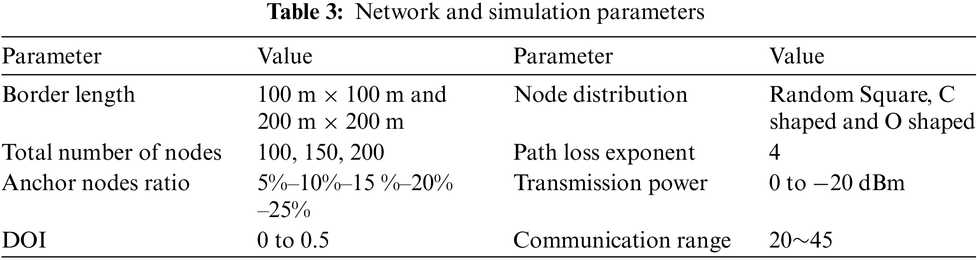
The three parameters, the number of anchor nodes, the number of unknown nodes, and the communication range, diverge after a specific range while the simulation area is not changed. In a natural environment, the node’s communication radius is unequal due to attenuation, signal direction, and node residual energy. The communication error is set to 0% to 30%.

4.1 Simulation Parameters and Performance Evaluation Metrics

For the simulation of the proposed methodology, the simulation area is 100 m × 100 m and 200 m × 200 m. The anchor nodes for the localization process and unknown nodes are randomly and evenly deployed. The simulation parameters are listed in Table 3, which is set for simulation, and the three parameters, the number of anchor nodes, the number of unknown nodes, and the communication range, diverge after a specific range. In contrast, the area of simulation is not changed. In a natural environment, the node’s communication radius is unequal due to attenuation, signal direction, and node residual energy. The communication error is set to 0% to 30%.

4.1.1 Average Localization Error

The primary performance metric of localization is ALE (Average Localization Error) calculated by Eq. (9).

ALE=∑i=1ANs−UNs(xiact−xiest)2+(yiact−yiest)2(ANs−UNs)×R(9)

In this equation, ANs denote the number of anchor nodes, UNs denotes the number of unknown nodes, while the (xiact−xiest) and (yiact−yiest) are the actual and estimated coordinates of nodes.

4.1.2 Accuracy

Accuracy (Zafari et al. [40]) is the main key to evaluating of localization techniques. To estimate how accurately a system locates the calculated objects, Sun et al. [41] provided the following Eq. (10):

γ=∑i=1Num(xitrue−xiest)2+(yitrue−yiest)2Num×R(10)

The variables (xitrue, yitrue) denote the real position of an unknown node i, whereas (xiest, yiest) indicate the estimated coordinates of the same unknown node i, as computed via localization methods. “Num” represents the total count of nodes with unknown values, whereas R is the maximum distance within which sensor nodes can communicate. Moreover, variance is calculated by using Eq. (11). σ2 is the variance, N is the number of data points, xi represents the individual data points and µ is the mean of data points.

σ2=1N∑Ni=1(xi−µ)2(11)

4.1.3 Coverage

The coverage [42] is to evaluate the localization techniques. The coverage means how many network nodes will be localized in the network. There is a need to pay attention to adding other nodes within the network after the completion of the initial localization algorithm. Coverage refers to the proportion of nodes deployed within the network, aiming to localize the entire network, regardless of the accuracy of the localization process. The proposed algorithm 99% localizes the unknown nodes.

4.1.4 Cost

The cost [40] of the localization algorithm refers to various substances such as the ratio of anchor nodes, cost of communication, computation complexity cost, consumption of energy, and special software and hardware required by every node. Ideally, the localization system should not increase the infrastructure cost. The complexity of the algorithm can be explained in big O notation which is the standard notation of complexity of computation in space and time. Need to consider how long the algorithm runs before estimating the locations of unknown nodes, and how much storage is required for those calculations. The AS-IDV-Hop algorithm, though more complex than the traditional DV-Hop algorithm [43], offers significantly improved localization accuracy. Our proposed solution strikes a balances accuracy and complexity, parallel to the findings presented by Kumar et al. [17]. In this regard, both Kumar et al.’s algorithm and our proposed algorithm exhibit similar complexities. However, it’s worth noting that the algorithm introduced by Rayavarapu et al. [9] carries a higher time complexity than our proposed approach. Proposed algorithm’s complexity is denoted as O(A2×U), where A represents the number of anchor nodes and U stands for the number of unknown nodes. We assess the algorithm’s performance based on these three factors, ratio of anchor nodes, ratio of unknown nodes and communication range of nodes in the network.

4.2 AS-IDV-Hop Algorithm Advantage

Localization accuracy is compared with three algorithms: the traditional DV-Hop algorithm by Niculescu et al. [7], the improved DV-Hop algorithm by Kumar et al. [17], and another improved algorithm by Rayavarapu et al. [9]. In the simulation, the total number of sensor nodes is set to 100, 150, and 200, with 5%, 10%, 15%, 20%, and 25% of them serving as anchor nodes. The rest are unknown nodes, and the communication range varies from 20 to 45, as detailed in Table 2.

For the simulation of algorithms, the area of simulation is 100 m × 100 m and 200 m × 200 m. The anchors nodes ratio is 5%, 10%, 15%, 20% and 25%, the remaining nodes are unknown nodes, and the communication range is set to 20~45. Nodes distribution is shown above in Fig. 4, the nodes with blue circles are anchor nodes, and red stars denote unknown nodes. The nodes distribution is in Random Square shape [27], C shape [44] and O shape [27]. The localization accuracy increases through the selection criteria of assistant anchor nodes and anchor nodes that play a part in the localization process and consider the pruning process. At the same time, the localization accuracy of all algorithms is illustrated in Fig. 5.

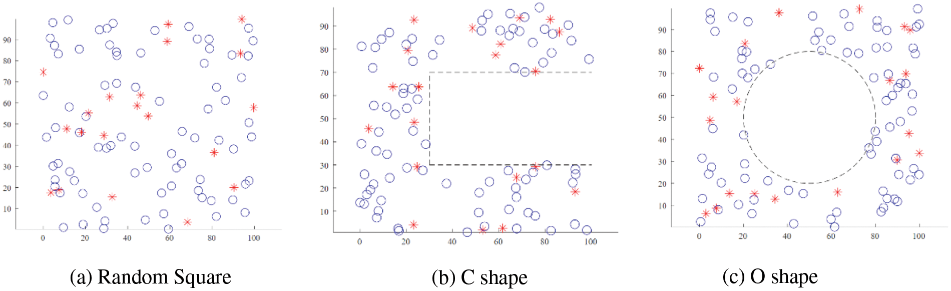
Figure 4: Different shape test networks showing anchor nodes and unknown nodes positions: (a) Random Square, (b) C shape, (c) O shape

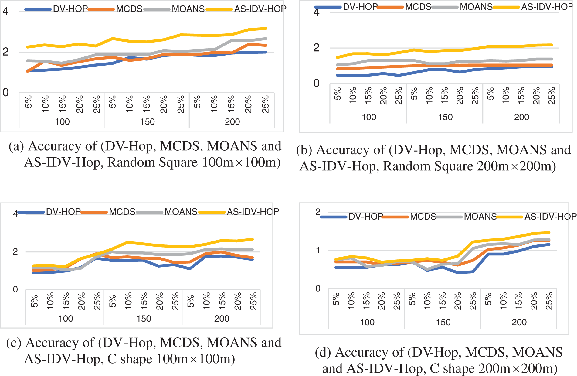
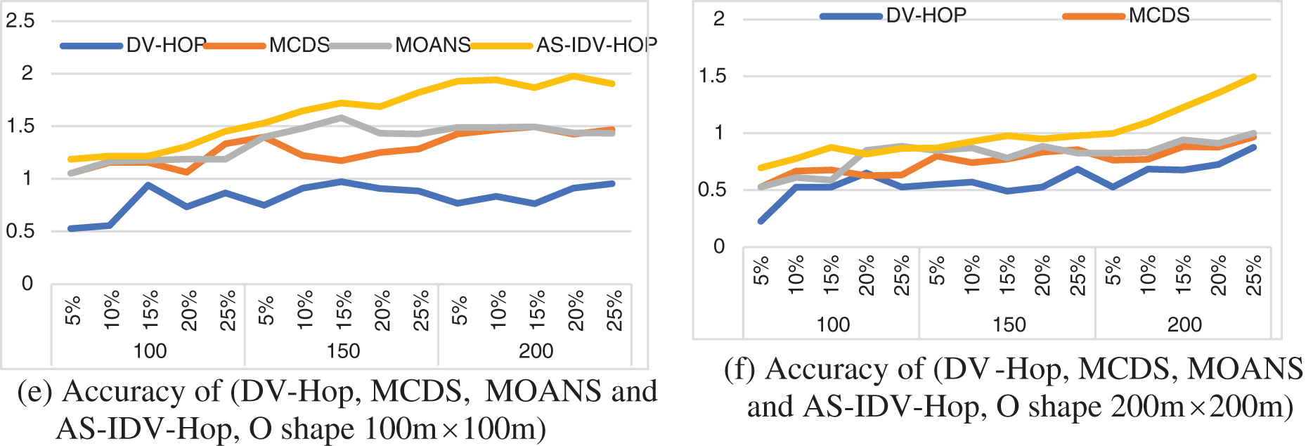
Figure 5: Localization accuracy graphs DV-Hop, MCDS, MOANS and AS-IDV-Hop: (a) Random Square 100 m × 100 m, (b) Random Square 200 m × 200 m, (c) C shape 100 m × 100 m, (d) C shape 200 m × 200 m, (e) O shape 100 m × 100 m, (f) O shape 200 m × 200 m

Fig. 6 shows the localization accuracy and variance of all algorithms. The proposed algorithm performs better if we decrease the ratio of anchor. Table 4 shows the localization accuracy of each algorithm with a different number of total sensor nodes. The results reveal notable trends in the performance of four localization algorithms across different anchor node ratios.

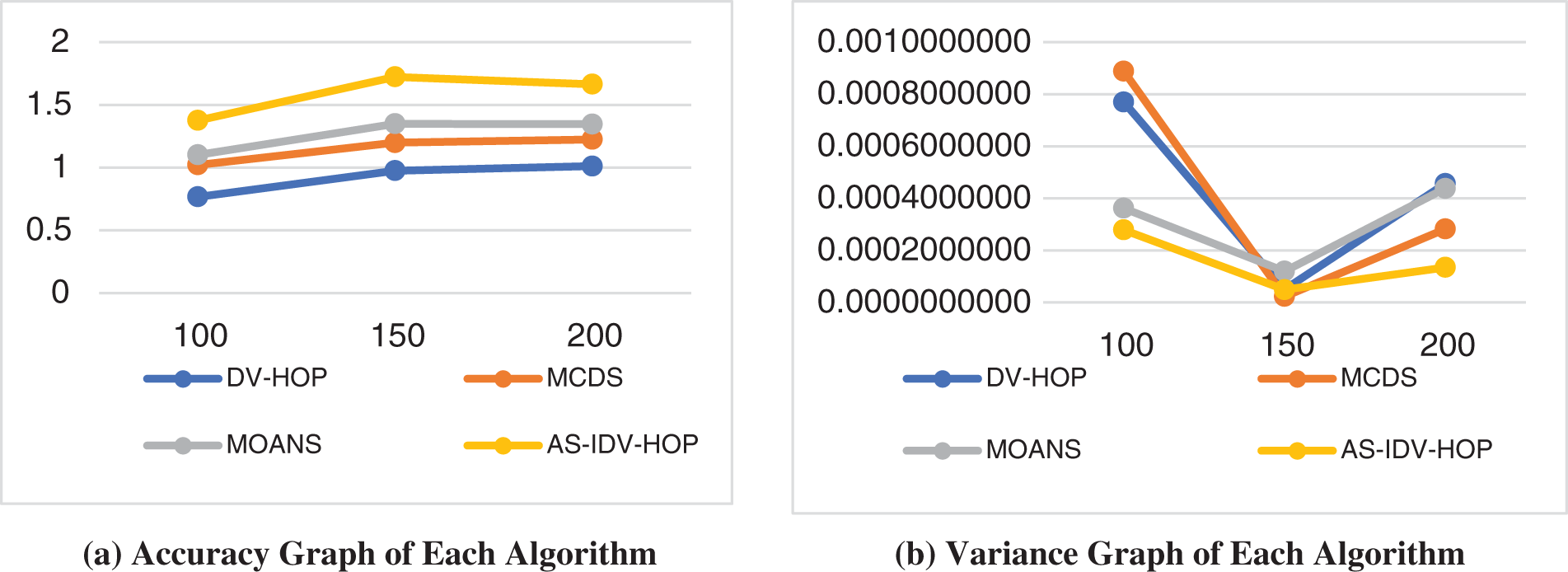
Figure 6: Localization accuracy graph and variance graph for each algorithm: (a) Accuracy graph, (b) variance graph

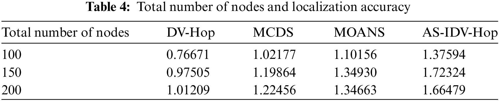
As the number of nodes ratio increases from 100 to 200, AS-IDV-Hop consistently outperforms the others at all anchor densities, indicating its superior ability to utilize anchor nodes effectively. Notably, while Niculescu et al. [7] and Kumar et al. [17] showed moderate and steady improvements, respectively, Rayavarapu et al. [9] exhibited a significant accuracy increase, particularly between 15% and 25% anchor ratios, suggesting it might require a higher density of anchors to optimize performance. The proposed AS-IDV-Hop algorithm not only achieves the highest accuracy values. It demonstrates the most significant improvement as sensor node density increases, reaching an accuracy of 1.37594, 1.72324, and 1.66479 at 100 m × 100 m and 200 m × 200 m. The mean accuracy of Niculescu et al. [7] is 0.91795, Kumar et al. [17] is 1.14832 and Rayavarapu et al. [9] is 1.26583 and the proposed AS-IDV-Hop is 1.58799. The variance is 0.01169, 0.00812, 0.01350, and 0.02311, respectively, and the standard deviations are 0.1080, 0.0901, 0.1162, and 0.1518, respectively.

So, it is proved that the improvement over traditional DV-Hop is 73.00%, MCDS-DV-Hop is 38.28%, and 25.44% over the MOANS-DV-Hop algorithm. This indicates that AS-IDV-Hop is particularly useful, making it suitable for applications requiring high localization accuracy.

5  Conclusion

Localization is needed for various applications, i.e., tracking of objects; localization techniques provide localization solutions but with many anchor nodes that increase the cost of the network and provide less accuracy. An important drawback in existing systems is the absence of a methodical strategy for choosing suitable anchor nodes and assistant anchor nodes for the localization process. Moreover, the average distance between hops is identified as a vibrant element that significantly affects the accuracy of localization. If there are any inaccuracies in this parameter, it could considerably reduce the effectiveness of the entire system. The proposed methodology tackles these problems by introducing a strong mechanism for strategically selecting anchor nodes and assistant anchor nodes in the localization process. Moreover, it includes a correction factor to address any insufficiencies in the calculation of the average hop distance between nodes. Our proposed technique aims to enhance the precision and effectiveness of localization in wireless sensor networks through implementation and validation. This offers a cost-efficient alternative when GPS infrastructure is not available. The proposed AS-IDV-Hop algorithm shows a notable improvement in accuracy over the other algorithms, the mean accuracy of Niculescu et al. [7] is 0.91795, Kumar et al. [17] is 1.14832 and Rayavarapu et al. [9] is 1.26583 and the proposed AS-IDV-Hop is 1.58799. The variance is 0.01169, 0.00812, 0.01350, and 0.02311, respectively, and the standard deviations are 0.1080, 0.0901, 0.1162, and 0.1518, respectively. So, it is proved that the improvement over traditional DV-Hop is 73.00%, MCDS-DV-Hop is 38.28%, and 25.44% over the MOANS-DV-Hop algorithm, respectively. This indicates that AS-IDV-Hop is particularly useful, making it a suitable choice for applications requiring high localization accuracy.

In the future, it would be advantageous to expand and refine the proposed approach to better accommodate evolving environmental conditions. Moreover, there is potential for research to delve into the creation of machine learning algorithms aimed at pinpointing adaptable anchor nodes, thus enhancing the system’s adaptability and efficiency. Exploring energy-saving strategies and investigating the integration of emerging technologies could also boost the development of Wireless Sensor Networks for localization purposes.

Acknowledgement: The authors extend their appreciation to the Department of Computer Science, Faculty of Computing, Universiti Teknologi Malaysia, for their institutional support, and to the Deanship of Research and Graduate Studies at King Khalid University for their financial support.

Funding Statement: This research was supported by the Deanship of Research and Graduate Studies at King Khalid University through a Large Research Project under grant number RGP.2/259/45.

Author Contributions: Muhammad Aamer Ejaz conceived the study, led the investigation, conducted experiments, and wrote the original draft. Kamalrulnizam Abu Bakar and Ismail Fauzi Bin Isnin assisted with data analysis and provided critical revisions. Babangida Isyaku and Taiseer Abdalla Elfadil Eisa provided additional research insights. Abdelzahir Abdelmaboud and Asma Abbas Hassan Elnour reviewed and approved the final manuscript. All authors reviewed the results and approved the final version of the manuscript.

Availability of Data and Materials: The data that support the findings of this study are available from the corresponding author, Muhammad Aamer Ejaz and Babangida Isyaku, upon reasonable request.

Ethics Approval: Not applicable.

Conflicts of Interest: The authors declare that they have no conflicts of interest to report regarding the present study.

References

1. P. Biswas, T. -C. Lian, T. -C. Wang, and Y. Ye, “Semidefinite programming based algorithms for sensor network localization,” ACM Trans. Sens. Netw., vol. 2, no. 2, pp. 188–220, 2006. doi: 10.1145/1149283.1149286. [Google Scholar] [CrossRef]

2. L. Gui, X. Zhang, Q. Ding, F. Shu, and A. Wei, “Reference anchor selection and global optimized solution for DV-Hop localization in wireless sensor networks,” Wirel. Pers. Commun., vol. 96, no. 4, pp. 5995–6005, 2017. doi: 10.1007/s11277-017-4459-x. [Google Scholar] [CrossRef]

3. A. Kaur, P. Kumar, and G. P. Gupta, “A new localization using single mobile anchor and mesh-based path planning models,” Wirel. Netw., vol. 25, no. 5, pp. 2919–2929, 2019. doi: 10.1007/s11276-019-02013-7. [Google Scholar] [CrossRef]

4. A. Mackey and P. Spachos, “LoRa-based localization system for emergency services in GPS-less environments,” in IEEE INFOCOM 2019-IEEE Conf. Comput. Commun. Work. (INFOCOM WKSHPS), 2019, pp. 939–944. doi: 10.1109/INFCOMW.2019.8845189. [Google Scholar] [CrossRef]

5. Y. Sun, X. Wang, J. Yu, and Y. Wang, “Heuristic localization algorithm with a novel error control mechanism for wireless sensor networks with few anchor nodes,” J. Sens., vol. 2018, pp. 1–16, 2018. doi: 10.1155/2018/5190543. [Google Scholar] [CrossRef]

6. U. Nazir, N. Shahid, M. A. Arshad, and S. H. Raza, “Classification of localization algorithms for wireless sensor network: A survey,” in ICOSST 2012-2012 Int. Conf. Open Source Syst. Technol. Proc., Aug. 2012, pp. 60–64. doi: 10.1109/ICOSST.2012.6472830. [Google Scholar] [CrossRef]

7. D. Niculescu and B. Nath, “DV based positioning in ad hoc networks,” Telecommun. Syst., vol. 22, no. 1–4, pp. 267–280, 2003. doi: 10.1023/A:1023403323460. [Google Scholar] [CrossRef]

8. Y. Cao and J. Xu, “DV-Hop-based localization algorithm using optimum anchor nodes subsets for wireless sensor network,” Ad Hoc Netw., vol. 139, 2023, Art. no. 103035. doi: 10.1016/j.adhoc.2022.103035. [Google Scholar] [CrossRef]

9. V. C. Rayavarapu and A. Mahapatro, “MOANS DV-Hop: An anchor node subset based localization algorithm for wireless sensor networks,” Ad Hoc Netw., vol. 152, Jan. 1, 2024, Art. no. 103323. doi: 10.1016/j.adhoc.2023.103323. [Google Scholar] [CrossRef]

10. Q. Zhao, Z. Xu, and L. Yang, “An improvement of DV-Hop localization algorithm based on cyclotomic method in wireless sensor networks,” Appl. Sci., vol. 13, no. 6, 2023, Art. no. 3597. doi: 10.3390/app13063597. [Google Scholar] [CrossRef]

11. Y. Cao, Y. Qian, and Z. Wang, “DV-Hop based localization algorithm using node negotiation and multiple communication radii for wireless sensor network,” Wirel. Netw., vol. 29, no. 8, pp. 3493–3513, 2023. doi: 10.1007/s11276-023-03417-2. [Google Scholar] [CrossRef]

12. F. Zeng, W. Li, and X. Guo, “An improved DV-Hop localization algorithm based on average hop and node distance optimization,” in Proc. 2018 2nd IEEE Adv. Inf. Manag. Commun. Electron. Autom. Control Conf. IMCEC 2018, vol. 11, pp. 1336–1339, 2018. doi: 10.1109/IMCEC.2018.8469655. [Google Scholar] [CrossRef]

13. B. Isyaku and K. B. A. Bakar, “Managing smart technologies with software-defined networks for routing and security challenges: A survey,” Comput. Syst. Sci. Eng., vol. 47, no. 2, pp. 1839–1879, 2023. doi: 10.32604/csse.2023.040456. [Google Scholar] [CrossRef]

14. P. S. Patel and J. R. Patel, “Localization algorithm for mobile sensor nodes using 3D space in wireless sensor network,” Int. J. Recent Innov. Trends Comput. Commun., vol. 2, no. 1, pp. 58–62, 2014. [Google Scholar]

15. D. Zhang, Z. Fang, Y. Wang, H. Sun, and J. Cao, “A new improved range free algorithm based on DV-Hop in wireless sensor network,” J. Commun., vol. 10, no. 8, pp. 589–595, 2015. doi: 10.12720/jcm.10.8.589-595. [Google Scholar] [CrossRef]

16. Y. Cao and Z. Wang, “Improved DV-hop localization algorithm based on dynamic anchor node set for wireless sensor networks,” IEEE Access, vol. 7, pp. 124876–124890, 2019. doi: 10.1109/ACCESS.2019.2938558. [Google Scholar] [CrossRef]

17. G. Kumar, M. K. Rai, R. Saha, and H. Kim, “An improved DV-Hop localization with minimum connected dominating set for mobile nodes in wireless sensor networks,” Int. J. Distrib. Sens. Netw., vol. 14, no. 1, 2018. doi: 10.1177/1550147718755636. [Google Scholar] [CrossRef]

18. Y. Zhang, S. Xiang, W. Fu, and D. Wei, “Improved normalized collinearity DV-Hop algorithm for node localization in wireless sensor network,” Int. J. Distrib. Sens. Netw., vol. 10, no. 7, 2014, Art. no. 436891. doi: 10.1155/2014/436891. [Google Scholar] [CrossRef]

19. R. Misra and C. Mandal, “A collaborative cover heuristic for ad hoc sensor networks,” IEEE Transactions on Parallel and Distributed Systems, vol. 21, no. 3, pp. 292–302, 2010. [Google Scholar]

20. S. J. Bhat and S. K. Venkata, “An optimization based localization with area minimization for heterogeneous wireless sensor networks in anisotropic fields,” Comput. Netw., vol. 179, May 2020, Art. no. 107371. doi: 10.1016/j.comnet.2020.107371. [Google Scholar] [CrossRef]

21. Z. Guo, L. Min, H. Li, and W. Wu, “Improved DV-Hop localization algorithm based on RSSI value and hop correction,” presented at the 6th China Conf. Wirel. Sens. Netw. (CWSN), Huangshan, China, Springer, Oct. 25–27, 2012, vol. 6, pp. 97–102. [Google Scholar]

22. T. Kunz and B. Tatham, “Localization in wireless sensor networks and anchor placement,” J. Sens. Actuator Netw., vol. 1, no. 1, pp. 36–58, 2012. doi: 10.3390/jsan1010036. [Google Scholar] [CrossRef]

23. H. Chenji and R. Stoleru, “Mobile sensor network localization in harsh environments,” in Int. Conf. Distrib. Comput. Sens. Syst., Springer, 2010, pp. 244–257. [Google Scholar]

24. P. Raguraman, M. Ramasundaram, and V. Balakrishnan, “Localization in wireless sensor networks: A dimension based pruning approach in 3D environments,” Appl. Soft Comput., vol. 68, no. 4, pp. 219–232, 2018. doi: 10.1016/j.asoc.2018.03.039. [Google Scholar] [CrossRef]

25. J. Li, J. Zhang, and X. Liu, “A weighted DV-Hop localization scheme for wireless sensor networks,” in Int. Conf. Scalable Comput. Commun. Eighth Int. Conf. Embed. Comput., IEEE, 2009, pp. 269–272. [Google Scholar]

26. H. Sun, H. Li, Z. Meng, and D. Wang, “An improvement of DV-Hop localization algorithm based on improved adaptive genetic algorithm for wireless sensor networks,” Wirel. Pers. Commun., vol. 130, no. 3, pp. 2149–2173, 2023. doi: 10.1007/s11277-023-10376-6. [Google Scholar] [CrossRef]

27. P. Wang, X. Wang, W. Li, X. Fan, and D. Zhao, “DV-Hop localization based on distance estimation using multinode and hop loss in WSNs,” Mar. 7, 2024, arXiv:2403.04365. [Google Scholar]

28. W. Xue, W. Qiu, X. Hua, and K. Yu, “Improved Wi-Fi RSSI measurement for indoor localization,” IEEE Sens. J., vol. 17, no. 7, pp. 2224–2230, 2017. doi: 10.1109/JSEN.2017.2660522. [Google Scholar] [CrossRef]

29. N. Li, L. Liu, D. Zou, and X. Liu, “Node Localization algorithm for irregular regions based on particle swarm optimization algorithm and reliable anchor node pairs,” IEEE Access, vol. 12, pp. 37470–37482, 2024. doi: 10.1109/ACCESS.2024.3374518. [Google Scholar] [CrossRef]

30. S. Phoemphon, C. So-In, and N. Leelathakul, “A hybrid localization model using node segmentation and improved particle swarm optimization with obstacle-awareness for wireless sensor networks,” Expert Syst. Appl., vol. 143, 2020, Art. no. 113044. doi: 10.1016/j.eswa.2019.113044. [Google Scholar] [CrossRef]

31. D. Han, Y. Yu, K. C. Li, and R. F. de Mello, “Enhancing the sensor node localization algorithm based on improved DV-Hop and DE algorithms in wireless sensor networks,” Sensors, vol. 20, no. 2, 2020, Art. no. 343. doi: 10.3390/s20020343. [Google Scholar] [PubMed] [CrossRef]

32. A. Kaur, P. Kumar, and G. P. Gupta, “A weighted centroid localization algorithm for randomly deployed wireless sensor networks,” J. King Saud Univ. Comput. Inf. Sci., vol. 31, no. 1, pp. 82–91, 2019. doi: 10.1016/j.jksuci.2017.01.007. [Google Scholar] [CrossRef]

33. V. Kanwar and A. Kumar, “DV-Hop based localization methods for additionally deployed nodes in wireless sensor network using genetic algorithm,” J. Ambient Intell. Humaniz. Comput., vol. 11, no. 11, pp. 5513–5531, Nov. 2020. doi: 10.1007/s12652-020-01907-1. [Google Scholar] [CrossRef]

34. V. Kanwar, “Efficient node localization on sensor internet of things networks using deep learning and virtual node simulation,” Electronics, vol. 13, no. 8, pp. 1–16, 2024. [Google Scholar]

35. F. Liu and G. Feng, “Research on location feedback based DV-Hop localization algorithm,” in Key Engineering Materials, Trans Tech Publications, Ltd., 2014, vol. 621, pp. 699–706. doi: 10.4028/www.scientific.net/KEM.621.699. [Google Scholar] [CrossRef]

36. M. Rai, S. Verma, and S. Tapaswi, “A power aware minimum connected dominating set for wireless sensor networks,” J. Netw., vol. 4, no. 6, pp. 511–519, 2009. doi: 10.4304/jnw.4.6.511-519. [Google Scholar] [CrossRef]

37. D. Wang, K. B. A. Bakar, and B. Isyaku, “A survey on IoT task offloading decisions in multi-access edge computing: A decision content perspective,” Qubahan Acad. J., vol. 3, no. 4, pp. 422–436, 2023. doi: 10.58429/qaj.v3n4a220. [Google Scholar] [CrossRef]

38. O. Cheikhrouhou, G. M. Bhatti, and R. Alroobaea, “A hybrid DV-Hop algorithm using RSSI for localization in large-scale wireless sensor networks,” Sensors, vol. 18, no. 5, 2018, Art. no. 1469. doi: 10.3390/s18051469. [Google Scholar] [PubMed] [CrossRef]

39. C. Phillips, D. Sicker, and D. Grunwald, “A survey of wireless path loss prediction and coverage mapping methods,” IEEE Commun. Surv. Tutor., vol. 15, no. 1, pp. 255–270, 2013. doi: 10.1109/SURV.2012.022412.00172. [Google Scholar] [CrossRef]

40. F. Zafari, I. Papapanagiotou, and K. Christidis, “Microlocation for internet-of-things-equipped smart buildings,” IEEE Internet Things J., vol. 3, no. 1, pp. 96–112, 2016. doi: 10.1109/JIOT.2015.2442956. [Google Scholar] [CrossRef]

41. L. Sun and T. Chen, “Difference DV_distance localization algorithm using correction coefficients of unknown nodes,” Sensors, vol. 18, no. 9, 2018, Art. no. 2860. doi: 10.3390/s18092860. [Google Scholar] [PubMed] [CrossRef]

42. S. Afzal and H. Beigy, “A localization algorithm for large scale mobile wireless sensor networks: A learning approach,” J. Supercomput., vol. 69, no. 1, pp. 98–120, 2014. doi: 10.1007/s11227-014-1129-6. [Google Scholar] [CrossRef]

43. D. Niculescu and B. Nath, “Ad hoc positioning system (APS) presented in IEEE INFOCOM 2003,” Twenty-Second Annu. Joint Conf. IEEE Comput. Commun. Societies, vol. 3, pp. 1734–1743, Mar. 30, 2003. [Google Scholar]

44. A. K. Paul, Y. Li, and T. Sato, “A distributed range-free sensor localization with friendly anchor selection strategy in anisotropic wireless sensor networks,” J. Japan Society Simul. Technol., vol. 4, no. 3, pp. 96–106, Aug. 2012. [Google Scholar]