HQNN-SFOP: Hybrid Quantum Neural Networks with Signal Feature Overlay Projection for Drone Detection Using Radar Return Signals—A Simulation

1  Introduction

Signal detection extracts the relevant parameters of the signals containing interference and noise received at the receiving end using statistical theory, probability theory, and other methods to determine whether the target signal exists. Signal detection can accurately and effectively identify and distinguish target signals, which is of great significance in enhancing the detection capability in complex environments, improving the anti-interference capability of the system, and providing auxiliary decision support. Radar return signal detection is an important applied research direction.

As a new type of aerial vehicle, drones are playing an increasing role in applications such as courier transportation [1,2], emergency medical care [3], healthcare [4], precision agriculture [5], and forestry protection [6]. The use of drones brings convenience but is also accompanied by security and privacy, air traffic, noise pollution, misuse in illegal areas, and other problems, so it is necessary to use technical means to detect and identify them, and to carry out monitoring, scheduling, and management of drones.

With signal detection rapidly entering the intelligent analysis stage, intelligent signal detection techniques based on machine learning are playing an increasingly important role. Radar sensors have the advantages of working efficiently and stably in complex environments and having a wide detection range. Extracting the spectrogram of radar return signals using short-time Fourier (STFT) and then applying machine learning algorithms to learn the spectrogram is an important drone detection method [7–9]. However, this method has the problem of high dimensionality of image features, which makes the input data processing of the machine learning model huge, and there are a large number of redundant features, and the noise can easily interfere with the model learning [10]. Therefore, we propose to extract the time-domain statistical features in the radar return signals that are related to drone detection for analysis and processing, and when the extracted time-domain statistical features have enough information about drone detection, the accuracy of detection can be effectively improved while reducing the feature dimensions, which is proved in Experiment 4.5.

The large reduction in data dimensions can lead to low accuracy of classical machine learning models in this task. Quantum computation is executed in Hilbert space and realized by quantum entanglement, superposition, and other properties [11], which have advantages unmatched by classical vector space [12,13], and these advantages have also been proved by experiments [14]. As quantum computing enters the NISQ era [15], quantum intelligence work based on quantum computing technology is gradually carried out, and many scholars have demonstrated that various types of classical machine learning algorithms after quantum optimization have been improved in terms of performance and robustness compared with the original classical machine learning algorithms [16–18].

Hybrid quantum neural networks use quantum mechanics to optimize the classical machine learning process, and use classical neural network architecture to drive parameterized quantum circuits to learn specified tasks, achieving high accuracy and efficiency [19,20]. Therefore, we introduce a hybrid quantum neural network and apply the advantage of quantum-specific superposition in Hilbert space to obtain the inline relationship of low-latitude signal features, to improve the accuracy of detecting drones using radar return signals as well as enhance the migration generalization ability, which is verified in Experiment 4.5 and Experiment 4.6.

Machine learning requires a large amount of data and therefore simulated data is needed to emulate real data scenarios. We chose to use the MM model [21,22] to simulate the generation of radar return signals from drones. The MM model is used to simulate the radar return signals from the propeller blades of the aircraft, so by choosing the appropriate parameters and introducing the real parameters of the drone, it can be used to simulate the radar return signals from the propeller blades of the drone. In addition, the MM model can simulate different signal-to-noise ratio conditions, making the data more capable of imitating reality [23]. The researcher migrated the model generated by training on the MM model simulation data to a real-world drone dataset collected using radar, which could achieve a peak performance of 0.700 in F1-score, thus demonstrating the feasibility of machine learning for drone detection on simulated samples generated using the MM model to aid in real-world drone detection research [24]. Based on the MM model, on the one hand, the parameters of five real commercial drones were used to generate the dataset, and on the other hand, to adapt to the uncertainty in the real environment, random drones parameters were also used to generate the dataset for comparative analysis.

Overall, this paper proposes a new Hybrid Quantum Neural Network with Signal Feature Overlay Projection (HQNN-SFOP) for drone detection using radar return signals and experiments on the simulated datasets. The contributions of this paper are as follows:

1. This study proposes a signal time-domain statistical feature extraction method, which extends the field of view for extracting the features of radar return signals from drones and provides a new analytical perspective and processing strategy in this field.

2. We apply a hybrid quantum neural network to the detection of radar return signals from drones and successfully introduce the superposition property of quantum computing into the field of signal processing, which realizes the quantum intelligent processing of radar signals from drones.

3. We propose HQNN-SFOP, a signal detection method combining the signal time-domain statistical features and the hybrid quantum neural networks, which opens up a novel method different from time-frequency-domain features combined with classical CNN for drone detection using radar return signals.

4. Compared with traditional methods, HQNN-SFOP not only has smaller feature dimensions, but also exhibits higher accuracy and migration generalization ability, which significantly improves the efficiency and performance of detecting drones using radar return signals, and provides valuable experience and technical accumulation in the field of signal processing and machine learning.

The paper is structured as follows:

Section 2 is the background, which introduces the research status of drone detection and signal feature extraction. Section 3 is the methods, which introduces the overall architecture and details the various aspects of the architecture, including the generation of radar return signals from drones, statistical feature extraction in the time domain of the signal, and Hybrid Quantum Neural Networks with Signal Feature Overlay Projection. Section 4 is experiments and results, describes the datasets used for the experiments, as well as the baseline, data preprocessing and feature selection, and the results of the experiments, including a comparison of the results with the classical machine learning algorithms, a comparison of the migration generalization capabilities and the ablation study. Section 5 proceeds to summarize the paper and discusses future research directions.

2  Background

2.1 Drone Detection

Existing sensors for drone surveillance include acoustic sensors, optical sensors, and radar sensors. Acoustic sensors utilize microphones to capture the acoustic signals from the drone and then use acoustic processing to detect the drone [25,26]. However, acoustic sensors have a small operating range, some with a surveillance distance of only 200 m, and they cannot work in bad weather conditions such as rain or snow, and are easily affected by noise in the environment. Optical sensors utilize cameras to track drones and process image and video data for drone detection [27,28]. Optical sensors are limited by the camera’s viewing angle and range of capture, and nighttime, extreme weather conditions, and the presence of obstacles can affect the sensor’s ability to capture. Radar is an important device for drone detection because of its adaptability to weather and lighting conditions, its wide coverage, and its ability to monitor in cluttered environments [7].

There have been researchers using classical machine learning methods combined with radar return signals to carry out drone detection tasks, using machine learning algorithms including SVM [8], DecisionTree [29], CNN [28,30,31], and so on. Most of these methods use Short Time Fourier (STFT) to extract the spectral image dataset and machine learning algorithms then detect and classify the image data [7,23], CNNs can achieve optimal performance [9]. However, the method based on image recognition to detect radar return signals from drones suffers from the problem of high dimensionality of image features. The common datasets for existing image recognition techniques have a minimum image dimension of 28 × 28 [32,33], and the spectrogram feature dimensions of the radar return signals from drones will only be higher, for example, the size of the spectrogram in the paper [24] is 512 × 4, the high-latitude features make the amount of input data processing for machine learning models very large, on the other hand, many of these image features are irrelevant to signal detection, but will instead bring interference to model learning [10]. Therefore, there is a need to find low-latitude features that are sufficient to characterize the detection of radar return signals from drones.

2.2 Signal Feature Extraction

In signal processing, raw signals often have very complex characteristics and structures, which may be very difficult to analyze and process directly. Signal feature extraction can convert the original signal data into statistical quantities or other forms of information that can reflect the characteristics of the data, and the methods include time-domain extraction, frequency-domain extraction, and time-frequency domain extraction. Time domain features are used to extract the statistical characteristics of the signal on the time axis, such as the period of the signal, waveform, etc., which can reflect the fluctuation and transformation of the signal in time. Signal frequency domain feature extraction extracts the spectral information of the signal by frequency, including the amplitude and phase of different frequencies. Time-frequency domain feature extraction combines the time and frequency domains to show the characteristics of the signal in the time and frequency domains at the same time, in which the short-time Fourier transform is used more often to generate spectral maps [34]. Different feature extraction methods need to be selected according to different application scenarios.

Compared with the features extracted from frequency and time-frequency domains, time-domain features are easy to extract. In addition, Compared with image recognition, there are several advantages of time-domain statistical features, firstly, it can better capture the essential properties of the signal, discover the salient laws and statistical characteristics of the signal, and improve the accuracy of analysis; secondly, compared with high-latitude image features, it can accurately focus on the subtle characteristics that are more relevant to signal detection, downsize the signal, reduce the amount of data processing of the model, simplify the processing, and improve the analysis efficiency; thirdly, the extraction of signal time domain statistical features can obtain the stable and invariant features of the signal, and has strong robustness to noise and other interference factors. The advantages of time-domain statistical feature extraction, such as enhanced accuracy, improved analysis efficiency, and high robustness, make it have a wide range of application prospects and potentials in the field of signal processing.

Therefore, we consider extracting time-domain statistical features of the signal, which are selected to have a small feature set size, high accuracy, and stronger stability when there is enough information to distinguish the drone from the noise case. The time-domain feature selection process is described in Experiment 4.4, and the time-domain feature extraction process is described in Section 3.3.

3  Methods

In this section, we first introduce the overall architecture of HQNN-SFOP and show the functions of each link in the framework by using a drone as an example. The subsequent subsections describe in detail the implementation methods of each link, respectively.

3.1 Structure

We use the hybrid quantum neural networks with signal feature overlay projection (HQNN-SFOP) to detect the simulated radar return signals generated by real drone parameters, and the links include the generation of radar return signals from drones, signal time-domain statistical feature extraction, and the detection by the hybrid quantum neural networks with signal feature overlay projection (Fig. 1). Next, we take the drone Parrot Disco as an example to show the functions of each link. The remaining four drones, DJI Mavic Air 2, DJI Mavic Mini, DJI Matrice 300 RTK, and DJI Phantom 4, are handled similarly.

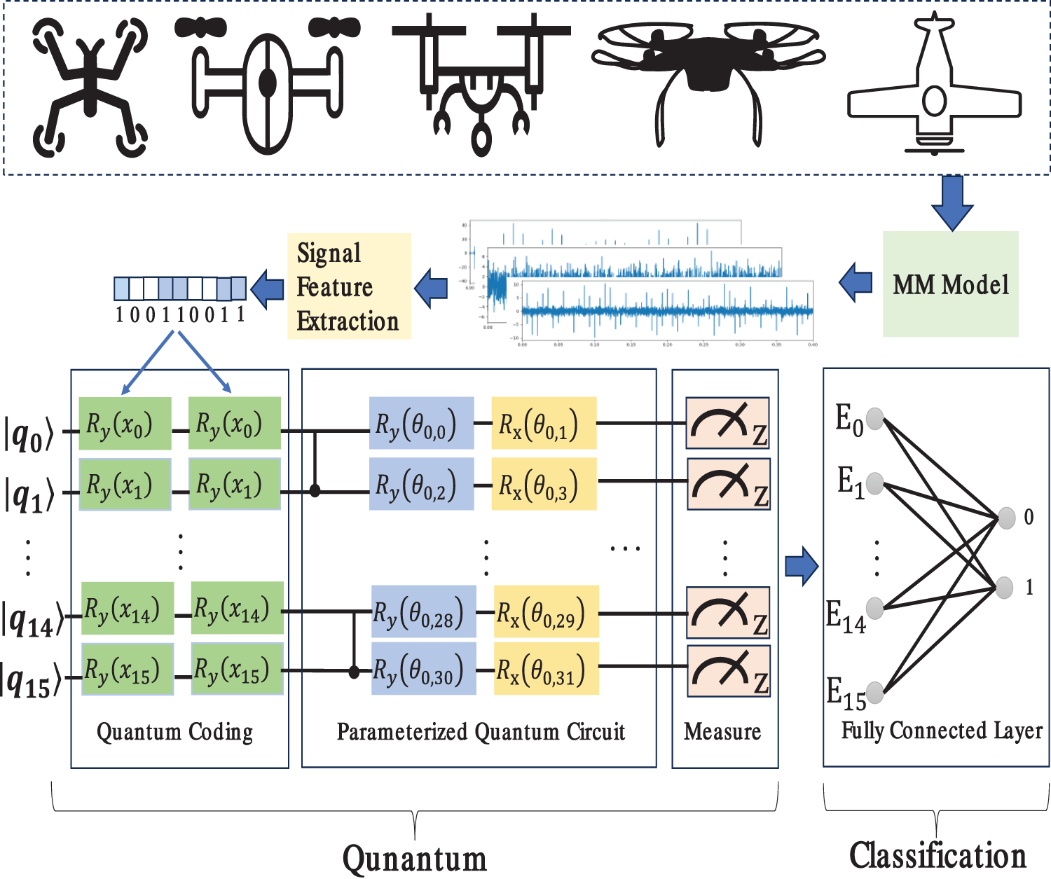
Figure 1: General structure

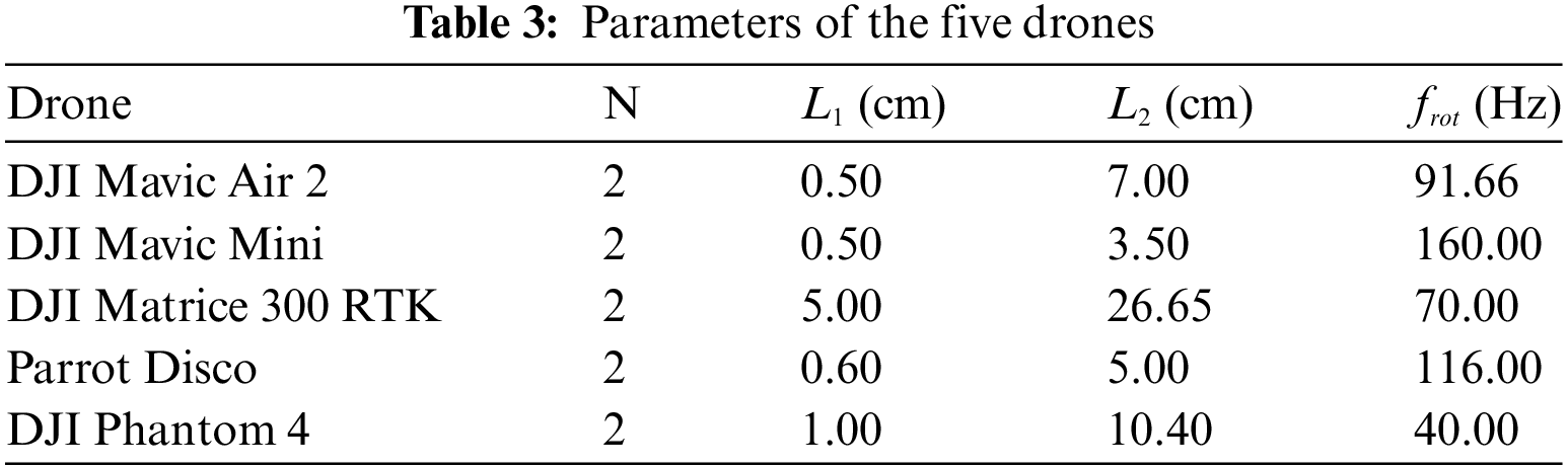
Parrot Disco is a drone used in various industries such as mapping, exploration, and environmental protection. It has 2 blades, the distance between the root of the blade and the center of rotation is 0.6 cm, the distance between the tip of the blade and the center of rotation is 5 cm, and the rotational frequency of the blade is 116 Hz.

Inputting these parameters of the Parrot Disco into the MM model allows for the generation of radar return signals that simulate the propeller blades of the drone. In addition, the model can add noise to the signal and also generate a noisy signal. Fig. 2 gives an example of the generation of a radar signal reflected from the drone Parrot Disco at an SNR of 10 dB. Fig. 3 gives an example of the noise signal.

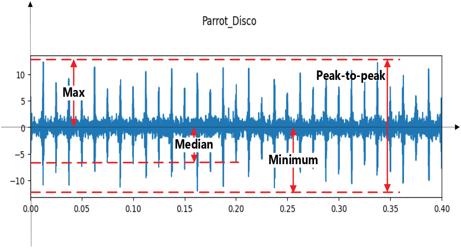
Figure 2: Real-valued portion of a radar signal reflected from the drone Parrot Disco with an SNR of 10 dB. The red line identifies some of the time-domain statistical features

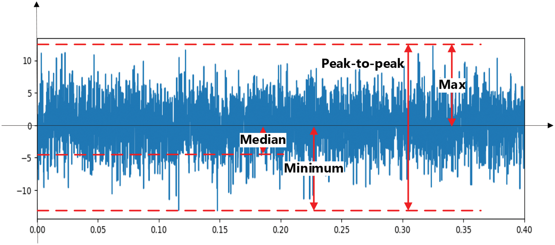
Figure 3: Real-valued portion of noise’s time series

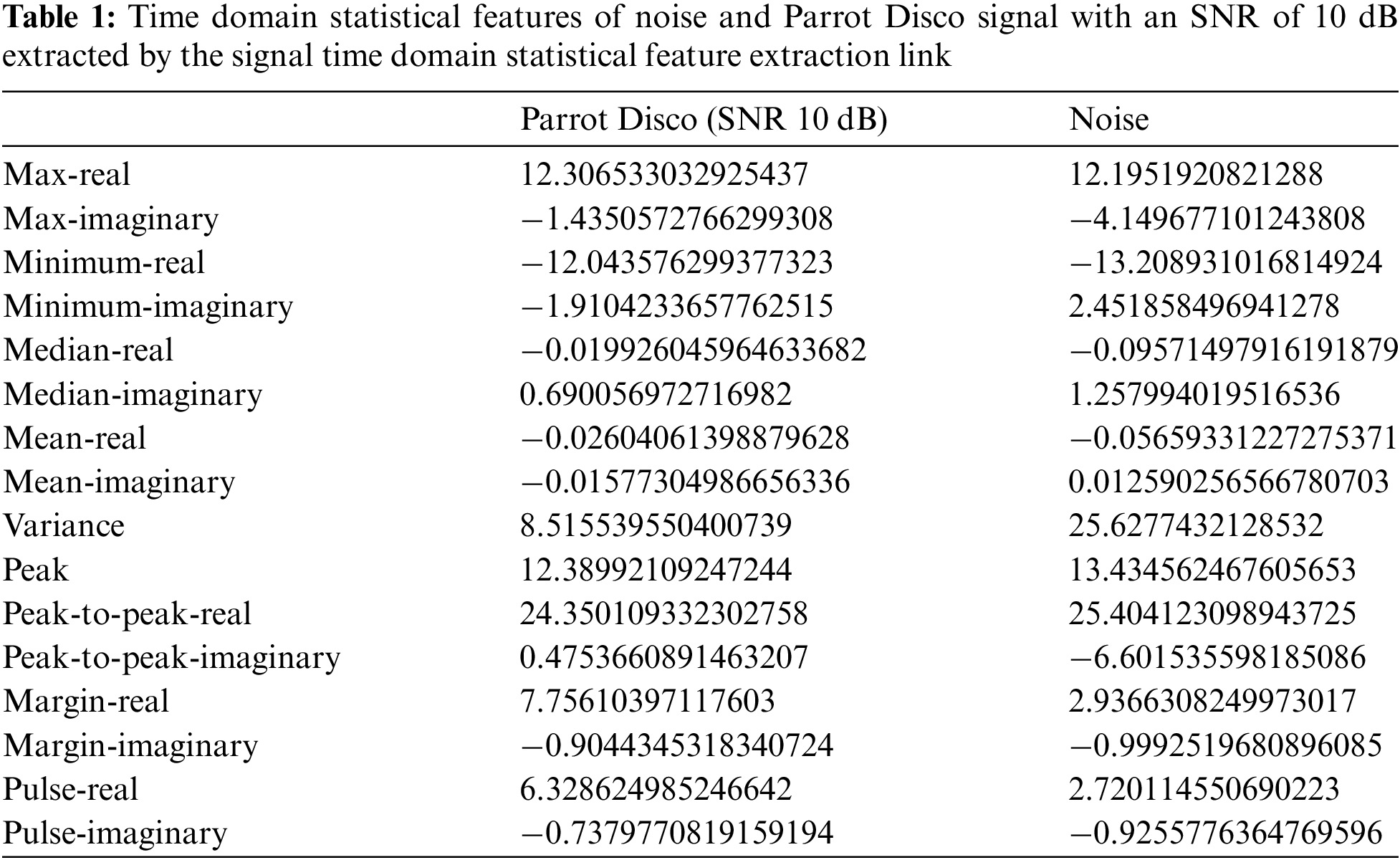
The signal time domain statistical feature extraction is performed on the radar return signal from drones and noise signals. Comparing Figs. 2 and 3, we can see that the drone signal and noise have different time domain statistical features such as maximum value, minimum value, median, peak-to-peak value, and so on. In terms of other subtle features such as mean, variance, peak, margin factor, impulse factor, and other subtle features that are not directly observable by the naked eye or image recognition, as well as the inline relationship of these subtle features, the drone and noise have even more significant differences. Therefore, these extracted statistical features in the time domain can be used as the object of HQNN-SFOP learning to detect drones and noise. For the time-domain statistical features extracted from the real-valued portion and imaginary portion of the signal, we obtain a total of 16-dimensional features as in Table 1, which are used for the subsequent learning of the HQNN-SFOP model.

The extracted time-domain statistical features are encoded from classical data into quantum states and input into the HQNN-SFOP model, where the signal feature superposition projection amplifies the subtle features of the quantum state signal eigenvectors, and the hybrid quantum neural networks model learns the inline relationships of these features to detect drones and noise.

We explore the potential of drone detection tasks through quantum computing. On the one hand, it expands new application areas for quantum computing and explores its advantages in the field of signal analysis; on the other hand, it also explores feasible directions for the iterative technological evolution of signal intelligence analysis and lays the foundation for the application of future disruptive computing technologies. In the following, we will introduce each link in the process in detail.

3.2 Generation of Radar Return Signals for Drones

To compare the results, we use the previous method [24] to generate drone signal and noise datasets by applying the MM model. The MM model combines the application of electromagnetic wave theory, and by inputting different parameters to it, it can simulate the radar return signals of different aircraft propeller blades, which are defined as follows:

Ψ(t)=Arej(2πfct−4πλ(R+Vradt))∑n=0N−1(α+βcos⁡(Ωn))e−jL1+L22γnsinc(L2−L12γn)(1)

where

α=sin⁡(|θ|+Φp)+sin⁡(|θ|−Φp)

β=sign(θ)(sin⁡(|θ|+Φp)−sin⁡(|θ|−Φp))

Ωn=2π(frott+nN)

γn=4πλcos⁡(θ)sin⁡(Ωn)

The parameters used in the MM model are explained in Table 2. These parameters are categorized by function into radar characterization parameters, aircraft characterization parameters, and aircraft-radar positional relationship characterization parameters. Configuring the two radar characteristic parameters fc and λ identifies the particular radar that one wishes to simulate. By configuring N, L1, L2, and frot these aircraft characteristic parameters can determine the aircraft blade characteristics and thus specify the aircraft type. Configuring θ, Φp, R, and Vrad then specifies the aircraft position.

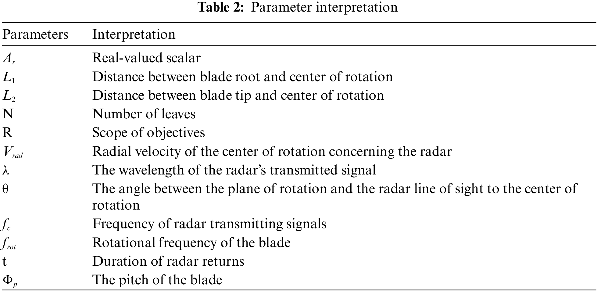
The simulated radar emission signal is an X-band signal with an emission frequency fc of 10 GHz and a wavelength λ of 3 cm. Five real commercial drones, DJI Mavic Air 2, DJI Mavic Mini, DJI Matrice 300 RTK, DJI Phantom 4, and Parrot Disco, are simulated here to generate samples, each of which is generated by the parameters of one of the five drones were simulated to generate the samples. The parameters of the five drones are shown in Table 3.

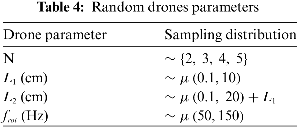
To accommodate uncertainty in real-world environments, a set of randomized drones datasets were generated for comparative analysis using the parameters in Table 4. The number of blades N in Table 4 is any integer between 2 and 5, while L1, L2, and frot are random values within a specific range, which are reasonably filtered to accommodate a variety of new and ever-innovating drones. In addition, the value of L2 is an increase from L1 to ensure that the parameters are consistent with the characteristic that the distance between the tip of the blade and the center of rotation of a real drone is greater than the distance between the root of the blade and the center of rotation.

The parameters θ, Φp, and Vrad are configured in Table 5.

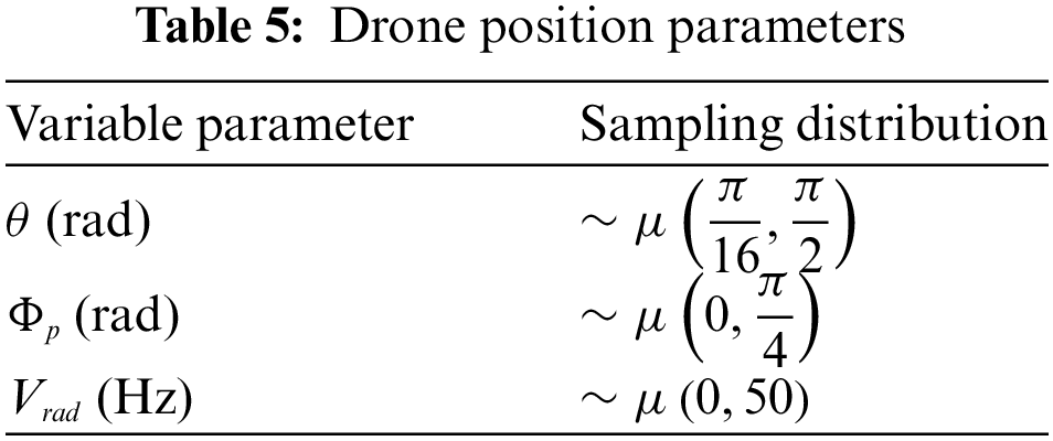
In combination with the real-valued scalar Ar, noise can be introduced in the signal. The noise is derived from the single-pulse signal-to-noise ratio, and the equation is defined as follows:

SNR=10log10(Ar2δn2)(2)

The noise δn can be solved for according to the above equation, and the noise added to the signal is obtained by sampling in υ∼N(0, δn).

3.3 Extraction of Statistical Features in the Time Domain of the Signal

Our feature extraction method is different from other methods, which use the Fourier transform to obtain spectrograms and then learn image features to detect them by classical machine learning methods. For the radar signal generated by the MM model, we extract the time-domain statistical features with strong relevance to drone detection, including the maximum, minimum, median, mean, variance, peak, peak-to-peak, margin factor, impulse factor, etc., which are used to describe the statistical properties of the signal. HQNN-SFOP is used to learn the inline relationship of the 16-dimensional features to detect the signals. These features are defined and described as follows:

Max: Maximum value of the sampling result of each sampling point of the signal.

SC1=max(xi)(3)

Minimum: Minimum value of the sampling result of each sampling point of the signal.

SC2=min(xi)(4)

Median: The sampling value in the signal is in the middle of each sampling point.

SC3={xn+12n is an odd numberxn2+xn2+12n is an even number(5)

Mean: Expectation, is the average value of each sample of the signal.

SC4=1n∑i=0n−1xi(6)

Variance: The mean of the squares of the difference between the sampled values and the average value of the signal, which reflects the degree of dispersion between the data.

SC5=1n∑i=0n−1(xi−SC4)2(7)

Peak: Maximum value of absolute value of each sample of signal.

SC6=max(|SC1|, |SC2|)(8)

Peak-to-peak: Difference between the maximum and minimum of the signal, describes the transform range of the signal.

SC7=SC1−SC2(9)

Margin: The ratio of the maximum value of the signal to the square of the square root of the expectation of the sampling result, which describes the transform margin of the signal.

SC8=SC1(1n∑i=0n−1|xi|)2(10)

Pulse: The ratio of the maximum value of the signal to the expected absolute value of the sampling result, which describes the pulse characteristic of the signal.

SC9=SC11n∑i=0n−1|xi|(11)

Due to the characteristics of the signal itself, Max, Minimum, Median, Mean, Peak-to-peak, Margin, and Pulse include real and imaginary values, thus forming 16-dimensional features. We analyze the correlation between these features and the labels through the feature selection of Experiment 4.4, and obtained the 16-dimensional feature selection scheme.

Compared with image detection, this method of extracting the statistical features of the signal in the time domain and then detecting them can more accurately obtain the subtle features of the signal, reduce the degree of redundancy of the feature data, and improve the detection ability of the signal processing, as well as effectively reduce the complexity of the HQNN-SFOP model, and improve the efficiency of the training and stability, which is effectively demonstrated in the later Experiment 4.5 and Experiment 4.6.

3.4 Hybrid Quantum Neural Networks with Signal Feature Overlay Projection

3.4.1 Signal Feature Overlay Projection

In classical signal processing, the analysis of signals is often limited by the quality of signal features in the sample set. Relevant studies have shown that in Hilbert space, quantum has a unique superposition recognition ability for information [35], and the use of this advantage can improve the expression ability of a quantum machine learning model [36]. We creatively apply this capability of quantum information in the field of signal processing to overlap the feature vectors of radar return signals from drones to amplify the subtle features of the processed objects and to enhance the representation of the feature vectors to the radar return signals.

Suppose |si⟩=(si0, si1,…,si(n−1))T is the radar return feature vector in quantum Hilbert space. The signal feature overlap projection formula for this vector is as follows:

Si=|si⟩|si⟩(12)

Signal feature overlap projection in quantum circuits is manifested by the fact that signal feature vectors are introduced into quantum bits more than once, and these quantum bits are not only affected by the previous quantum bit but also reintroduced into the input signal feature vectors each time, thus realizing the overlap operation on the signal feature vectors (e.g., Fig. 1).

Interpreted geometrically, the classification of a quantum classifier in Hilbert space is related to its layer in the Bloch sphere. The signal feature superposition projection operation corresponds to a unitary rotation, a rotation of quantum bits, which expands the single layer of feature data in the Bloch sphere into more layers [35], thus amplifying the subtle features of the signal and facilitating the learning of the quantum classifier. The quantum space sample set after signal feature overlap projection, compared to the sample set before overlap projection, can effectively improve the detection performance in the next stage of hybrid quantum learning training, as verified in Section 4.7.2.

3.4.2 Hybrid Quantum Neural Networks

The HQNN-SFOP in our study fully utilizes the advantages of quantum computing and consists of a hybrid of quantum feature learning module and classical optimization module (e.g., Fig. 1). The quantum feature learning module contains a quantum coding layer, a parameterized quantum circuits layer, and a quantum circuits measurement layer, which are used for data quantization processing and parameter learning of the sample set. The classical optimization module drives the quantum feature learning module to perform iterative optimization through the gradient descent algorithm so that the prediction results of the whole hybrid networks gradually approach the labeling results of the sample dataset.

Quantum Coding Layer

The quantum coding layer encodes classical data into quantum states for subsequent quantum manipulation and processing. We choose rotational coding for quantum coding and overlap projection of signal features on the quantum Hilbert space data of the samples. Rotational coding is a coding method for simple data sets. It introduces rotational operations to enrich the quantum representation of the data, which makes the data have more complex and rich states in the quantum space, and can more accurately represent and process data sets with complex structures or patterns with more expressive power and flexibility. The encoding of rotational encoding is a quantum bit-based embedding that encodes each feature s→i of the vector sij into the angle of rotation of the quantum bit through the Pauli rotation (σx, σy, σz), respectively, to obtain the data features, corresponding to the quantum state |sij⟩=cos⁡sij|0⟩+sin⁡sij|1⟩ form.

We use rotational coding in the quantum coding layer with overlap projection of signal features, which can extend the layers of feature data in the Bloch sphere and amplify the subtle features of the signal, effectively improving the detection performance of the hybrid quantum neural networks up to about 0.01 to 0.03 (Experiment 4.7.2), thus enhancing the model’s ability to represent the features in the radar return data of drones.

Parameterized Quantum Circuits Layer

The parameterized quantum circuits layer is responsible for processing quantum states, which can adjust the parameters of the quantum circuits according to the task requirements, simulate the data relations within the quantum states, extract the effective quantum features, and approximate the objective function within the allowable error range, and its function is similar to the hidden layer with significant expressive ability in the classical neural networks.

The configurable part of the parameterized quantum circuits layer includes the topology of the cell layer and its stacking times (i.e., the number of cell layers). The topology of the cell layer is composed of different selections and layouts of quantum gates with and without parameters. Quantum gates with parameters include Ry(θ), Rx(θ), etc., and quantum gates without parameters include CNOT. Rx(θ) means rotating the quantum state around the X-axis in Hilbert space, and Ry(θ) means rotating around the Y-axis.

The parameterized quantum circuits we designed are shown in Fig. 4, where the number of cell layers of the quantum circuits is 10 and the number of quantum bits is 16, mapping 16 features to 16 quantum bits, respectively. The use of the CNOT gate between each pair of quantum bits ensures that the quantum-encoded data realizes quantum state entanglement in Hilbert space. The entire quantum circuits consist of Ry(θ), Rx(θ) gates, and the role of parameter θ in the quantum circuits is similar to the weight in classical neural networks. In the training, different evolutions of the quantum system are realized by adjusting the θ parameter, and the θ parameter is updated by control iteration of the classical optimization module to achieve the fitting of the correlation between the data features of the sample data set.

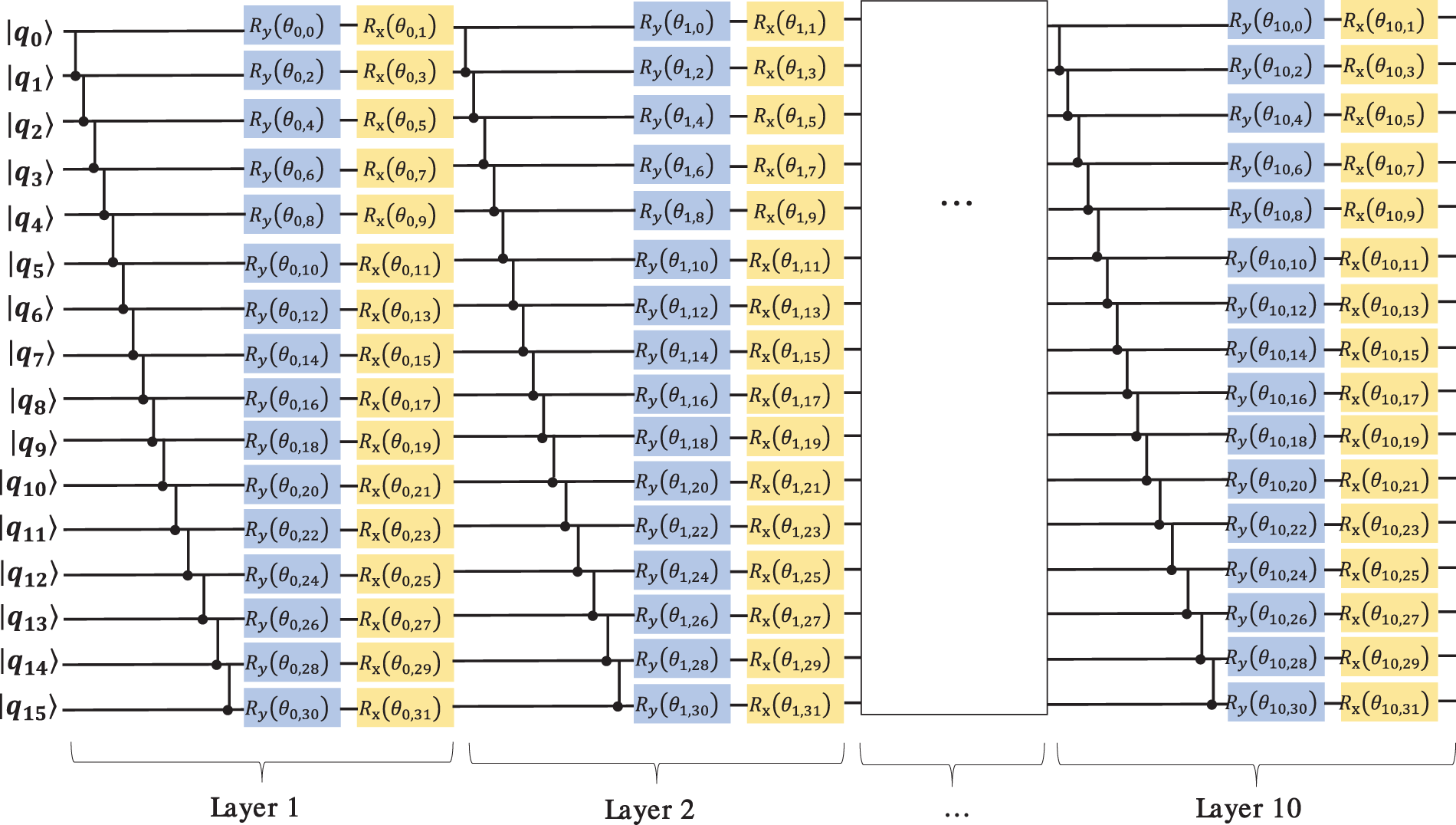
Figure 4: Parameterized quantum circuits

Similar to the generalized approximation theorem [37] for classical networks, parameterized quantum circuits can fit any objective function approximately, and thus parameterized quantum circuits are considered to be similar to the layer of connected computational units controlled by adjustable parameters in neural networks [20]. The researcher used the Fisher information matrix to measure the amount of information and used the effective dimension to evaluate the model’s ability to generalize to the data, and finally concluded that compared to classical neural networks, the Fisher information matrix features of quantum circuits are more uniformly distributed, and can consistently achieve the highest effective dimensions over a limited range of data, and thus are expected to generate models with greater capacity and stronger generalization ability [38].

Quantum Circuits Measurement Layer

The quantum circuits measurement layer extracts useful information from quantum states through quantum measurements and converts it back to classical data for further analysis and processing.

We use the TensorCircuit [39] simulator to measure the expected value of each quantum bit on the Z-axis, and these expected results are rowed into a set of measurement result vectors [E0, E1,…,En−1].

In summary, the quantum feature learning module is formulated as follows:

PQ(s, θ)=|w(θ)⟩|v(s)⟩|φini⟩(13)

where |w(θ)⟩ is a parameterized quantum circuit whose parameter θ is a matrix of [2∗L, Qbit], L is the number of cell layers, and Qbit is the number of quantum bits. |v(s)⟩ represents the quantum coding and |φini⟩ is the random initialization value.

Classical Optimization Module

The classical optimization module includes a classical fully connected layer and optimization, the vector data [E0, E1,…,En−1] obtained from the quantum circuits measurement layer is inputted to the classical optimization module, and the output of the fully connected layer is the predicted detection result, i.e., whether it is a drone or not.

We use the sigmoid function activation of the classical algorithm at the fully connected layer to normalize the output so that the prediction yields a probability between 0 and 1, which is defined as:

S(x)=11+e−x(14)

The formula for the fully connected layer is:

PC(x, θ′)=w(θ′)x+b(15)

where x is the feature vector [E0, E1,…,En−1], obtained by the quantum feature learning module.

The entire optimization process of the hybrid quantum neural networks is a back-propagation process, where the gradient of the classical fully connected layer is computed first, and then, from back to front, the gradient of the parameterized quantum line layer is computed. We use TensorFlow’s auto-differential method here to implement the solution of the parametric gradient, using the binary cross-entropy function to calculate the loss value and Adam’s algorithm for optimization.

Many quantum machine learning algorithms outperform classical algorithms on certain problems [18], bringing quantum acceleration [40]. The hybrid quantum-classical optimization algorithm is one of the most promising recent algorithms in the quantum field [41]. Parameterized quantum circuits are the counterpart of classical feed-forward neural networks in the field of quantum machine learning [42], the ability of quantum neural networks to deal with correlations between data is related to the entanglement of quantum wavefunctions, and quantum entanglement in quantum mechanics is the key to quantum classifiers; moreover, quantum classification circuits do not amplify the noise of the data and labels [43]. Quantum circuits learning has the potential to represent more complex functions than classical algorithms [19]. HQNN-SFOP is a hybrid quantum-classical optimization algorithm with a parameterized quantum circuits layer that achieves entanglement between quantum bits through the CNOT gate. Due to the superposition and entanglement properties of quantum states in Hilbert space, compared to the classical two-dimensional space, HQNN-SFOP can extract the feature information of signals in Hilbert’s high dimensional space [11], and the robustness of parameterized quantum circuits to the noise of data and labels makes them have better accuracy. Experiment 4.5 verifies that HQNN-SFOP has a stronger learning capability compared to the classical algorithm.

4  Experiments and Results

We experimentally validate the proposed use of the hybrid quantum neural networks with signal feature overlay projection (HQNN-SFOP) for detecting radar return signals from drones after extracting the statistical features of the signals in the time domain, and this section describes in detail the datasets used in the experiments, the relevant baselines, the data preprocessing process, and the results of the comparative analyses of the various experiments.

4.1 Dataset

We use the MM model to generate the dataset, which is defined as follows:

{S1:ψ(t)+υ(t)S0:υ(t)(16)

S1 represents the case of the existence of a drone, S0 represents the case of no drone only noise, in the formula ψ(t) is the drone without noise, υ(t) is the noise. This is the theory of hypothesis testing in mathematical theory, according to the verdict for the existence and non-existence of the target signal, which is a binary hypothesis testing problem. We generate a sample dataset based on this definition, and the length of each sample is 0.4 s. For this dataset, the machine learning method is used to do binary classification after extracting time domain statistical features.

The number of samples for each training dataset is 900, of which 450 are sample data generated from the parameters for five types of drones and 450 are noise sample data. The number of samples for the validation dataset is 300, with half of the sample data from the parameters for five types and half of the sample data from noise. There are three test datasets so that the standard deviation of the measurement results can be generated, and the number of sample entries for each test dataset is 300, with half each of the five drones parameter sample data and the noise sample data as well. The ratio of training set, validation set, and test set is 6:2:2.

To improve the compatibility of the model, drone sample data were also generated using random parameters, with the same number and proportion of training, validation, and test sets as above, with the difference that the five drones parameter sample data were replaced with random drones sample data.

We generated sample datasets at SNRs of 0, 5, 10, 15, and 20 dB, respectively, which are convenient for subsequent experimental analysis and comparison. In the real task, a negative SNR indicates that the noise is stronger than the signal, and this extreme case generally requires noise reduction processing to strip off the noise to optimize the signal quality before analysis, which is not in our current discussion.

4.2 Configuration

We use Tensorflow to build a neural network framework and Tensorcircuit to simulate quantum circuits. Classical machine learning algorithms such as SVM, LogisticRegression, DecisionTree, GaussianNB and BernoulliNB come from Scikit-learn. All implementations are based on the Python language.

We use 16 qubits to execute the HQNN-SFOP circuits. The training batch_size is 16 and the epoch is 6. We used the binary cross-entropy function to calculate the loss value, and the Adam algorithm with a learning rate of 0.03 was used for optimization.

4.3 Baseline

We use a baseline of metrics commonly used in machine learning, including ACC and F1-score, to provide an all-encompassing assessment of classifier results.

A confusion matrix is shown in Table 6, which contains the true and predicted classifications of the sample dataset with Positive and Negative results in the true and predicted classifications, respectively.

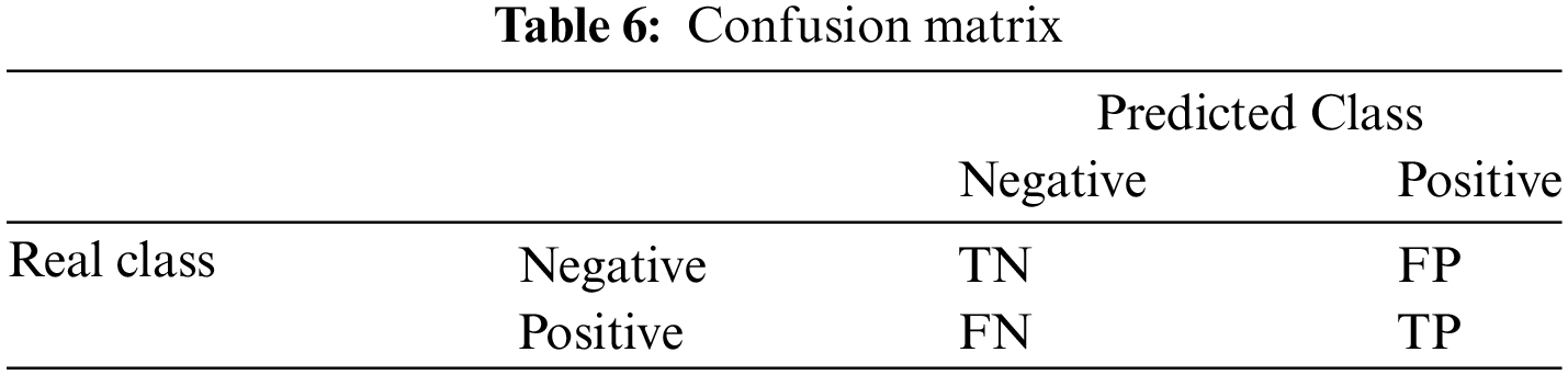
The descriptions of TP, FP, FN, and TN in the confusion matrix are as follows:

TP: represents the case where the true classification value is Positive and the predicted classification value is also Positive.

FP: represents the case where the true classification value is Negative and the predicted classification value is Positive.

FN: represents the case where the true classification value is Positive and the predicted classification value is Negative.

TN: represents the case where the true classification value is Negative and the predicted classification value is Negative.

Based on the confusion matrix above, Accuracy, Recall, Precision, and F1-score can be defined.

ACC: is the proportion of the total sample size that is correctly categorized.

ACC=TP+TNTP+FP+TN+FN(17)

In general, the larger that accuracy is, the better. In the case of unbalanced label distribution, especially in extreme cases, such as 99 out of 100 sample data are negatively labeled, then the classifier just needs to give all the predictions negative to get 99% accuracy, and this kind of classifier is not what we want, so other metrics need to be introduced.

Recall: the proportion of results actually categorized as positive samples that are predicted to be categorized as positive samples.

Recall=TPTP+FN(18)

Precision: the proportion of results predicted to be categorized as positive samples that are actually categorized as positive samples.

Precision=TPTP+FP(19)

Recall and precision represent the ability of the classifier to recognize positive and negative samples, respectively; the higher the recall, the better the ability of the classifier to recognize negative samples, and the higher the precision, the better the ability of the classifier to recognize positive samples. The use of recall or precision alone does not fully represent the performance of the classifier, precision and recall affect each other, although both are high is a desired ideal situation, however, in practice, it is often the case that the precision is high and the recall is low, or the recall is low, but the precision is high, so the F1-score is introduced to take into account the two.

F1-score: the harmonic mean of precision and recall.

F1−score=2∗Precision∗RecallPrecision+Recall(20)

4.4 Data Pre-Processing and Feature Selection

The features of the signal sample dataset after feature extraction are not uniformly distributed. To avoid the learning results being biased towards some of the features with obvious eigenvalues, it is necessary to standardize the sample dataset to make the various features of the sample dataset more comparable with each other. We use the classical algorithm of StandardScaler for the process, which standardizes the features by removing the mean and scaling by standard variance to facilitate the subsequent quantum coding.

Researchers’ experiments have shown that choosing a finite feature set that accurately indicates the characteristics of the data outperforms a large-scale feature set, because a larger feature set introduces more noise and may also make the model overly focused on the training data [10]. Therefore, the feature set needs to be selected.

We use the Pearson correlation coefficient method [44] to analyze the strength of linear correlation between time-domain features extracted from the drones dataset and the labels in order to filter the feature set. The Pearson correlation coefficient method is defined as follows:

r=∑(x−x¯)(y−y¯)∑(x−x¯)2∑(y−y¯)2(21)

where x is the time domain feature, y is the label, and r is the correlation coefficient between x and y. r > 0 is a positive correlation, r < 0 is a negative correlation, and r = 0 means there is no correlation between the two. Features positively correlated with labels are shown in Fig. 5.

Figure 5: Correlation coefficients for each feature

Analyzing the correlation coefficients of these time-domain features in Fig. 5, the correlation coefficients of two features, Margin-real and Pulse-real, are greater than 60%, and the correlation coefficients of four features, Max-real, Minimum-real, Peak, and Peak-to-peak-real, are greater than 40%. We choose time domain features with correlation coefficients greater than 5%. In addition, there are some features such as Max, Margin, and Pulse, whose correlation coefficients are more than 5% for their real values and less than 5% for their imaginary values, and some features such as Median and Mean, whose correlation coefficients are more than 5% for their imaginary values and less than 5% for their real values. To ensure the completeness of the signals, both the real and the imaginary parts of these features are retained, resulting in a 16-dimensional feature.

Finally, the 16-dimensional time-domain features are used for the feature extraction of radar return signals from drones, and the sample dataset generated from them was fed into the hybrid quantum neural networks for computation.

4.5 Advantages over Classical Machine Learning Algorithms

We use the classical machine learning algorithms SVM [45], LogisticRegression [46], DecisionTree [47], GaussianNB [48], BernoulliNB [49], NN [50], and the hybrid quantum machine learning algorithm HQNN-SFOP to perform experiments on the 16-dimensional signal time-domain statistical features extracted from the radar return signal dataset with an SNR of 10 dB. Both the training and test sets are radar return signal datasets generated from five drones parameters. The difference between NN and HQNN-SFOP is that the quantum feature learning module of HQNN-SFOP is replaced with the fully connected layer of the classical neural networks, while the other parts such as the classical optimization module and the training parameters are kept the same.

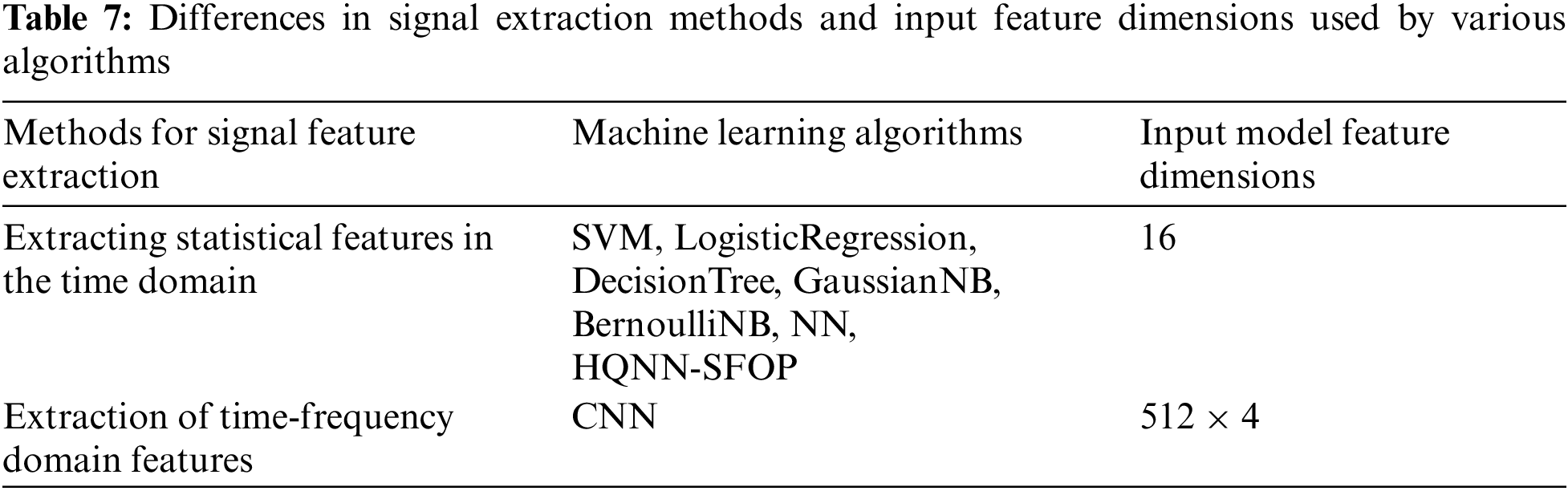
In addition, we introduce the results of the CNN method mentioned in the paper [24] for comparison, which also uses the same radar return signal dataset, extracts time-frequency domain features on the signals to generate spectrograms, and achieves the target detection by image recognition of the spectrograms with the dimension of 512 × 4 by CNN. The differences in signal extraction methods and input feature dimensions used by the various algorithms are shown in Table 7, and the experimental results are shown in Table 8.

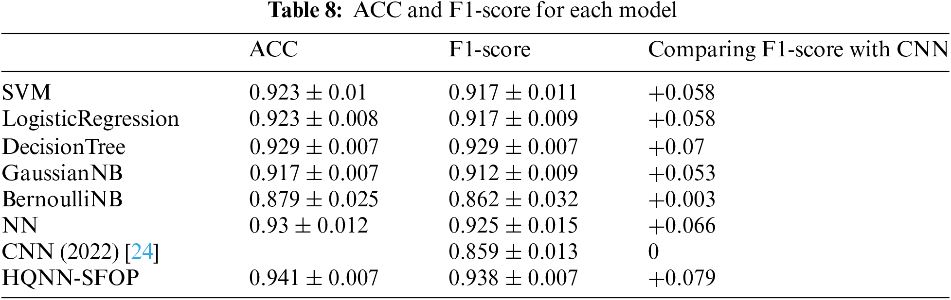
Analyzing the experimental results, it can be seen that the F1-scores of SVM, LogisticRegression, DecisionTree, GaussianNB, BernoulliNB, NN, and HQNN-SFOP for time-domain statistical features are better than the F1-score of the CNN method for spectrogram identification, which is 0.859 ± 0.013, and it indicates the effectiveness of our extracted time-domain statistical features for drone detection using radar return signals. This effectiveness proves that the extracted time-domain features are sufficient to express the signal characteristics, while the precise selection of the features avoids the noise interference that may result from too many features.

On the other hand, compared to other classical methods, HQNN-SFOP has the highest ACC value and F1-score of 0.941 ± 0.007 and 0.938 ± 0.007, respectively, which are also higher than those of 0.93 ± 0.012 and 0.925 ± 0.015 for NN, which are improved by 0.011 and 0.013, respectively. This validates that the introduction of quantum circuits in the HQNN-SFOP method improves the neural network’s ability to acquire feature inline relations and improves the accuracy of drone detection using radar return signals.

We use 5-fold cross-validation to calculate the ACC value and F1-score of each model. The SNR of the sample data set is 10 dB, the extracted signal time-domain statistical features are 16-dimensional, and the number of samples is 1200. 5-fold cross-validation randomly divides the sample data set into five parts, each time randomly selects four parts as the training set and one part as the test set. The ratio of the training set and test set is 4:1, and the ACC value and F1-score of the model are calculated using this training set and test set. This operation is repeated five times, and the average of the five test results is calculated, which is used to evaluate the accuracy of the model. The experimental results are shown in Table 9.

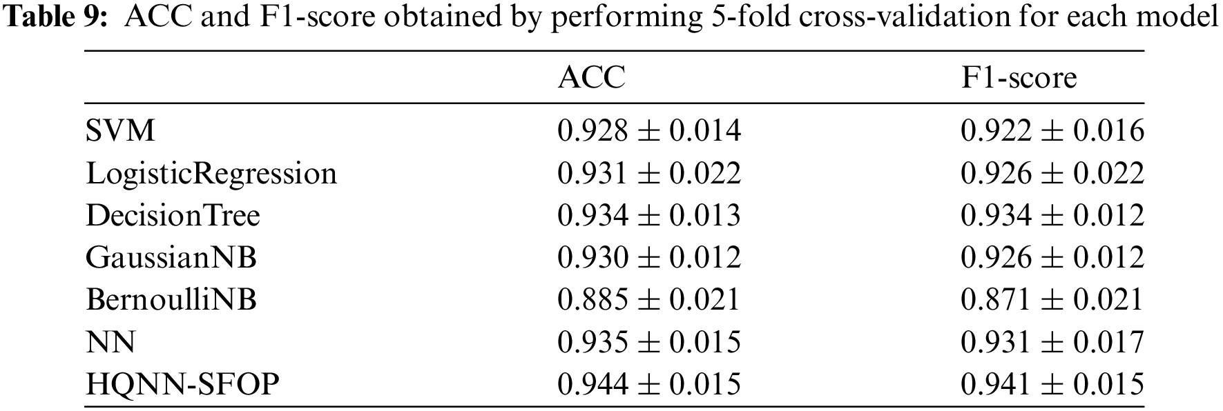
By analyzing the experimental results of the 5-fold cross-validation, it can be found that compared with other methods, HQNN-SFOP has the highest ACC value and F1-score, which are 0.944 ± 0.015 and 0.941 ± 0.015, respectively, thus verifying the performance advantage of HQNN-SFOP from a statistical point of view.

This set of experiments illustrates that the HQNN-SFOP method has significant advantages on the radar return signal dataset, both in terms of statistical feature extraction in the time domain and terms of signal detection capability, realizing the extraction of a smaller set of features yet obtaining the highest drone detection accuracy.

4.6 Migration Generalization Ability at Different SNRs

We trained and tested the five types of drones datasets and the random drones datasets with SNRs of 0, 5, 10, 15, and 20 dB, respectively, and conducted cross-testing experiments between these datasets, that is, the model generated by the training of the five types of drones dataset was tested not only with the five types of drones dataset, but also tested with the random drones dataset, and the model trained by the random drones dataset training was also the same, so as to verify its migration generalization ability, and the results are shown in Fig. 6. where 5Dro is the dataset generated from the five types of drones parameters, and RDro is the dataset generated from the random drones parameters.

Figure 6: F1-score of HQNN-SFOP for five drones datasets and random drones datasets at different SNRs

Analyzing Fig. 6, both HQNN-SFOPs perform well and undergo a linearly increasing change with increasing SNR. The F1-score for both self-validation and cross-validation exceeds 0.85 for SNR greater than or equal to 5 dB. The F1-score for both self-validation and cross-validation exceeds 0.90 for SNR greater than or equal to 10 dB. And the F1-score for both self-validation and cross-validation exceeds 0.94 for SNR greater than or equal to 15 dB. Even though the SNR is 0 dB, the F1-score for both self-validation and cross-validation of HQNN-SFOP exceeds 0.80. In contrast, compared to the classical image detection CNN algorithm [24], the F1-score for both self-validation and cross-validation for an SNR of 0 dB is only as high as 0.5. The F1-score for both self-validation and cross-validation for an SNR equal to 5 dB is around 0.60. When SNR is equal to 10 dB, its F1-score for self-validation and cross-validation is around 0.85. When SNR is equal to 15 dB, only one set of its F1-score for self-validation and cross-validation reaches 0.9 and the rest of them are below 0.9.

The F1-score of HQNN-SFOP outperforms the results of CNN at SNRs of 0, 5, 10, 15, and 20 dB, respectively, and the F1-scores generalized to other data type datasets at the same SNR are all stable. The experiments show that HQNN-SFOP has a strong migration generalization ability, and compared with CNN, HQNN-SFOP has a stronger feature expression ability and migration generalization ability.

4.7 Ablation Experiment

4.7.1 Advantages of HQNN-SFOP Compared with NN

In this section of experiments, we test HQNN-SFOP and NN on the drone datasets to discuss the advantages of hybrid quantum neural networks over classical neural networks. In this case, NN replaces the quantum feature learning module of HQNN-SFOP with the fully connected layer of the classical neural networks, while other configurations such as the classical optimization module and the training parameters are the same for NN and HQNN-SFOP.

Both HQNN-SFOP and NN are trained on five drones datasets and tested on five drones datasets and random drones datasets with SNRs of 0, 5, 10, 15, and 20 dB, respectively. The F1-score results of their tests are summarized in Fig. 7.

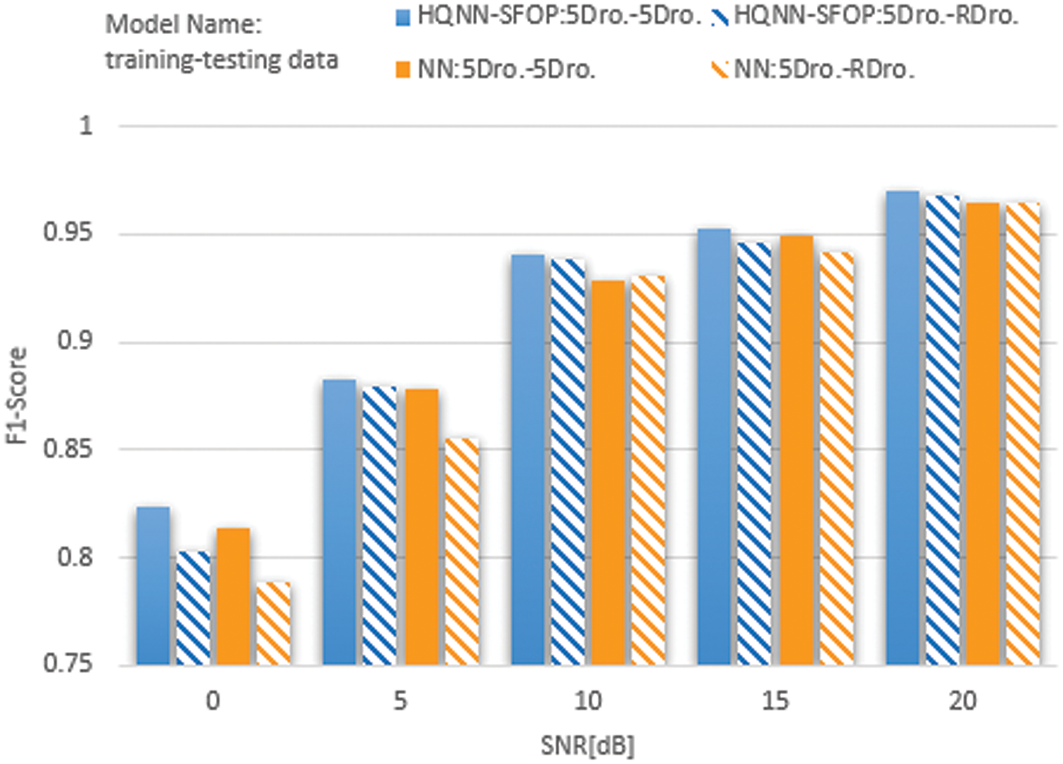
Figure 7: F1-score of HQNN-SFOP, NN for five drones datasets and random drones datasets at different SNRs

In Fig. 7, HQNN-SFOP is the F1-score result of our hybrid quantum neural networks with signal feature overlay projection, and NN is the F1-score result of the classical neural networks. The results of HQNN-SFOP are higher than those of NN on both the tests on the five drones datasets and the random drones datasets. As the signal noise increases, this advantage becomes more pronounced at SNRs less than 10, especially in the results for the test set of random drones datasets. This shows that the hybrid quantum neural network with signal feature overlay projection can improve the ability of the neural network to acquire feature inline relations, and its stability and mobility are stronger in a high-noise environment.

Through the experiments in this subsection, we deeply demonstrate the advantages of the hybrid quantum neural networks with signal feature overlay projection over the classical neural networks for radar return signals from drones and prove that HQNN-SFOP has stronger feature inline relationship acquisition and migration generalization ability, which is more obvious in high-noise environments.

4.7.2 Advantages Offered by Signal Feature Overlay Projection

In this section of experiments, we investigate the effect of signal feature overlay projection on the training results. We remove the signal feature overlay projection to test the sample dataset for inspection and testing and compare the test results with and without signal feature overlay projection, respectively, and both use five drones datasets for training, five drones datasets and random drones datasets for testing, and the results are shown in Fig. 8.

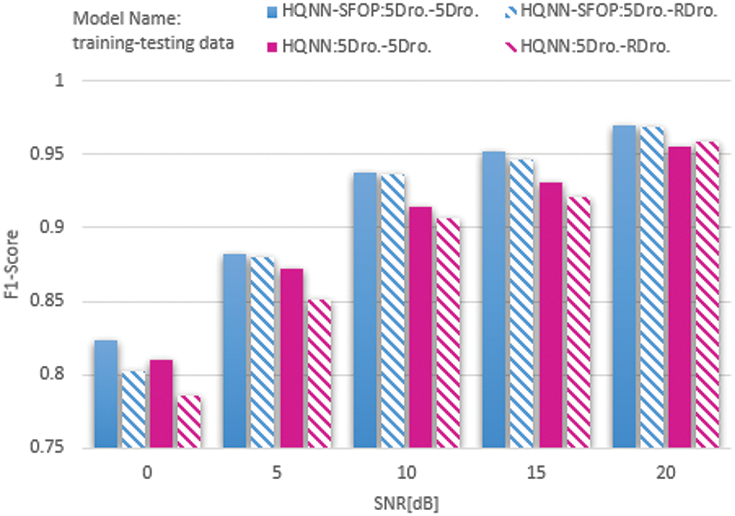
Figure 8: F1-score of HQNN-SFOP, HQNN for five drones datasets and random drones datasets at different SNRs

In Fig. 8, HQNN-SFOP is the test result using signal feature overlay projection, and HQNN is the result without signal feature overlay projection. Analyzing the comparison results, the results of HQNN-SFOP are better than those of HQNN for the same training set and test set with SNR of 0, 5, 10, 15, and 20 dB, respectively, regardless of whether the test set is the five drones dataset or the random drones dataset. This indicates that the use of signal feature overlay projection does play a role in improving feature representation. This enhancement comes from the Bloch sphere layer expansion brought about by the rotation of quantum bits.

4.7.3 Compare Different Quantum Circuits

In this experiment, we study the performance differences between quantum circuits composed of different cell layer topologies and different stacking times (i.e., cell layer numbers). Both ablation experiments were trained using five drones datasets and tested using five drones datasets and random drones datasets.

The first is the experiment with different cell layer topologies. We replace the Ry(θ), Rx(θ) topology in the quantum circuits of HQNN-SFOP with the Rx(θ), Ry(θ) topology, the Ry(θ), Ry(θ) topology, and the Rx(θ), Rx(θ) topology (Fig. 9), and train and test the sample data set, respectively. The test results of different cell layer topologies are compared with the F1-score of HQNN-SFOP, and the results are shown in Fig. 10.

Figure 9: Different cell layer topologies. (a) Ry(θ), Rx(θ) topology used by HQNN-SFOP. (b) Rx(θ), Ry(θ) topology. (c) Ry(θ), Ry(θ) topology. (d) Rx(θ), Rx(θ) topology

Figure 10: F1-score of hybrid quantum neural networks with different cell layer topologies and HQNN-SFOP for five drones datasets and random drones datasets at different SNRs

The second is the experiment of different cell layers. We replace the number of cell layers in the quantum circuits of HQNN-SFOP from 10 layers to 4 layers, 6 layers and 8 layers, and carry out training and testing on different cell layers respectively. The comparison between the test results of different numbers of cell layers and HQNN-SFOP is shown in Fig. 11.

Figure 11: F1-score of hybrid quantum neural networks with different numbers of cell layers and HQNN-SFOP for five drones datasets and random drones datasets at different SNRs

We analyze the results of two experiments. In Fig. 10, Ry(θ), Rx(θ) are the cell layer topology of HQNN-SFOP. At different SNRs, using the same training set and test set, the F1-score of HQNN-SFOP is superior to the hybrid quantum neural networks composed of other cell layer topologies, regardless of whether the test set is five drones dataset or random drones dataset. In Fig. 11, 10 is the number of cell layers of HQNN-SFOP, and its F1-score is also better than that of the mixed quantum neural networks with 4, 6 and 8 layers. These two experimental results verify that the cell layer topology and cell layer number used by HQNN-SFOP can better learn the correlation between the data features of the sample dataset.

Through the experiments in this subsection, we provide an in-depth demonstration of the advantages of the signal feature superposition over the projected feature expressivity and clearly show the contribution of the method in the overall performance, proving that the advantages of quantum superposition over information are still valid in the field of signal analysis.

5  Conclusion

For the problem that the existing drone detection relies on the time-frequency domain feature spectrogram identification to bring about the feature dimension is large, and the introduction of time-domain statistical features to reduce the dimensionality but the detection accuracy is not high, this paper innovatively proposes a signal detection method based on a new hybrid quantum neural network with signal feature overlay projected HQNN-SFOP, which unfolds the feasibility of drone detection using radar return signals to validate and analyze. Through comparison experiments with multiple classical machine learning methods and CNNs oriented to spectrogram recognition on the simulated datasets, it is proved that HQNN-SFOP achieves the highest detection accuracy and F1-score with the extraction of smaller-sized features. On the one hand, it reflects the advantage of quantum computing technology over traditional computing in terms of feature inline relationship capability acquisition, and on the other hand, it also verifies that accurately extracted high-correlation time-domain features can effectively improve the accuracy of drone detection, which is because when extracted time-domain features are sufficient to characterize the radar return signals from drones, the larger-scale spectrogram features will bring more noise, and may also make the model overly concerned with the training data, instead affecting the learning ability of the machine learning algorithm. However, there are some limitations of this time-domain feature extraction method. Firstly, although the time domain features can reflect the transformation of the signal over time, it is difficult to analyze the change of frequency and phase of the signal in the frequency domain. For some signals whose time-domain features are not obvious or whose time-domain features are not enough to express their characteristics, such as signals with complex waveform patterns or non-periodic signals, it becomes difficult to detect them only by relying on the time-domain features, and it is necessary to introduce the frequency-domain features to assist in the analysis. Secondly, when extracting some time-domain features, the whole signal needs to be traversed and calculated, which may affect the detection timeliness of some long signals. Therefore, it is necessary to reasonably screen effective features for signal detection in conjunction with the actual situation of the task.

The migration generalization ability of HQNN-SFOP is verified by cross-test experiments on five drones datasets and random drones datasets with different SNRs. It is demonstrated through ablation study that HQNN-SFOP in Hilbert space has stronger feature inline relation acquisition and migration generalization ability than NN. The enhancement of feature expression ability by signal feature overlay projection in quantum space is deeply demonstrated by the ablation study, which proves that the advantage of quantum superposition of information is still effective in the field of signal analysis, and provides a reference for the subsequent related research.

Although this paper only detects and verifies the data of radar return signals from drones, it still reflects the great potential of quantum computing technology in signal intelligent analysis, which also provides a feasible technical path for the subsequent cross-fertilization of quantum computing technology and signal analysis.

At present, HQNN-SFOP only analyzes hypothetical environments on simulated datasets, which is mainly due to the difficulty of obtaining large amounts of real drone data for training. The present work is only a preliminary exploration of drone detection using our method. Next, we need to collect real data to verify the detection capability of HQNN-SFOP on various drones in real environments, and further explore the robustness of HQNN-SFOP in detecting radar return signals from drones in various uncontrollable scenarios that may be brought about by noise, weather conditions, terrain differences, and radar equipment status in real environments. Although we enrich the sample data with random drones parameters and simulated noise, we will also face challenges brought by new data and interference in actual deployment, and we need to transfer learning or optimize the model according to the actual situation. In addition, we will further expand the research on signal detection at low SNR, signal classification, etc., to provide new methods for traditional signal analysis.

Acknowledgement: The authors would like to express their gratitude for the valuable feedback and suggestions provided by all the anonymous reviewers and the editorial team.

Funding Statement: This work is supported by Major Science and Technology Projects in Henan Province, China, Grant No. 221100210600.

Author Contributions: Study conception and design: Wenxia Wang, Xiaodong Ding; data collection: Jinchen Xu; analysis and interpretation of results: Wenxia Wang, Zhihui Song, Yizhen Huang; draft manuscript preparation: Wenxia Wang, Jinchen Xu, Xin Zhou, Zheng Shan. All authors reviewed the results and approved the final version of the manuscript.

Availability of Data and Materials: The authors confirm that the data supporting the findings of this study are available in “Detecting drones with radars and convolutional networks based on micro-Doppler signatures” [24] and its supplementary materials. Additional materials supporting the findings of this study are available from the corresponding author, Zheng Shan, upon reasonable request.

Ethics Approval: Not applicable.

Conflicts of Interest: The authors declare that they have no conflicts of interest to report regarding the present study.

References

1. Y. Wu, S. Wu, and X. Hu, “Cooperative path planning of UAVs & UGVs for a persistent surveillance task in urban environments,” IEEE Internet Things J., vol. 8, no. 6, pp. 4906–4919, Mar. 2021. doi: 10.1109/JIOT.2020.3030240. [Google Scholar] [CrossRef]

2. K. Dorling, J. Heinrichs, G. G. Messier, and S. Magierowski, “Vehicle routing problems for drone delivery,” IEEE Trans. Syst., Man, Cybern.: Syst., vol. 47, no. 1, pp. 70–85, Jan. 2017. doi: 10.1109/TSMC.2016.2582745. [Google Scholar] [CrossRef]

3. A. M. Johnson, C. J. Cunningham, E. Arnold, W. D. Rosamond, and J. K. Zègre-Hemsey, “Impact of using drones in emergency medicine: What does the future hold?,” Open Access Emerg. Med., vol. 13, pp. 487–498, Nov. 2021. doi: 10.2147/OAEM.S247020. [Google Scholar] [PubMed] [CrossRef]

4. J. Scott and C. C. Scott, “Drone delivery models for healthcare,” presented at the 50th Hawaii Int. Conf. Syst. Sci., Waikoloa, HI, USA, Jan. 4–7, 2017. [Google Scholar]

5. X. Xu et al., “An automatic wheat ear counting model based on the minimum area intersection ratio algorithm and transfer learning,” Measurement, vol. 216, Jul. 2023, Art. no. 112849. [Google Scholar]

6. L. Tang and G. Shao, “Drone remote sensing for forestry research and practices,” J. For. Res., vol. 26, pp. 791–797, Jun. 2015. doi: 10.1007/s11676-015-0088-y. [Google Scholar] [CrossRef]

7. A. Coluccia, G. Parisi, and A. Fascista, “Detection and classification of multirotor drones in radar sensor networks: A review,” Sensors, vol. 20, no. 15, Jul. 2020, Art. no. 4172. [Google Scholar]

8. S. Rahman and D. A. Robertson, “Radar micro-Doppler signatures of drones and birds at K-band and W-band,” Sci. Rep., vol. 8, p. 2, Nov. 2018. doi: 10.1038/s41598-018-35880-9. [Google Scholar] [PubMed] [CrossRef]

9. D. Raval, E. Hunter, S. Hudson, A. Damini, and B. Balaji, “Convolutional neural networks for classification of drones using radars,” Drones, vol. 5, no. 4, Dec. 2021. doi: 10.3390/drones5040149. [Google Scholar] [CrossRef]

10. S. Bolton, R. Dill, M. R. Grimaila, and D. Hodson, “ADS-B classification using multivariate long short-term memory-fully convolutional networks and data reduction techniques,” J. Supercomput., vol. 79, pp. 2281–2307, Feb. 2023. doi: 10.1007/s11227-022-04737-4. [Google Scholar] [CrossRef]

11. C. Bennett and D. DiVincenzo, “Quantum information and computation,” Nature, vol. 404, pp. 247–255, Mar. 2000. doi: 10.1038/35005001. [Google Scholar] [PubMed] [CrossRef]

12. M. Cerezo et al., “Variational quantum algorithms,” Nat. Rev. Phys., vol. 3, no. 9, pp. 625–644, Aug. 2021. doi: 10.1038/s42254-021-00348-9. [Google Scholar] [CrossRef]

13. S. Lee et al., “Evaluating the evidence for exponential quantum advantage in ground-state quantum chemistry,” Nat. Commun., vol. 14, Apr. 2023, Art. no. 1952. doi: 10.1038/s41467-023-37587-6. [Google Scholar] [PubMed] [CrossRef]

14. H. Y. Huang et al., “Quantum advantage in learning from experiments,” Science, vol. 376, pp. 1182–1186, Jun. 2022. doi: 10.1126/science.abn7293. [Google Scholar] [PubMed] [CrossRef]

15. J. Preskill, “Quantum computing in the NISQ era and beyond,” Quantum, vol. 2, Aug. 2018, Art. no. 79. doi: 10.22331/q-2018-08-06-79. [Google Scholar] [CrossRef]

16. D. Ristè et al., “Demonstration of quantum advantage in machine learning,” npj Quantum Inf., vol. 3, no. 1, Apr. 2017, Art. no. 16. doi: 10.1038/s41534-017-0017-3. [Google Scholar] [CrossRef]

17. H. Y. Huang, R. Kueng, and J. Preskill, “Information-theoretic bounds on quantum advantage in machine learning,” Phys. Rev. Lett., vol. 126, no. 19, May 2021, Art. no. 190505. doi: 10.1103/PhysRevLett.126.190505. [Google Scholar] [PubMed] [CrossRef]

18. J. Biamonte et al., “Quantum machine learning,” Nature, vol. 549, pp. 195–202, Jul. 2017. doi: 10.1038/nature23474. [Google Scholar] [PubMed] [CrossRef]

19. K. Mitarai, M. Negoro, M. Kitagawa, and K. Fujii, “Quantum circuit learning,” Phys. Rev. A, vol. 98, no. 3, Sep. 2018, Art. no. 032309. doi: 10.1103/PhysRevA.98.032309. [Google Scholar] [CrossRef]

20. M. Benedetti, E. Lloyd, S. Sack, and M. Fiorentini, “Parameterized quantum circuits as machine learning models,” Quant. Sci. Technol., vol. 4, no. 4, Nov. 2019. doi: 10.1088/2058-9565/ab4eb5. [Google Scholar] [CrossRef]

21. J. Martin and B. Mulgrew, “Analysis of the effects of blade pitch on the radar return signal from rotating aircraft blades,” in 92 Int. Conf. Radar, Brighton, UK, 1992, pp. 446–449. [Google Scholar]

22. A. French, Target Recognition Techniques for Multifunction Phased Array Radar. London, UK: University College London, 2010. [Google Scholar]

23. S. Hudson and B. Balaji, “Application of machine learning for drone classification using radars,” in Signal Process., Sens./Inform. Fusion, Target Recognit. XXX, Apr. 2021, vol. 11756, pp. 72–84. doi: 10.1117/12.2588694. [Google Scholar] [CrossRef]

24. D. Raval, E. Hunter, I. Lam, S. Rajan, A. Damini and B. Balaji, “Detecting drones with radars and convolutional networks based on micro-Doppler signatures,” in RadarConf22, New York City, NY, USA, 2022, pp. 1–6. [Google Scholar]

25. Z. Shi, X. Chang, C. Yang, Z. Wu, and J. Wu, “An acoustic-based surveillance system for amateur drones detection and localization,” IEEE Trans. Veh. Technol., vol. 69, no. 3, pp. 2731–2739, Mar. 2020. doi: 10.1109/TVT.2020.2964110. [Google Scholar] [CrossRef]

26. M. Z. Anwar, Z. Kaleem, and A. Jamalipour, “Machine learning inspired sound-based amateur drone detection for public safety applications,” IEEE Trans. Veh. Technol., vol. 68, no. 3, pp. 2526–2534, Mar. 2019. doi: 10.1109/TVT.2019.2893615. [Google Scholar] [CrossRef]

27. B. Taha and A. Shoufan, “Machine learning-based drone detection and classification: State-of-the-art in research,” IEEE Access, vol. 7, pp. 138669–138682, Sep. 2019. [Google Scholar]

28. C. Aker and S. Kalkan, “Using deep networks for drone detection,” in 2017 14th IEEE Int. Conf. Adv. Video Signal Based Surveill. (AVSS), Lecce, Italy, 2017, pp. 1–6. [Google Scholar]

29. M. Jahangir and C. Baker, “Robust detection of micro-UAS drones with L-band 3-D holographic radar,” in SSPD, Edinburgh, UK, 2016, pp. 1–5. [Google Scholar]

30. C. Wang, J. Tian, J. Cao, and X. Wang, “Deep learning-based UAV detection in pulse-Doppler radar,” IEEE Trans. Geosci. Remote Sens., vol. 60, pp. 1–12, Aug. 2022. doi: 10.1109/TGRS.2021.3104907. [Google Scholar] [CrossRef]

31. J. Gérard, J. Tomasik, C. Morisseau, A. Rimmel, and G. Vieillard, “Micro-Doppler signal representation for drone classification by deep learning,” in 2020 28th Eur. Signal Process. Conf. (EUSIPCO), Amsterdam, Netherlands, 2021, pp. 1561–1565. [Google Scholar]

32. Y. Lecun, L. Bottou, Y. Bengio, and P. Haffner, “Gradient-based learning applied to document recognition,” Proc. IEEE, vol. 86, no. 11, pp. 2278–2324, Nov. 1998. [Google Scholar]

33. H. Xiao, K. Rasul, and R. Vollgraf, “Fashion-MNIST: A novel image dataset for benchmarking machine learning algorithms,” Sep. 2017. doi: 10.48550/arXiv.1708.07747. [Google Scholar] [CrossRef]

34. B. Boashash, Time-Frequency Signal Analysis and Processing: A Comprehensive Reference. New York, NY, USA: Academic Press, 2015. [Google Scholar]

35. A. Pérez-Salinas, A. Cervera-Lierta, E. Gil-Fuster, and J. I. Latorre, “Data re-uploading for a universal quantum classifier,” Quantum, vol. 4, Feb. 2020, Art. no. 226. doi: 10.22331/q-2020-02-06-226. [Google Scholar] [CrossRef]

36. M. Schuld, R. Sweke, and J. J. Meyer, “Effect of data encoding on the expressive power of variational quantum-machine-learning models,” Phys. Rev. A, vol. 103, Mar. 2021, Art. no. 032430. doi: 10.1103/PhysRevA.103.032430. [Google Scholar] [CrossRef]

37. K. Hornik, M. Stinchcombe, and H. White, “Multilayer feedforward networks are universal approximators,” Neural Netw., vol. 2, no. 5, pp. 359–366, Jan. 1989. doi: 10.1016/0893-6080(89)90020-8. [Google Scholar] [CrossRef]

38. A. Abbas, D. Sutter, C. Zoufal, A. Lucchi, A. Figalli and S. Woerner, “The power of quantum neural networks,” Nat. Comput. Sci., vol. 1, pp. 403–409, Jun. 2021. doi: 10.1038/s43588-021-00084-1. [Google Scholar] [PubMed] [CrossRef]

39. S. X. Zhang et al., “TensorCircuit: A quantum software framework for the NISQ era,” Quantum, vol. 7, Feb. 2023, Art. no. 912. doi: 10.22331/q-2023-02-02-912. [Google Scholar] [CrossRef]

40. M. Schuld, I. Sinayskiy, and F. Petruccione, “An introduction to quantum machine learning,” Contemp. Phys., vol. 56, pp. 172–185, Oct. 2014. doi: 10.1080/00107514.2014.964942. [Google Scholar] [CrossRef]

41. L. Banchi and G. E. Crooks, “Measuring analytic gradients of general quantum evolution with the stochastic parameter shift rule,” Quantum, vol. 5, Jan. 2021, Art. no. 386. doi: 10.22331/q-2021-01-25-386. [Google Scholar] [CrossRef]

42. W. Vinci and A. Shabani, “Optimally stopped variational quantum algorithms,” Phys. Rev. A, vol. 97, no. 4, Apr. 2018, Art. no. 042346. doi: 10.1103/PhysRevA.97.042346. [Google Scholar] [CrossRef]

43. M. Schuld, A. Bocharov, K. M. Svore, and N. Wiebe, “Circuit-centric quantum classifiers,” Phys. Rev. A, vol. 101, no. 3, Mar. 2020, Art. no. 032308. doi: 10.1103/PhysRevA.101.032308. [Google Scholar] [CrossRef]

44. J. Benesty, J. Chen, Y. Huang, and I. Cohen, “Pearson correlation coefficient,” Noise Reduct. Speech Process., vol. 2, pp. 1–4, Mar. 2009. doi: 10.1007/978-3-642-00296-0_5. [Google Scholar] [CrossRef]

45. M. Mohammadi et al., “A comprehensive survey and taxonomy of the SVM-based intrusion detection systems,” J. Netw. Comput. Appl., vol. 178, 2021, Art. no. 102983. doi: 10.1016/j.jnca.2021.102983. [Google Scholar] [CrossRef]

46. A. Bailly et al., “Effects of dataset size and interactions on the prediction performance of logistic regression and deep learning models,” Comput. Methods Programs Biomed., vol. 213, Jan. 2022, Art. no. 106504. doi: 10.1016/j.cmpb.2021.106504. [Google Scholar] [PubMed] [CrossRef]

47. B. Charbuty and A. Abdulazeez, “Classification based on decision tree algorithm for machine learning,” JASTT, vol. 2, no. 1, pp. 20–28, Mar. 2021. doi: 10.38094/jastt20165. [Google Scholar] [CrossRef]

48. Z. Ding, J. Guo, Z. Shao, and H. Zhu, “A Radar classification system based on Gaussian NB,” in 2022 Int. Conf. Intell. Transp., Big Data Smart City (ICITBS), Hengyang, China, 2022, pp. 12–15. [Google Scholar]

49. W. Yu and Y. Huang, “Research on classification algorithm for Blackberry Lily data,” J. Phys.: Conf. Series, vol. 1607, no. 1, 2020, Art. no. 012099. doi: 10.1088/1742-6596/1607/1/012099. [Google Scholar] [CrossRef]

50. J. T. Hancock and T. M. Khoshgoftaar, “Survey on categorical data for neural networks,” J. Big Data, vol. 7, Mar. 2020, Art. no. 28. doi: 10.1186/s40537-020-00305-w. [Google Scholar] [CrossRef]