Unknown Environment Measurement Mapping by Unmanned Aerial Vehicle Using Kalman Filter-Based Low-Cost Estimated Parallel 8-Beam LIDAR

1  Introduction

An unmanned aerial vehicle (UAV) is mostly utilized in military, commercial, civil, and agricultural applications owing to its inherent advantages compared to aerial vehicles with pilots. The mapping and detection of targets are critical for many applications of UAVs such as search and rescue, object transportation, object detection, inspection, and mapping [1]. The signal information from sensors can help lock the target in an efficient way [2]. It attempted to perform mapping of the riverine landscape using UAV technology encompassing all the aspects of flight mission logistics, data acquisition, and processing. The proposed approach can minimize geometric errors and enhance accuracy [3]. An approach was proposed to create an information map that consists of uncertain aimed locations and develop the optimal paths using combined global coordinates with local images gathered from UAV [4]. Further, UAVs are often used for target detection using a camera with the help of the YOLO algorithm as discussed in [5]. An investigation was made with automatic fixed-wing UAV carrier landing using model predictive control under the consideration of carrier deck motions. The automatic carrier landing was performed sequentially by two types of control systems to enhance the performance of Shipboard Landing [6]. The application of filtering algorithms on high-resolution point cloud data collection from UAV could help to attain 93% of the accuracy of the real-time data [7]. It was found that the addition of Ground Control Points (GCPs) would further increase the precision of low-cost UAVs. This can reduce the uncertainty of the ground mapping [8]. An automatic OBIA algorithm was developed by deriving photogrammetric point clouds using UAV in almond orchards. The maps for almond tree volume and volume growth were successfully created [9]. Due to the wide availability of UAVs and their ease of use, the number of operators with limited surveying and photogrammetric knowledge is being constantly increased. It has been found that the fixed wing could be faster and cover large areas while the copter could give better-resolution images at lower heights [10]. UAV LiDAR point clouds vary in response to key UAV flight parameters but are robust and predictable at the site level and target levels. A novel approach has been presented in UAVs using LiDAR data processing to remove extraneous points [11]. The MIMO Radar with UAV can be used to predict the early trajectory accurately with the help of an algorithm spatial-temporal integrated framework [12]. The potential use of UAVs for air quality research has been established with sensors. The challenges such as the type of sensor, sensor sensitivity, and payload of UAV are addressed. These challenges are not simply technological, in fact, policies and regulations, which differ from one country to another [13]. The tracking and locking of the target object are very much important for the three-dimensional object scene reconstruction. It is possible with the integration of the different sensors to meet the objectives. The integration of sensor information can enhance the measurement process in an efficient way [14]. It has been observed that a lot of works have to be carried out to optimize the vertical accuracy [15].

When compared to conventional platforms like satellite and manned aircraft, UAV-based platforms can minimize operating time. The LiDAR can efficiently scan better surface topography using UAV [16]. Civil structures can be efficiently reconstructed using LiDAR-assisted UAVs [17]. A greedy algorithm is helpful to generate and create waypoints with optimized coverage for scanning purposes [18]. The building information models have been efficient with the optimal planning of UAV paths [19]. It has been evident that it is necessary to make a detailed study of the locations of GCPs in order to maximize the accuracy obtained in photogrammetric projects [20]. The evaluation of UAV mapping should be performed to check the accuracy of scanning using LiDAR [21]. The effect of the UAV’s altitude can be an influential factor in determining civil environments [22]. The UAV could able to scan and map the agricultural field surveying and river landscape with higher accuracy of mapping [23]. The various types of geohazards could be easily monitored and mapped using LiDAR-assisted UAVs [24]. The extended Kalman filter could be utilized to predict and track the position of the vehicle with the help of the reliability function [25]. The tightly-coupled iterated Kalman filter can predict the Kalman gain to predict indoor and outdoor environments [26]. The Kalman filter could perform enhanced mapping and present a cost-effective substitute to traject the wake movement [27]. It was observed that Kalman filter-based UAV movement can reconstruct any environment under higher mapping accuracy [28]. The possibility of the mapping using LiDAR has been explained in the work [29] and the mapping is successfully generated using LiDAR. In all studies, the usage of LiDAR with a single beam with a complex algorithm has been studied. With a single beam, a UAV covers the intended measurement site with a larger number of cycles. Moreover, the measured mappings are subjected to noise vulnerability and jerks as LiDAR fitted in the UAV.

From the literature, it was observed that only very few studies were conducted on the mapping of unknown environments using the reconstruction principle with the help of UAVs using 8-beam LiDAR. Hence the present investigation was proposed. In the present study, an attempt has been made to design 8 beams of LiDAR-assisted unmanned aerial vehicle for monitoring the external environment. With the novel 8 beams, the overall load of UAV in the measurement is greatly reduced without affecting the measured quality. In order to implement the work, the design methodology of the UAV with a mounted LiDAR has been explained. Following that, 8-beam LiDAR measurement and field of view are explained. The novel measurement and mapping algorithm with Kalman filtering has been proposed and explained. Finally, the justification of choosing LiDAR, 8-beam measurement, and comparison of proposed filtering are given in the results section.

2  System Design Methodology

The specifications of the aerial vehicle have been taken as a reference for scaling down the values micro aerial vehicle. Then, the final measurements of each component are as follows: WingSpan-1 m, Airfoil-Selig 1223 RTL, Cord-0.12 m, Aileron Length-0.3 m, Cord-0.04 m, Fuselage Length-0.75 m, Horizontal tail Cord-0.10 m, Span-0.3 m, ElevatorLength-0.3 m, Cord-0.04 m, Vertical tail Length-0.15 m, Rudder Length-0.15 m, Cord-0.04 m. With the aforementioned specifications, the Micro Aerial vehicle is designed and tested. All these dimensions are carefully selected to carry the LiDAR sensor as a payload. Since the detailed UAV design is out of the scope of this present investigation, we omitted the design details. Fig. 1 shows the top view of the micro unmanned aerial vehicle (UAV).

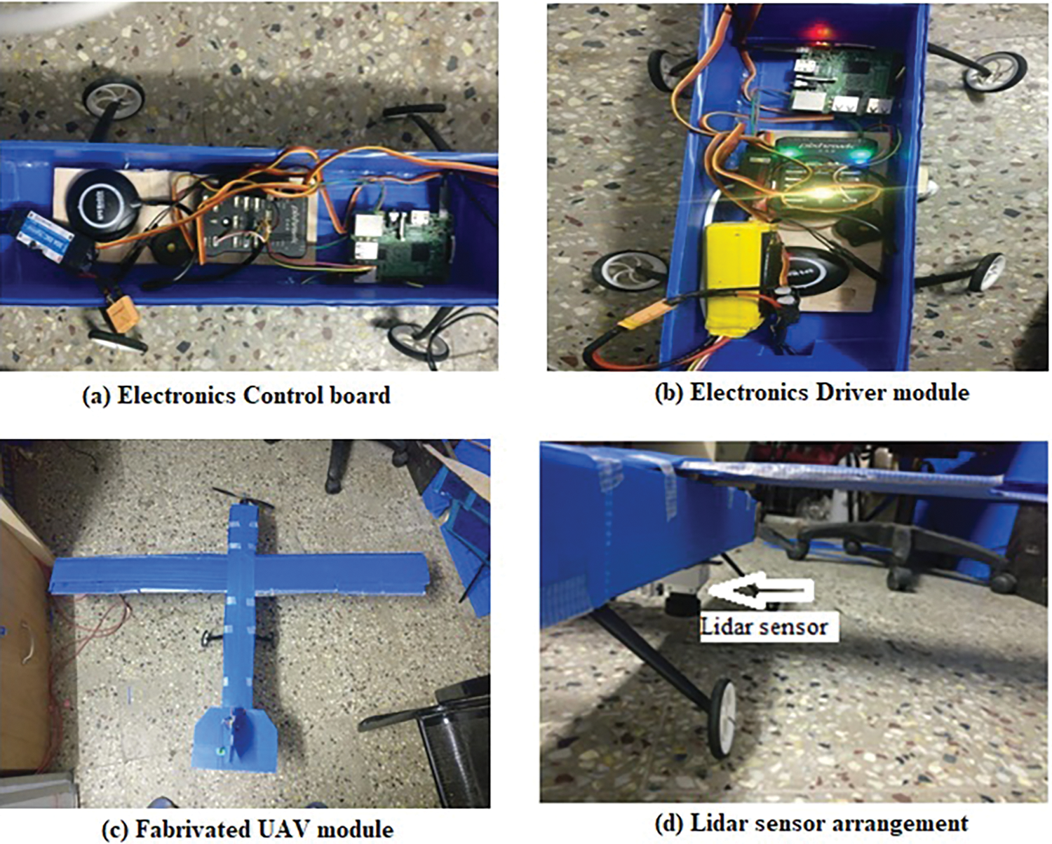
Figure 1: Typical micro UAV exploded view with traditional technology

Different sensors have been used for tracking and fulfilling the flying action of micro aerial vehicles. Some important sensors are IMU, GPS, and I2C barometric Pressure/Altitude/Temperature Sensors are integrated with UAVs. TATTU 8000 mAh 6 s 25c Lipo Battery was used for the long run and lightweight. The increased diameter of the shaft results in less chance of damage to the unfortunate landings and increases the precision of the axial attachment of the propeller–which directly reduces vibration. For higher quality bearings, it is better to terminate the high temperatures. Importantly, the LiDAR sensor with 8 beams is fitted with a downward pointing beam of required tilting angles. This downward fitting covers the area under the UAV which is on the fly.

The primary gun mount’s design allows for two degrees of freedom (DoF). The amount is meant to be solely attachable and removable on the primary gun rail in accordance with system requirements. The gun’s design can be helpful in providing PITCH and YAW action. Every servo motor has its IMU (inertial measurement unit) sensors assigned to it. The secondary cannon has pitch motion from servo 2 and yaw motion from servo 1. The servos are attached to the controller’s digital pins and receive a 5-volt power supply. In this system, a conventional PID controller was used to adopt precise control on the adaptive-loop environment. It regulates the servos loop according to the feedback from the servo motors related to the angular positions. The discrepancy between the process variable and the set point generates the error signal. Additionally, the servo plant is being operated as intended by the PID controller via the error signal. Different mechanical components’ dimensions are chosen based on the design. The primary mount, known as servo mount 1, is composed of 5 mm thick nylon. A pocket measuring 44 mm × 21 mm is crafted in the center of the top of servo mount 1 in order to precisely secure servo motor 1 onto the mount. A force of 6.72 N is being applied to this fabricated CNC machine mount. Fig. 2 displays the CAD model and the mounts’ stress analysis using the Ansys workbench program.

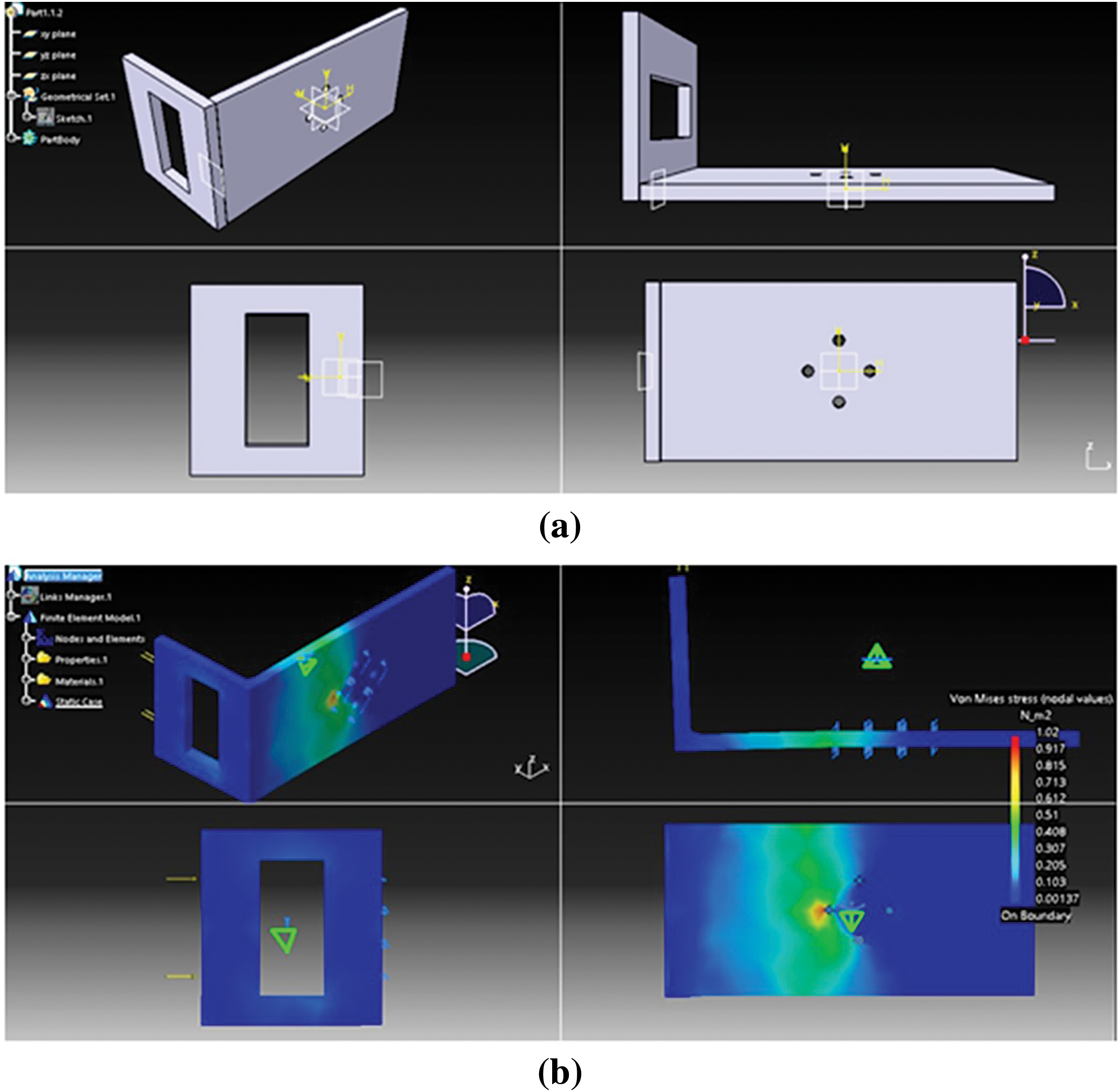
Figure 2: (a) The CAD model (b) Stress analysis of mount 2

3  Mapping Using Eight Beam LiDAR

The Light detection and ranging (LiDAR) module enables developers and integrators to make advanced technologies by integration in detection and ranging systems as shown in Fig. 3. The purpose of the LiDAR module is to easily and rapidly be integrated with various applications. The module can be configured to be used in very simple applications or to perform more complex tasks depending on the hardware and software settings. Distance (or) height can be measured from the base of the standoffs for the LiDAR module. The dashed lines illustrate 1 of the 8 segments and the solid line indicates the distance measured by the module in that segment.

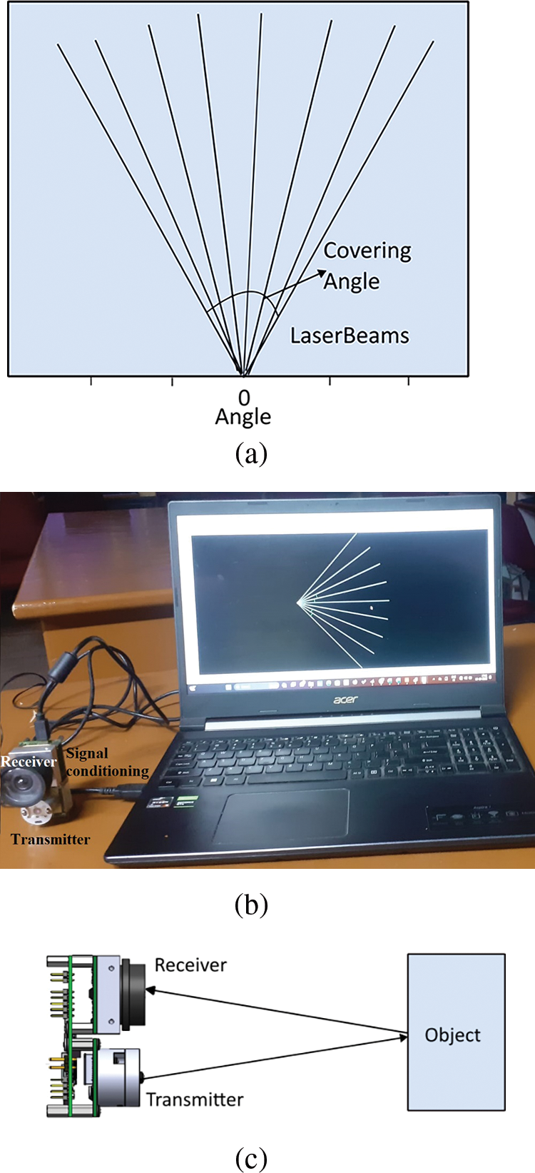
Figure 3: LiDAR arrangement used in the present study (a) 8 beam view (b) Testing of 8 beam LiDAR (c) Measurement of distance/height

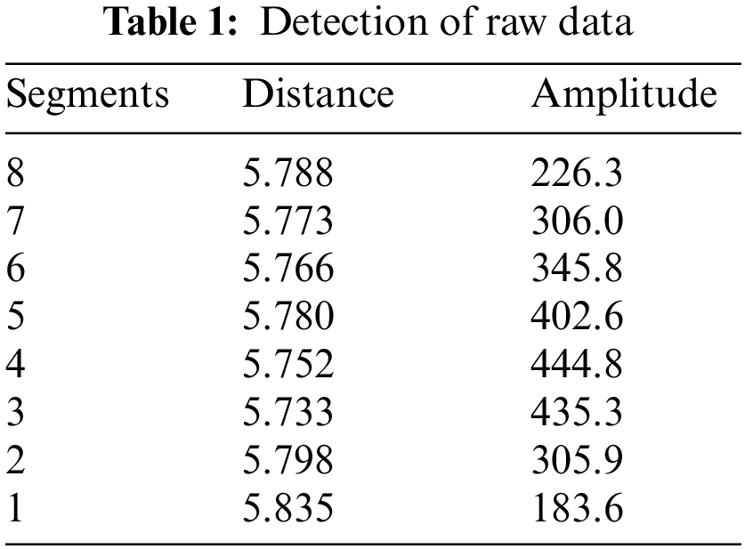
The LiDAR can produce 8 beams with the help of LeddarVu Software 3 (LeddarTech, Canada). The Data displayed in the Raw Detections dialog box allows the user to precisely define the desired detection parameters as shown in Table 1. An object crossing the beam of the module is detected and measured. It is qualified by its distance, segment position, and amplitude. The quantity of light reflected back to the module by the object generates the amplitude. The bigger the reflection, the higher the amplitude will be. The amplitude is expressed in counts. A count is the unit value of the used ADC in the receiver. The fractional count is also used by the accumulation to get more precision. The measurement rate can be calculated using the following Eq. (1):

MR=BARN∗A∗OS(1)

where MR is the measurement rate; N is the Number of segments; A is the Accumulations; and OS is the oversampling. The accumulation and oversampling are the parameters used for improving the measurement process in terms of accuracy and precision. The higher value of accumulation and oversampling enhances the accuracy and precision of measurement and thereby significantly reduces the measurement rate.

3.1 Measurement Using Eight-Beam LiDAR

Three dimensions such as breadth, depth, and height of the object can be measured and measured parameters. Consider an UAV flying from the earth at an altitude ‘a’ meters as shown in Fig. 4. Then, ‘h’ is the average height measured from the UAV in all eight beams. The actual height of the object to be measured and mapped can be calculated by subtracting ‘h’ from ‘a’ and it is indicated in Fig. 4 as ‘g’. Consider an angle of beam deflection from the first laser beam to the last as ‘θ’ and it is a horizontal field of view (FOV). Then, the width (or) breadth can be calculated from average height ‘h’ and horizontal FOV ‘θ’. Then, width (w) can be calculated using the following Eq. (2) as explained in Fig. 5:

w=2b.sin⁡θ2(2)

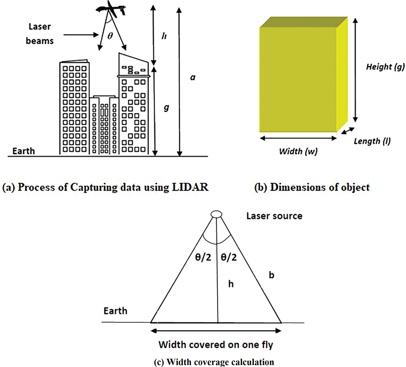
Figure 4: Process of capturing data in the present study

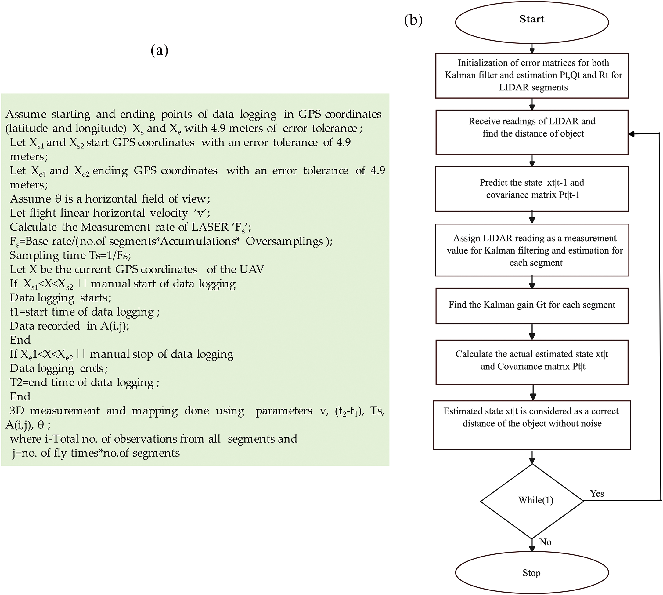
Figure 5: (a) Algorithm of measurement and mapping, (b) Flow diagram of Kalman filter

Assume ‘b’ is approximately equal to the average height ‘h’ as ‘θ’ is small for more resolution. Then, the equation becomes as Eq. (3):

w=2h.sin⁡θ2(3)

The actual length (l) of an observation and length resolution (lr) can be calculated from the UAV parameters and LASER sampling time intervals. Assume ‘v’ is the velocity of the UAV and ‘Ts’ is the sampling time interval of the LASER pulses. Then, the data logging start and end times in the LASER module are t1 and t2. For finding the length of observation in meters and length resolution in the number of samples, the following expressions are used. Eqs. (4) and (5) indicate that the observation length ‘l’ can be mapped using the sample values lr.

l=v∗(t2−t1)(4)

lr=t2−t1Ts(5)

3.2 Algorithm for Mapping of an Object and Noise Cancellation

3.2.1 Algoirthm for Measurement and Mapping

A detailed algorithm for measurement using an 8-beam LiDAR segment is explained as shown in Fig. 5.

3.2.2 Kalman Estimation for 8-Segment LiDAR

Kalman estimation and filtering have been applied at every segment of the LiDAR sensor output to ensure a noise-free and estimated output for missed readings. Kalman is a mathematical procedure for estimating states and offering filtering on white Gaussian noise of LiDAR. There are two important steps in the Klaman estimation as shown in Fig. 5b. In the first step, the state is estimated using previous states along with a state transition matrix, and the state transition matrix for a sensor is unity as one vector value is assumed for sensor output. The estimated state is denoted as x^. Since there is no control input u, and one state measurement, then the remaining parameters Pt, Qt & Rt are state variance, process noise variance, and measurement noise matrices, Gt is assumed to be Kalman Gain. Then, the second step in which the estimated state is corrected using Kalman gain and measurement values. Here, t|t, −1|t−1, t|t−1 are assumed to be current state time, previous state time, and intermediate step transition time. Then, due to the aforementioned assumptions, the Kalman equations are as follows:

{x^t|t−1=x^t−1|t−1Pt|t−1=Pt−1|t−1+Q(6)

{x^t|t=x^t|t−1+Gt(yt−x^t|t−1)Pt|t=(1−Gt)Pt|t−1(7)

Gt=Pt|t−1(Pt|t−1+Rt)−1(8)

4  Results and Discussion

4.1 Intensity of Light in TOF and Type of an Object

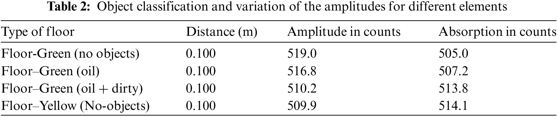
In the present investigation, an endeavor was made to implement mapping of the unknown environment of buildings as described in Fig. 6. An object crossing the beam of the module can be detected and measured. It is measured by its distance, segment position, and amplitude as shown in Table 1. The quantity of light reflected back to the module by the object is measured in the form amplitude. It is usually in counts and it is the unit value ADC in the module receiver. Its count is in fractional to get more precision in the measurement. The larger count value indicates the bigger reflections. However, the reflection depends on the properties of the object such as material, color, etc., and also on the wavelength of the light. The LASER light emits infrared light at a wavelength 905 nm. Then, the variations of the amplitudes for different materials with a fixed distance have been measured and tabulated as shown in Table 2.

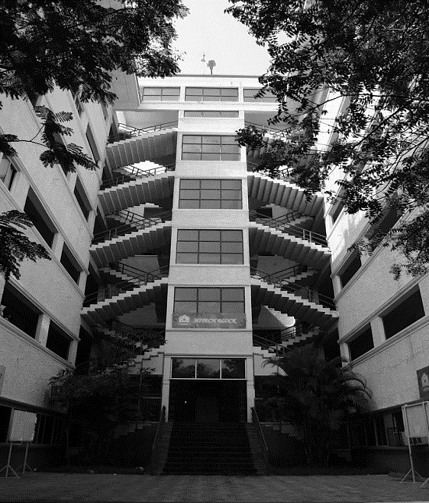
Figure 6: The original view of a building

4.2 Measurement and Mapping Using TOF

The LASER module has been fixed in the slot provided in the UAV. The experiment was conducted with a number of iterations. The data logging and measurement in the LiDAR module is started as per the Algorithm described in Section 3.2. Once the data logging is started, the mapping is also started. If mapping is done on the fly, then it is called as online mapping. It is also possible to perform an offline mode of mapping once data logging is over. The average velocity of the UAV has been fixed at a velocity of 10 m/s. Then, the horizontal field of view can be selected into three categories such as wide (95 degrees), medium (48 degrees), and narrow (16 degrees).

Furthermore, the accuracy of measurement was also noticed by comparing the measured values with the true values of the building with low errors. Even the high accuracy in height measurement is achieved, the length measurement is having error percentage varying from 0% to ±5% of original values. These height measurement values are compared with the conventional camera technique. For camera-based mapping, the technique of stereo vision has been employed for height measurements. The height measurements with a finite number of trials for different UAV flying heights are carried out. These results are plotted as shown in Fig. 7. From the graph, the LiDAR outperforms the conventional camera in height measurement accuracy. Further, the width of coverage is varied by varying parameters multiple beams, height of UAV, and FOV of the LiDAR module. The optimal 8-beam has been chosen as more beams experience latency in side beams over the central beam. Also, it offers a good resolution for measuring the smallest incremental values of 0.5 m as compared with single beam measurement which offers a resolution of 4 m. The optimal 8-beam LiDAR in which low delays in side beams are estimated and approximated using Kalman filter estimation.

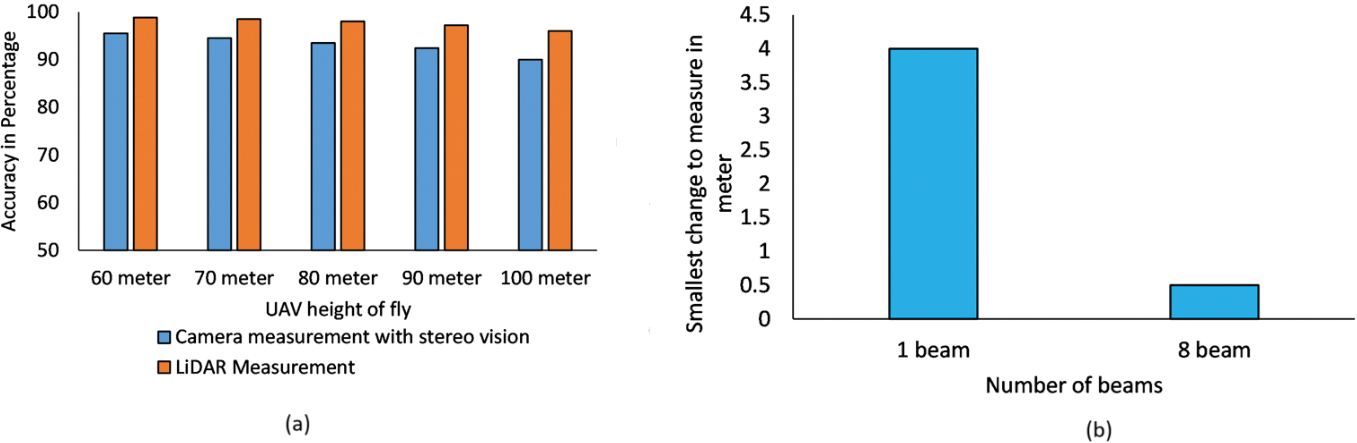
Figure 7: (a) Comparison of height measurement accuracy of LiDAR with a camera with stereo vision measurements. (b) Resolution of 8-beam LiDAR with single-beam LiDAR

The height of the UAV is also adjusted with respect to the FOV to cover the entire area. The wider FOV of UAV takes fewer flies to cover the entire area than the narrower one. However, the wider coverage gives a poor resolution in mapping when an object surface changes as shown in Fig. 8a where the edges are not sharp that much. When the building side wall and openings come, there is no perfect plot due to the non-reachability of multiple reflections at higher altitude measurements. The resolution of plot is also poor on the whole, and especially it is notable at the edges of the building. Resolution has improved by flying at lower heights for mapping at the cost of a greater number of flies as shown in Fig. 8b where the building to be measured is covered on two flies with 16 segments. It is further improved by flying three times to cover the area. Its resolution has been increased, and clear-cutting edges are obtained as shown in Fig. 8c.

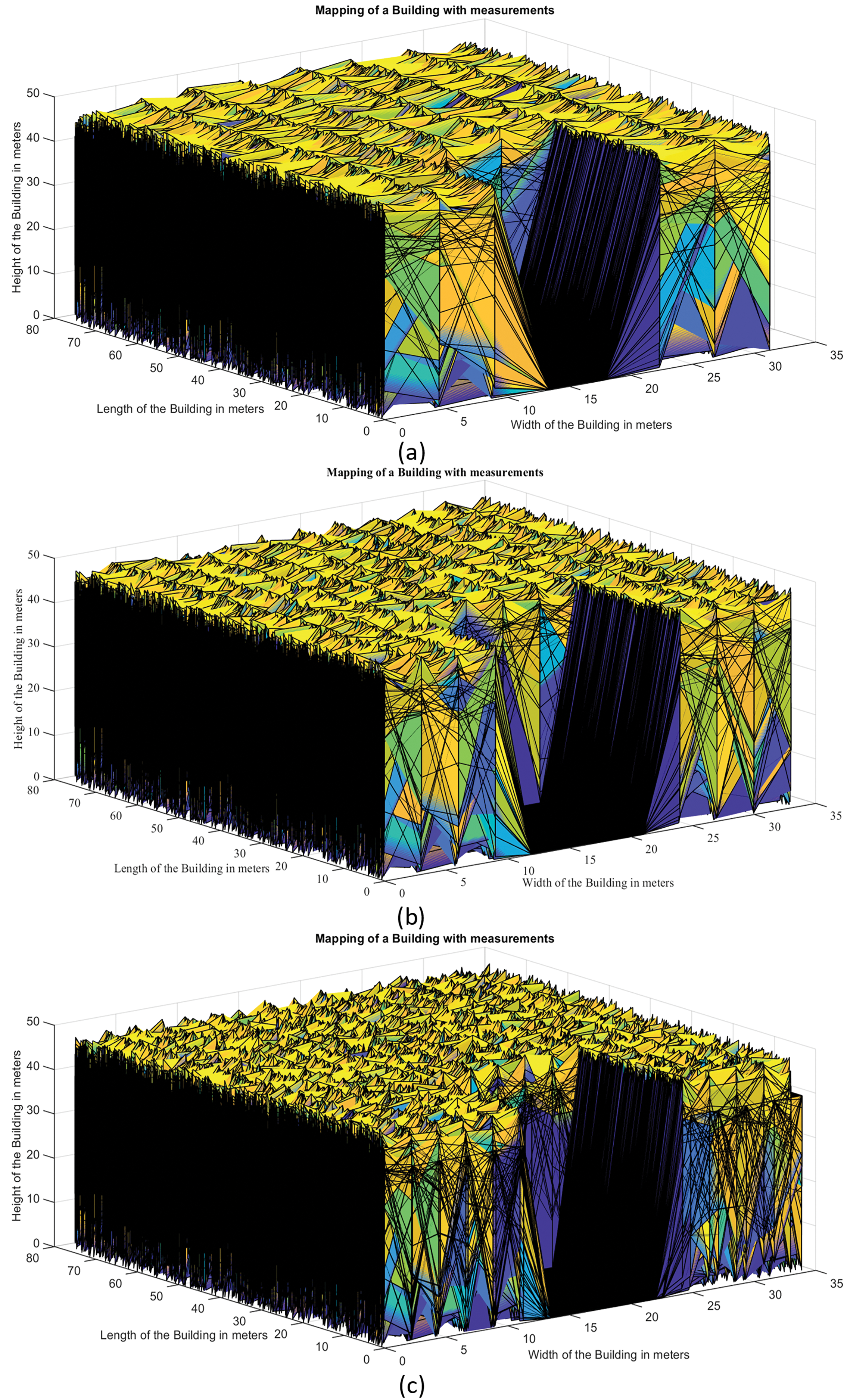
Figure 8: Measurement and mapping of the building in noisy environment without Kalman estimation with v = 10 m/s and observation time (t2 − t1) = 7 s (a) number of fly = 1; number of segments along the width = 8, (b) number of fly = 2; number of segments along width = 16, (c) number of fly = 3; number of segments = 24

However, the number of flies is increased with a reduced FOV to cover the same area. Further, the resolution of mapping has been improved with more number of segments in a narrow FOV. It is evident that the edges of the object have been drawn sharply with larger segments and narrow FOV as shown in Fig. 8. All measurements and mapping have been done in a noisy environment. Moreover, the outputs are taken with noise, and without any estimations.

4.3 Mapping with Kalman Estimation and Filtering

As explained in Section 3.2.2, the Kalman mathematical filtering has been applied on each segment of data with initial assumptions of covariance matrix P as zero and measurement noise R = 10, process noise Q = 1. The missed states during measurement is estimated and the average of white Gaussian noise of measurement is nullified in the Kalman estimation. Then, the actual measurement values have been found using the Kalman estimation in the noisy and missed measured values. The mapping results for different flies are shown in Fig. 9a–c. It is evident that there is a smooth top plot on the mapping.

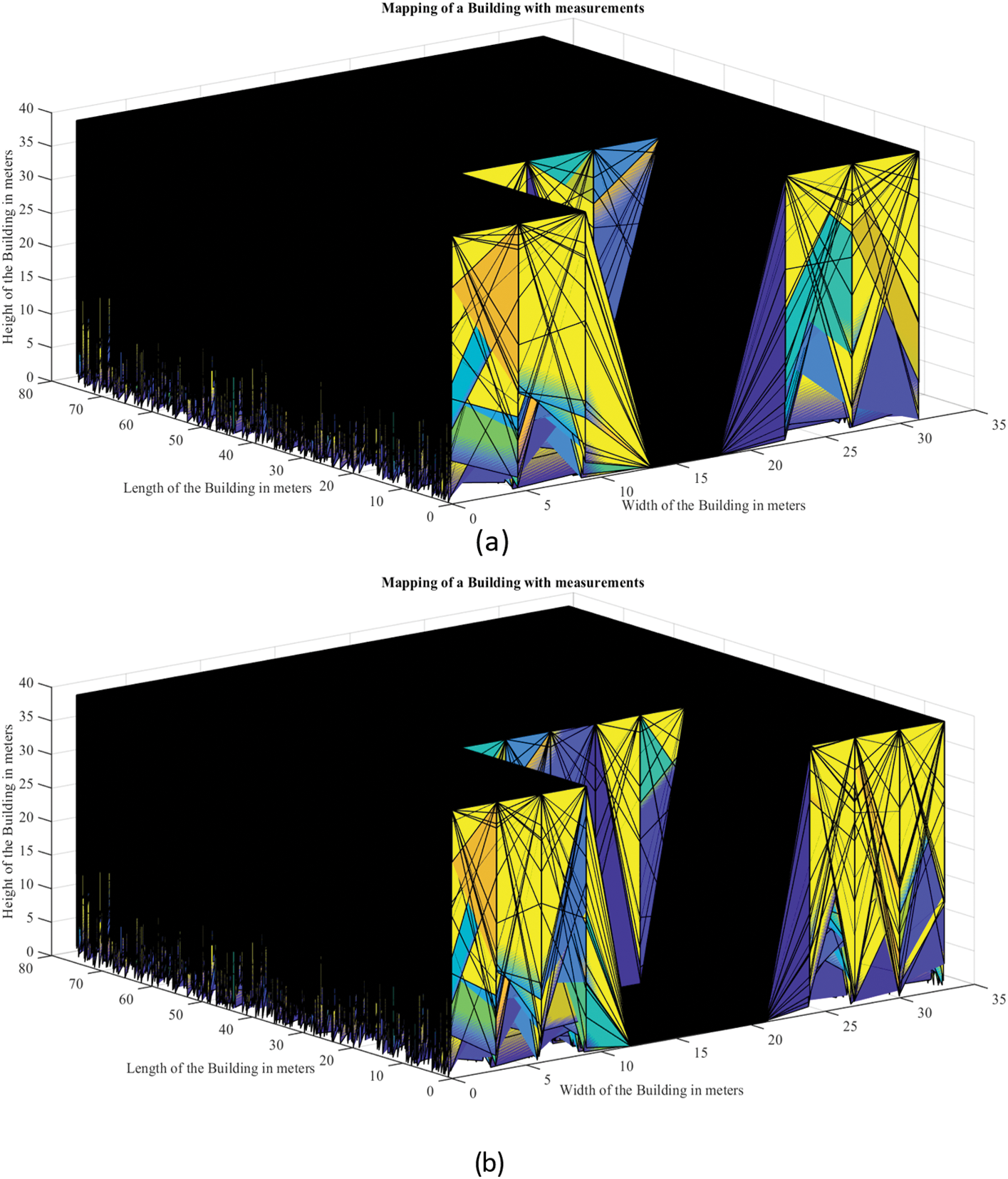
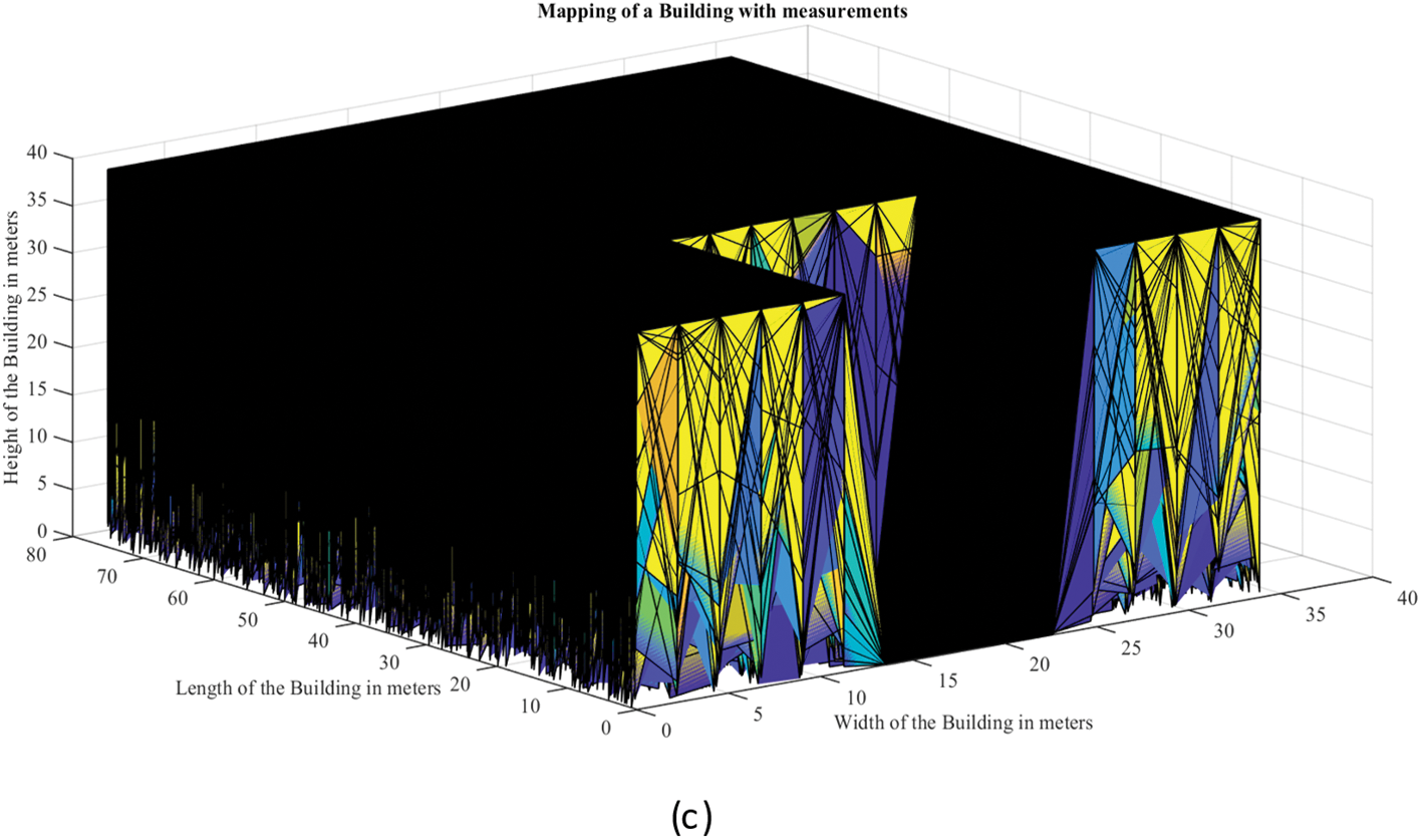
Figure 9: Measurement and mapping of the building in noisy environment with Kalman estimation with v = 10 m/s and observation time (t2 − t1) = 7 s (a) number of fly = 1; number of segments along the width = 8, (b) number of fly = 2; number of segments along width = 16, (c) number of fly = 3; number of segments = 24

5  Conclusions

The proposed approach involves utilizing a parallel 8-beam LIDAR module on the UAV to accurately measure and map larger objects. The process is executed without the utilization of complex software technologies for measurement and mapping. Mapping can be easily performed using both online and offline modes. This technology is well-suited for environments where precise measurement and mapping are crucial, even in the presence of significant noise. The study yielded the following conclusions:

•   The system provides prompt results in comparison to traditional camera-based surveillance, with minimal latency, more accuracy, and the absence of complex algorithms.

•   Due to the absence of complex camera systems and advanced software algorithms, this method proves to be a cost-effective solution.

•   Additionally, an analysis of reflected signals at the same height has been conducted to examine the cleanliness of materials of identical type and color.

•   The system enhances measurement and mapping accuracy in a noisy environment by effectively estimating sensor data and filtering out noise.

This property will prove valuable in the future analysis of the surface of photovoltaic solar panels from a distance, specifically in evaluating their performance.

Further, more beams such as 16 beam LiDAR for higher altitude fly of UAV for covering more area and higher resolution will be studied in the future. The problem of delayed side beams over the central beam will be compensated with a proper design of delay-compensating circuits.

Acknowledgement: The authors extend their appreciation to the King Saud University for funding this work through the Researchers Supporting Project Number (RSPD2024R596), King Saud University, Riyadh, Saudi Arabia.

Funding Statement: This research was funded through the Researchers Supporting Project Number (RSPD2024R596), King Saud University, Riyadh, Saudi Arabia.

Author Contributions: The authors confirm their contribution to the paper as follows: Conceptualization, Mohamed Rabik Mohamed Ismail, Muthuramalingam Thangaraj, Khaja Moiduddin, Zeyad Almutairi, and Mustufa Haider Abidi; methodology, Mohamed Rabik Mohamed Ismail, Muthuramalingam Thangaraj, Khaja Moiduddin, and Mustufa Haider Abidi; software, Muthuramalingam Thangaraj, and Mohamed Rabik Mohamed Ismail; validation, Mohamed Rabik Mohamed Ismail, Muthuramalingam Thangaraj, Khaja Moiduddin, and Mustufa Haider Abidi; formal analysis, Mohamed Rabik Mohamed Ismail, Muthuramalingam Thangaraj, Khaja Moiduddin, and Zeyad Almutairi; investigation, Mohamed Rabik Mohamed Ismail, Muthuramalingam Thangaraj, and Khaja Moiduddin; resources, Muthuramalingam Thangaraj, Khaja Moiduddin, Zeyad Almutairi, and Mohamed Rabik Mohamed Ismail; writing—original draft preparation, Mohamed Rabik Mohamed Ismail, Muthuramalingam Thangaraj, Zeyad Almutairi, Mustufa Haider Abidi, and Khaja Moiduddin; project administration, Muthuramalingam Thangaraj, Khaja Moiduddin, and Zeyad Almutairi; funding acquisition, Muthuramalingam Thangaraj, and Khaja Moiduddin. All authors reviewed the results and approved the final version of the manuscript.

Availability of Data and Materials: This article does not involve data availability and this section is not applicable.

Ethics Approval: Not applicable.

Conflicts of Interest: The authors declare that they have no conflicts of interest to report regarding the present study.

References

1. M. Rabah, A. Rohan, M. Talha, K. H. Nam, and S. H. Kim, “Autonomous vision-based target detection and safe landing for UAV,” Int. J. Control Autom. Syst., vol. 16, no. 6, pp. 3013–3025, 2022. doi: 10.1007/s12555-018-0017-x. [Google Scholar] [CrossRef]

2. M. M. Rabik and T. Muthuramalingam, “Tracking and locking system for shooter with sensory noise cancellation,” IEEE Sens. J., vol. 18, no. 2, pp. 732–735, 2018. doi: 10.1109/JSEN.2017.2772316. [Google Scholar] [CrossRef]

3. M. Rusnák, J. Sládek, A. Kidová, and M. Lehotský, “Template for high-resolution river landscape mapping using UAV technology,” Measurement, vol. 115, no. 1, pp. 139–151, 2018. doi: 10.1016/j.measurement.2017.10.023. [Google Scholar] [CrossRef]

4. H. J. Min, “Generating homogeneous map with targets and paths for coordinated search,” Int. J. Control Autom. Syst., vol. 16, no. 2, pp. 834–843, 2018. doi: 10.1007/s12555-016-0742-y. [Google Scholar] [CrossRef]

5. A. Jawaharlalnehru et al., “Target object detection from Unmanned Aerial Vehicle (UAV) images based on improved YOLO algorithm,” Electronics, vol. 11, no. 1, 2022, Art. no. 2343. doi: 10.3390/electronics11152343. [Google Scholar] [CrossRef]

6. S. Koo, S. Kim, J. Suk, Y. Kim, and J. Shin, “Improvement of shipboard landing performance of fixed-wing UAV using model predictive control,” Int. J. Control Autom. Syst., vol. 16, no. 6, pp. 2697–2708, 2018. doi: 10.1007/s12555-017-0690-1. [Google Scholar] [CrossRef]

7. M. Zeybek and İ. Şanlıoğlu, “Point cloud filtering on UAV based point cloud,” Measurement, vol. 133, no. 1, pp. 99–111, 2019. doi: 10.1016/j.measurement.2018.10.013. [Google Scholar] [CrossRef]

8. E. Akturk and A. O. Altunel, “Accuracy assessment of a low-cost UAV derived digital elevation model (DEM) in a highly broken and vegetated terrain,” Measurement, vol. 136, no. 1, pp. 382–386, 2019. doi: 10.1016/j.measurement.2018.12.101. [Google Scholar] [CrossRef]

9. J. T. Sánchez et al., “Mapping the 3D structure of almond trees using UAV acquired photogrammetric point clouds and object-based image analysis,” Biosyst. Eng., vol. 176, no. 1, pp. 172–184, 2018. doi: 10.1016/j.biosystemseng.2018.10.018. [Google Scholar] [CrossRef]

10. O. Tziavou, S. Pytharouli, and J. Souter, “Unmanned Aerial Vehicle (UAV) based mapping in engineering geological surveys: Considerations for optimum results,” Eng. Geol., vol. 232, no. 1, pp. 12–21, 2018. doi: 10.1016/j.enggeo.2017.11.004. [Google Scholar] [CrossRef]

11. J. J. Sofonia, S. Phinn, C. Roelfsema, F. Kendoul, and Y. Rist, “Modelling the effects of fundamental UAV flight parameters on LiDAR point clouds to facilitate objectives-based planning,” ISPRS J. Photogramm. Remote Sens., vol. 149, no. 1, pp. 105–118, 2019. doi: 10.1016/j.isprsjprs.2019.01.020. [Google Scholar] [CrossRef]

12. D. Huang, Z. Zhang, X. Fang, M. He, H. Lai and B. Mi, “STIF: A spatial-temporal integrated framework for end-to-end micro-UAV trajectory tracking and prediction with 4-D MIMO radar,” IEEE Internet Things. J., vol. 10, no. 21, pp. 18821–18836, 2023. doi: 10.1109/JIOT.2023.3244655. [Google Scholar] [CrossRef]

13. T. F. Villa, F. Gonzalez, B. Miljievic, Z. D. Ristovski, and L. Morawska, “An overview of small unmanned aerial vehicles for air quality measurements: Present applications and future prospectives,” Sensors, vol. 16, no. 21, 2016, Art. no. 1072. doi: 10.3390/s16071072. [Google Scholar] [PubMed] [CrossRef]

14. T. Muthuramalingam and M. M. Rabik, “Sensor integration-based approach for automatic fork lift trucks,” IEEE Sens. J., vol. 18, no. 2, pp. 736–740, 2018. doi: 10.1109/JSEN.2017.2777880. [Google Scholar] [CrossRef]

15. P. M. Carricondo, F. A. Vega, F. C. Ramírez, F. J. Carrascosa, A. G. Ferrer and F. J. Pérez-Porras, “Assessment of UAV-photogrammetric mapping accuracy based on variation of ground control points,” Int. J. Appl. Earth Obs. Geoinform., vol. 72, no. 1, pp. 1–10, 2018. doi: 10.1016/j.jag.2018.05.015. [Google Scholar] [CrossRef]

16. F. A. Vega, F. C. Ramírez, and P. M. Carricondo, “Assessment of photogrammetric mapping accuracy based on variation ground control points number using unmanned aerial vehicle,” Measurement, vol. 98, no. 1, pp. 221–227, 2017. doi: 10.1016/j.measurement.2016.12.002. [Google Scholar] [CrossRef]

17. E. Kaartinen, K. Dunphy, and A. Sadhu, “LiDAR-based structural health monitoring: Applications in civil infrastructure systems,” Sensors, vol. 22, no. 12, 2022, Art. no. 4610. doi: 10.3390/s22124610. [Google Scholar] [PubMed] [CrossRef]

18. C. Song, Z. Chen, K. Wang, H. Luo, and J. C. P. Cheng, “BIM-supported scan and flight planning for fully autonomous LiDAR-carrying UAVs,” Autom. Constr., vol. 142, no. 1, 2022, Art. no. 104533. doi: 10.1016/j.autcon.2022.104533. [Google Scholar] [CrossRef]

19. W. Xu and F. Zhang, “FAST-LIO: A fast, robust LiDAR-inertial odometry package by tightly-coupled iterated Kalman filter,” IEEE Robot. Automat. Lett., vol. 6, no. 1, pp. 3317–3324, 2021. doi: 10.1109/LRA.2021.3064227. [Google Scholar] [CrossRef]

20. C. Gao et al., “A UAV-based explore-then-exploit system for autonomous indoor facility inspection and scene reconstruction,” Autom. Constr., vol. 148, no. 1, 2023, Art. no. 104753. doi: 10.1016/j.autcon.2023.104753. [Google Scholar] [CrossRef]

21. N. Bolourian and A. Hammad, “Lidar-equipped UAV path planning considering potential locations of defects for bridge inspection,” Autom. Constr., vol. 117, no. 1, 2017, Art. no. 103250. doi: 10.1016/j.autcon.2020.103250. [Google Scholar] [CrossRef]

22. Y. C. Lin et al., “Evaluation of UAV LiDAR for mapping coastal environments,” Remote Sens., vol. 11, no. 1, 2019, Art. no. 2893. doi: 10.3390/rs11242893. [Google Scholar] [CrossRef]

23. M. P. Christiansen, M. S. Laursen, R. N. Jørgensen, S. Skovsen, and R. Gislum, “Designing and testing a UAV mapping system for agricultural field surveying,” Sensors, vol. 17, no. 1, 2017, Art. no. 2703. doi: 10.3390/s17122703. [Google Scholar] [PubMed] [CrossRef]

24. G. Rossi, L. Tanteri, V. Tofani, P. Vannocci, S. Moretti and N. Casagli, “Multitemporal UAV surveys for landslide mapping and characterization,” Landslides, vol. 15, no. 1, pp. 1045–1052, 2018. doi: 10.1007/s10346-018-0978-0. [Google Scholar] [CrossRef]

25. T. Kim and T. H. Park, “Extended Kalman Filter (EKF) design for vehicle position tracking using reliability function of Radar and Lidar,” Sensors, vol. 20, no. 15, 2020, Art. no. 4126. doi: 10.3390/s20154126. [Google Scholar] [PubMed] [CrossRef]

26. Y. W. Hsu, Y. H. Lai, K. Q. Zhong, T. K. Yin, and J. W. Perng, “Developing an on-road object detection system using monovision and Radar fusion,” Energies, vol. 13, no. 1, 2020, Art. no. 116. doi: 10.3390/en13010116. [Google Scholar] [CrossRef]

27. W. H. Lio, G. C. Larsen, and G. R. Thorsen, “Dynamic wake tracking using a cost-effective LiDAR and Kalman filtering: Design, simulation and full-scale validation,” Renew. Energy, vol. 172, no. 1, pp. 1073–1086, 2021. doi: 10.1016/j.renene.2021.03.081. [Google Scholar] [CrossRef]

28. T. -L. Kim, J. -S. Lee, and T. -H. Park, “Fusing lidar, radar, and camera using extended Kalman filter for estimating the forward position of vehicles,” in 2019 IEEE Int. Conf. Cybern. Intell. Syst. (CIS) IEEE Conf. Robot., Autom. Mechatron. (RAM), Bangkok, Thailand, 2019, pp. 374–379. doi: 10.1109/CIS-RAM47153.2019.9095859. [Google Scholar] [CrossRef]

29. M. B. Maru, D. Lee, G. Cha, and S. Park, “Beam deflection monitoring based on a genetic algorithm using Lidar data,” Sensors, vol. 20, no. 7, 2020, Art. no. 2144. doi: 10.3390/s20072144. [Google Scholar] [PubMed] [CrossRef]