A Low Complexity ML-Based Methods for Malware Classification

1  Introduction

The security and integrity of computer systems [1–3] and networks are seriously threatened by the spread of malware or malicious software. Malware can carry out various nefarious tasks, including financial fraud, network disruption, system intrusion, and data theft. Effective detection and mitigation approaches are becoming increasingly important as malware’s sophistication and complexity continue to grow. Malicious software is classified as worms, viruses, trojan horses, rootkits, backdoors, spyware, logic bombs, adware, and ransomware based on its behaviour and execution. Hackers target computer systems for several objectives, such as destroying resources, gaining financial gain, stealing private information, using resources, and disrupting system functions [4,5].

Despite recent advances in malware classification, researchers continue to encounter several challenges. Some of the current obstacles in the field include:

1.    Advanced Malware: Malware is growing more complex, with attackers continuously devising new ways to avoid detection. As a result, it is difficult to ssrecognize and categorise new malware effectively.

2.    Big Data: The number of malware samples created continually rises, creating big data difficulties that need significant processing and storage capabilities. Furthermore, the data quality varies greatly, making it difficult to extract valuable information.

3.    Adversary Evasion tactics: Attackers frequently utilise evasion tactics to avoid detection systems, such as polymorphic code or malware encryption. These methods might make it challenging to identify and categorise malware correctly.

4.    Privacy risks: Malware classification necessitates access to sensitive data, including personal or secret information, raising privacy risks. Researchers must balance the requirement for data access with privacy considerations, which may limit access to specific datasets.

Researchers are adopting sophisticated Machine Learning and Deep Learning algorithms, hybrid models, and improved feature engineering approaches to solve these issues. Furthermore, creating new techniques for detecting emerging malware and increasing model generalisation might help progress the area of malware classification. Interpolation is particularly utilised in the field for the first time to overcome some annoying problems in this field. Interpolation increases the accuracy of malware classification and categorisation in various ways. When dealing with malware samples, the data is often represented in distinct feature spaces, making direct comparisons problematic. Interpolation bridges the gap between distinct sets of features, allowing the model to collect more helpful information about the samples and, hence, improve classification accuracy.

Interpolation can also help overcome challenges with missing values and outliers, typical in malware classification datasets. By filling these gaps, the suggested technique can provide a more comprehensive dataset, lowering noise or bias in the data and thereby boosting classification accuracy. Furthermore, interpolation approaches prevent overfitting and increase model generalisation, allowing for more accurate classification of fresh malware samples. Finally, interpolation increases malware classification accuracy by closing feature space gaps, filling in missing data, lowering outliers, and boosting model generalisation.

When it comes to detecting malware, there are three main approaches that security experts generally use-Signature-based, Anomaly-based, and Specification-based detection. Also, within those broad categories, they can further refine the techniques into static, dynamic, and hybrid methods [6,7].

In this research work, we provide a revolutionary real-time malware detection method that combines state-of-the-art Machine Learning techniques with an inventive interpolation-based feature dimensionality reduction strategy. The main contributions of this paper are threefold:

1.    We introduce a novel interpolation-based technique that reduces the dimensionality of the feature space while preserving the most informative features. This approach enables the detection of complex patterns and relationships in the data, improving malware detection accuracy.

2.    We carefully designed our proposed technique to operate in real-time, enabling the detection of malware in a timely and efficient manner. This is particularly important in today’s fast-paced digital landscape, where rapid detection and response are critical to preventing malware outbreaks.

3.    We conducted an empirical study to evaluate the effectiveness of ML-based models and identify challenges for future research. Our solution demonstrates how Machine Learning and interpolation-based feature dimensionality reduction work together to detect real-time malware with excellent accuracy and low overhead costs.

The rest of the paper is organised as follows. Section 2 provides a literature review of existing malware classification techniques. An overview of the proposed Interpolation-based Feature Dimensionality Reduction Technique (IFDRT) combined with optimised ML-based classifiers is provided in Section 3. Section 4 exhibits the results of experiments evaluating the framework’s suitability for malware classification, and in the end, Section 5 concludes the paper.

2  Literature Review

Wang et al. [8] created PAYL, a tool that determines the anticipated payload for each service in a system. They generated a byte frequency distribution and a centroid model for each host’s services. The detector compares incoming payloads to the centroid model and calculates the Mahalanobis distance. The approach was tested on 1999 MIT Lincoln Labs data and detected 57 out of 201 attempts, resulting in low detection rate of around 60%. Taylor et al. [9] presented a low-cost approach to network intrusion detection using anomaly-based detection. The authors propose a system called Nate (Network Analysis of Anomalous Traffic Events), which uses statistical analysis and Machine Learning techniques to identify anomalous network traffic. One major drawback of Nate’s is limited scalability since its performance may suffer as the volume of network traffic rises, making it less useful in high-traffic networks.

Boldt et al. [10] employed computer forensic approaches to detect Privacy-Invasive Software (PIS), such as adware and spyware, which are commonly detected in file-sharing software. The authors propose a framework for detecting and analysing spyware using digital forensic techniques, including file system analysis, network traffic analysis, and memory analysis. They discovered that Ad-Aware generates both false positives and false negatives. Sekar et al. [11] proposed a Finite State Automata (FSA) for anomaly detectionto model the behavior of programs and detect anomalies. The approach is based on the idea that normal program behaviour can be modeled using a finite state automaton, and deviations from this model can be used to detect anomalies. The approach may generate a high number of false positive alerts, which can lead to alert fatigue and decreased effectiveness.

Hofmeyr et al. [12] developed a method for detecting malicious system call sequences. They constructed profiles representing regular system service activity and used the Hamming distance to assess similarity. A threshold was established to detect unusual processes. The approach was successful in detecting intrusions that attempted to exploit UNIX applications. The approach is limited to detecting anomalies in system call sequences and may be ineffective in detecting other attack types. Li et al. [13] presented a novel approach to identifying file types using n-gram analysis. They create models based on the system’s expected file types, assuming that benign files have predictable byte compositions. Any file that deviates considerably from the model is flagged as suspicious and evaluated by a system to determine its maliciousness. This approach requires significant computational resources to analyse the frequency of n-grams in large files.

Forrest et al.’s [14] Anomaly-based approach seeks to identify changes to protected data, however, it cannot detect the removal of items from the collection. The authors suggest an effective approximation of “Other”, however, this incurs processing expenses. The authors offer user-defined matching, such as comparing ten-character strings. Tests on the TIMID virus demonstrated that as the number of detectors increased, so did the detection rate. The approach is often unsuitable for real-world detection tools. Ko et al. [15] created a specification-based technique for identifying malicious behavior in distributed systems. They developed a Distributed Program Execution Monitor (DPEM) that parses audit trails in real time. The system uses formal specifications of program behavior to monitor and detect deviations from expected behavior. The approach may not be scalable to large and complex distributed systems, where the number of programs and specifications can be very large. Xiong [16] presented a novel approach to email virus detection and control called Attachment Chain Tracing (ACT). The approach involves tracing the attachment chain of an email to identify and block malicious attachments. The approach is limited to detecting email viruses and may not be effective against other types of malware.

Debbabi et al. [17] presented a novel approach to securing Commercial-Off-The-Shelf (COTS) software components. The authors propose a self-certification mechanism that allows COTS vendors to certify the security properties of their components. The approach relies on the honesty and integrity of COTS vendors, which may not always be the case. Moreover, it assumes that security properties can be formally specified, which may not be possible for complex systems. Filiol [18] proposed a novel scheme to malware pattern scanning that is secure against black-box analysis. Black-box analysis refers to the process of reverse-engineering a malware detection system to identify its patterns and evade detection. The author’s scheme uses a combination of techniques to make malware pattern scanning more secure, including polymorphic patterns, obfuscated patterns, pattern fragmentation, and pattern encryption. Unfortunately, the scheme may introduce significant complexity, making it difficult to implement and maintain.

Many other researchers applied ML-based techniques in Malware classification and categorisation. Another approach is to convert malware binaries to grayscale or RGB pictures and categorise them. Baptista et al. [19] created a deep learning-based method for identifying malware by transforming binary files into RGB images. In [20–23], the authors used a Convolutional Neural Network (CNN) to identify malware by converting data to greyscale and colour pictures. Image-based malware analysis approaches may also be used to detect Android malware. Anyway, most image-based malware analysis methods may not be ideal for devices with low resources requiring real-time security.

Nasser et al. [24] introduced DL-AMDet, a deep learning-based architecture for detecting malware in Android applications. The DL-AMDet architecture consists of two main detection models. Static Analysis: uses CNN-BiLSTM to detect malware based on static features like API calls and system calls, while Dynamic Analysis: utilises deep autoencoders as an anomaly detection model based on dynamic features. In this combination, very high detection rates can be achieved, but it still suffers from the time-consuming nature of dynamic feature extraction and the complexity of real-time analysis. Hao et al. [25] created a CNN-based feature extraction and channel-attention module to reduce information loss during feature picture synthesis for malware samples. Deep learning architectures, such as deep belief networks and transformer-based classifiers, were utilised to classify PE malware [26]. Anyway, most image-based malware analysis approaches may not be ideal for low-resource systems requiring real-time security.

Despite numerous research efforts on malware analysis, few consider the memory overhead and computational complexity of classification models. Few modern techniques aim to make detection and classification tasks lightweight, resulting in models suitable for mobile and embedded devices. Some techniques, such as [27], stress the lightness of feature vector size and execution durations. Currently, no malware analysis research has demonstrated how lightweight detection and classification models are in terms of memory usage, model training and prediction time overhead. This paper attempts to bridge this gap by presenting lightweight models for resource-constrained devices areappropriate for real-time IOT device operations.

3  Materials and Methods

In this research, we employed Machine Learning to classify malware from the BODMAS [28] dataset available at https://whyisyoung.github.io/BODMAS/ (accessed on 1 June 2024). The models we applied are Extra Trees Classifier (ETC), k-Nearest Neighbor (k-NN), Bagging Classifier (BC), Random Forest (RF), XGBoost (XGB), AdaBoost (ABC) and Light Gradient Boosting Machine (LGBM). Before that, we consider performing some necessary preprocessing and dimensionality reduction on the dataset features, followed by creating, training, and improving the final ML-models. We outline our suggested method’s phases in greater detail in the following subsections.

3.1 BODMAS Dataset

The BODMAS Malware Dataset is used to undertake extensive assessments of the effectiveness and efficiency of the suggested ML-Based Malware Classification Techniques. The BODMAS dataset comprises 57,293 malware samples and 77,142 benign samples gathered between August 2019 and September 2020, with properly curated family information (581 families). Each sample is represented by a 2381 feature vector, which includes the label (benign or malware) and, if malicious, the malware family. It is intended to improve ML-based malware analysis and temporal analysis of Portable Executable (PE) malware. Fig. 1 shows the Malware Counts by Family Distribution.

Figure 1: Malware counts by family

3.2 Dimensionality Reduction

Dimensionality reduction is a Machine Learning approach that reduces the number of features (variables) in a dataset while retaining the most significant information. Consider a dataset with hundreds or even thousands of characteristics for each data point. This high dimensionality might pose challenges, such as Curse of dimensionality, Increased computational cost, and Overfitting.

3.2.1 Importance of Dimensionality Reduction

Dimensionality reduction addresses the issues mentioned above by translating the data into a lower-dimensional space while preserving the most relevant changes. This has various benefits:

•   Improved model performance: By selecting just important features, we may direct the model’s attention to the most informative data sections, resulting in better prediction performance.

•   Reduced overfitting: High-dimensional datasets can result in overfitting, in which the model learns noise or irrelevant patterns from the input. Dimensionality reduction reduces dataset complexity, mitigates overfitting, and improves the generalisation performance of ML-models.

•   Efficient computation: Additional computer resources and time are required to train ML-based models with high-dimensional datasets. Reduced dataset dimensionality lowers the computing cost of training and inference, allowing for quicker model creation and deployment.

•   Enhanced data visualisation: Lower-dimensional data is easier to display, resulting in a better grasp of feature correlations.

In Machine Learning literature, there are many feature extraction techniques, including Principal Component Analysis (PCA), Factor Analysis (FA), Truncated Singular Value Decomposition (tSVD), and many more techniques. In this work, we propose a new novel dimensionality reduction technique to enhance the Machine Learning process; we call it the Interpolation-based Feature Dimensionality Reduction Technique, abbreviated (IFDRT). The proposed technique IFDRT is based on the idea of Interpolation borrowed from the Image Processing field. Interpolation is a mathematical technique for estimating values based on existing data points. It entails creating new data points within a finite collection of known data points. Interpolation is widely used in various disciplines, including mathematics, computer science, engineering, and data analysis, for tasks such as data smoothing, curve fitting, and function approximation. Here’s a breakdown of interpolation concepts:

•   Known data points: These are the current values for our function or data. In our case, these are the feature values.

•   Unknown data points: These are the points where we want to estimate the value of the function, i.e., the reduced features.

•   Interpolation method: This is the mathematical method or procedure used to estimate the value of an unknown point based on the known points around it. Distinct interpolation methods have distinct advantages and disadvantages.

There are several sorts of interpolation methods, each having pros and disadvantages. Some standard methods include:

•   Linear interpolation: Linear interpolation connects two neighbouring data points with a straight line and estimates values at intermediate places along the line. It is simple and computationally efficient, but it may not reflect the underlying trends in the data.

•   Polynomial interpolation: Polynomial interpolation involves fitting a polynomial curve to the data points and using that curve to estimate values at intermediate locations. It gives a more flexible and precise representation of the data, although it may be prone to overfitting.

•   Spline interpolation: Spline interpolation splits the dataset into segments and assigns polynomial curves (often cubic) to each. It performs a smooth and continuous data interpolation, preventing sudden shifts in the interpolated curve.

In this work, a novel feature dimensionality reduction technique is proposed. The feature vector is locally fitted with a suitable mathematical model that best represents the dataset dynamics; then this model is utilised to build a function using interpolation. Then, the interpolated function will be used to find corresponding values of new feature points that will be considered as the new reduced feature points later on. More details about IFDRT will be outlined in subsequent section.

3.3 Types of Dimensionality Reduction

3.3.1 Interpolation-Based Feature Dimensionality Reduction Technique (IFDRT)

The proposed IFDRT is based on the idea of local modelling of feature data points, i.e., the same feature vector is projected into another hyperplane by finding a suitable mapping function f( ) which can be best fit with the features vector ξi. Then, Interpolation is used to create the fitted projection function that will be used to predict new reduced hyperplane items υj, where j << i.

The steps of performing IFDRT are as follows:

1.    For each dataset sample ξi, perform Min-Max normalisation of features to a specific range, which can be helpful for data visualisation or interpreting model coefficients and reduces the variance of features.

2.    Sort the features ξi of each data sample in an ascending order manner.

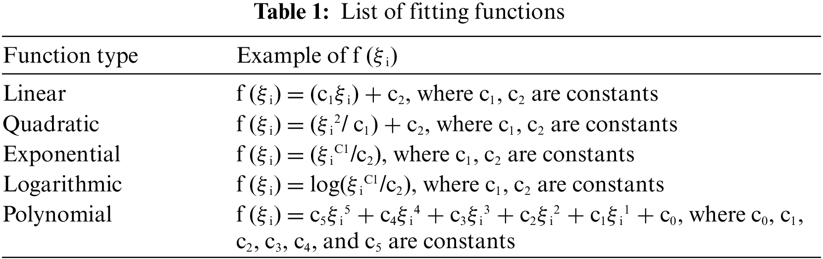
3.    Suggest a fitting function f (ξi) that best matches the data sample distribution. The fitting function can be any function, e.g., linear, quadratic, cubic, polynomial, etc. Refer to Table 1 for some examples of fitting function f( ).

4.    Apply linear, polynomial, or spline interpolation on (ξi, f (ξi)). This will help in producing a fitted function f (ξi).

5.    Generate equally spaced data points ϒj-where j represents the number of components that constitute the reduced feature dimension-in the same range of the data samples generated in Step (1).

6.    Apply f (ϒj), producing a set of newly generated reduced features set υj.

Once IFDRT steps generate a new set of υj, it shall undergo the ML-modeling steps using any Machine Learning algorithm as depicted in Fig. 2. When an objective target criterion is achieved, such as an F1 score greater than 0.98, the IFDRT process is terminated. If the target is not achieved, we can change fitting function f( ) until we find a suitable one and the target criterion is achieved.

Figure 2: Block diagram of IFDRT process

The key advantages of IFDRT include:

1.    Efficient Dimensionality Reduction: By leveraging interpolation techniques, IFDRT can effectively reduce the dimensionality of high-dimensional data while preserving the underlying structure and relationships.

2.    Interpretability: The selected features in IFDRT can provide insights into the most important characteristics of the data, making the dimensionality reduction process more interpretable.

3.    Robustness: IFDRT is generally robust to noise and outliers in the data, as the interpolation step can smooth out these effects.

The steps of IFDRT are depicted in Fig. 2.

A list of alternative fitting functions is shown in Table 1.

Keep in mind that any function can be considered. This empowers the proposed method and benefits in dealing with many statistical attributes specifically related to the underlying dataset. In BODMAS dataset, we the applied Quadratic function to map f (ξi) to υj with ϒj n_components.

After applting IFDRT (two components) on BODMAS dataset, we can see in Fig. 3, the Malware instances are concentrated in a narrow channel after being reduced using IFDRT. Thus, it can be easily identified and learned using high accuracy ML-models. This implies a good behavior of ML-models can be achieved. This will be indicated in next sections during model training and testing experimentation.

Figure 3: Dimensionality reduction using IFDRT (two components) on BODMAS dataset

3.3.2 Principal Component Analysis (PCA)

Principal Component Analysis (PCA) [29] is a dimensionality reduction approach for converting high-dimensional data to a lower-dimensional representation. It finds patterns and correlations in data by projecting them onto a new collection of orthogonal characteristics known as principal components. By keeping only the top k components, PCA decreases data dimensionality, improves data presentation, and improves Machine Learning model performance by minimising noise and the curse of dimensionality.

Fig. 4 shows that the two classes, benign and malware, cannot be easily separable when projected to a two-dimensional space using PCA. Another observation could be that the benign class is more spread out than the malware class. Thus, another dimensionality reduction should be tested. It may require more than two components to interpret the relationships between variables easily.

Figure 4: Dimensionality reduction using PCA (two components) on BODMAS dataset

3.3.3 Factor Analysis (FA)

Principal Factor Analysis (FA) [30] is a statistical method for decreasing the dimensionality of a dataset by identifying latent variables (factors) that explain the observable variables. Unlike PCA, FA assumes some error in the measured variables and seeks to capture the common variation shared by the variables but not caused by measurement error. The most significant disadvantage of employing FA is that selecting the number of variables is not always straightforward. There are various ways to calculate the number of components, however they might be subjective or arbitrary. Furthermore, FA presupposes that the connection between variables and factors is linear, which may not always be true in real-world data. Finally, interpreting the factors might be problematic, especially when complicated variable loadings are across numerous components.

After applying FA on BODMAS dataset with two FA’s, the results are depicted in Fig. 5. We can see that the two FA components have not accurately captured the variation driven by dataset feature variables. It’s easily noticeable that both Benign and Malware classes are sparsed, and no distinct clusters are found. Thus, we conclude that the FA technique may not be the best suitable approach for BODMAS dataset.

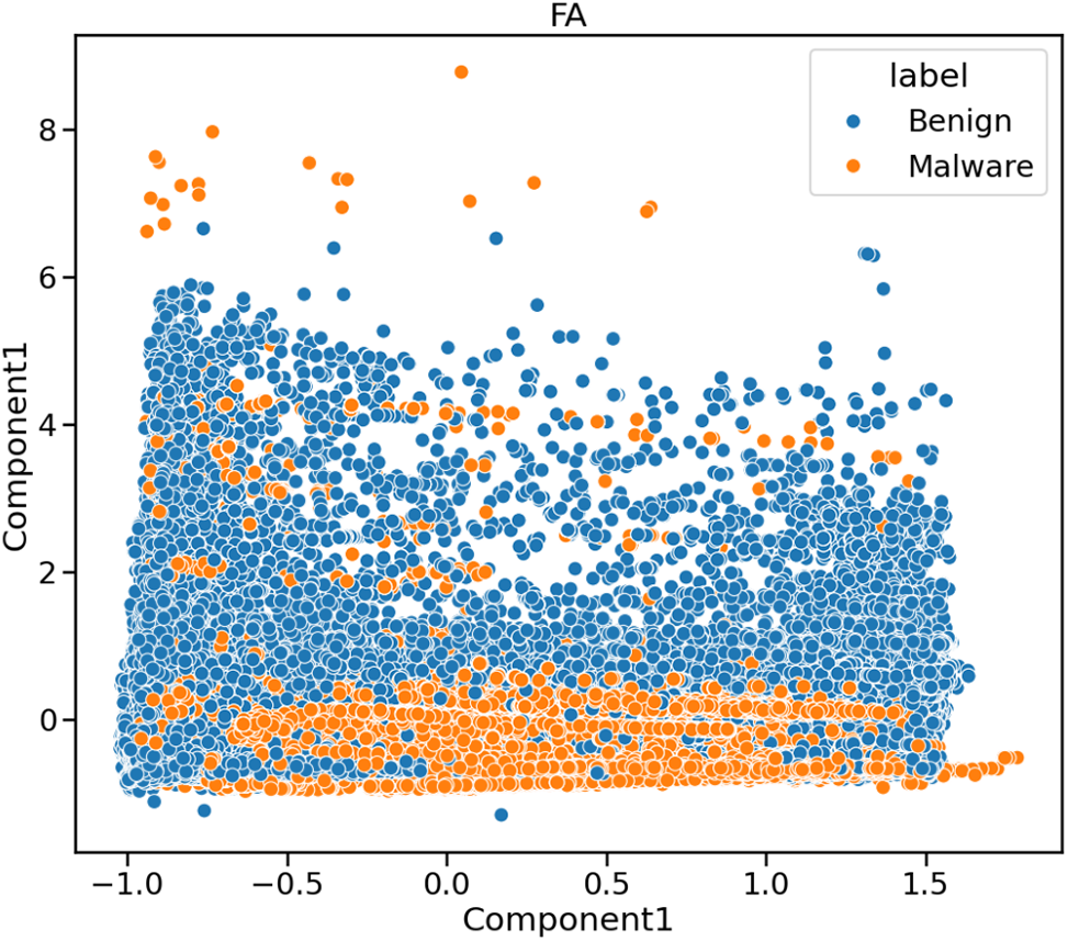
Figure 5: Dimensionality reduction using FA (two components) on BODMAS dataset

3.3.4 Truncated Singular Value Decomposition (tSVD)

Truncated Singular Value Decomposition (tSVD) [31] is a matrix factorisation technique used to reduce a dataset’s dimensionality. SVD decomposes a matrix into three matrices: U, S, and V. U represents the left singular vectors, S represents the singular values, and V represents the suitable singular vectors. Truncated SVD is a version of SVD in which the smallest singular values are dropped, resulting in a matrix with reduced dimensionality. The biggest downside of shortened SVD is that it may lose some information by removing the lowest single values. This can cause a decrease of accuracy in some types of data. Furthermore, shortened SVD is computationally costly and may not be practical for big datasets. Finally, interpreting the resultant shortened SVD matrix might be problematic since each variable’s contribution to the reduced-dimensional representation is unclear.

After applying tSVD on BODMAS dataset with two components, the results are shown in Fig. 6. It shows that the Malware points may be non-linearly split and segregated among the Benign samples. However, a more non-linear method is required to complete the classification task while retaining stronger class segregation. It may necessitate more components to interpret the non-linearity between variables better.

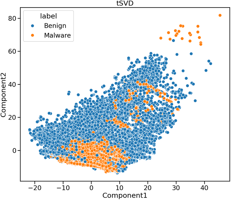
Figure 6: Dimensionality reduction using tSVD (two components) on BODMAS dataset

3.4 Machine Learning

Machine Learning is a branch of artificial intelligence that focuses on creating algorithms and models that allow computers to learn and make predictions or judgments without being explicitly programmed [32,33]. Large datasets are analysed and interpreted using statistical techniques and computer-based models. Machine Learning has gained popularity and has been used in various fields, including computer vision, natural language processing, and data mining. One of the fundamental concepts in Machine Learning is using training data to create models capable of generalising and making accurate predictions on previously unknown data. This approach includes optimising model parameters using techniques like gradient descent or stochastic gradient descent. The unique issue and data characteristics determine the learning method and model architecture used. Several researchers have helped progress Machine Learning. For example, Domingos’ [34] delves into the practical elements of Machine Learning, such as the value of feature engineering and the bias-variance tradeoff. Another work by He et al. [35] introduced residual networks and shows its efficacy in picture classification tasks.

Machine Learning techniques, such as neural networks, decision trees, and support vector machines, identify complex patterns and correlations from massive datasets, providing insights and predictions that standard statistical approaches may fail to detect. Those methods have found significant use in various fields, including healthcare and finance, as well as natural language processing and computer vision. Additionally, Machine Learning is essential to malware detection because it offers quick and easy ways to recognise and categorise harmful software. Due to the significant advances in Machine Learning, it is now simpler to create lightweight algorithms that can identify malware and take immediate action to protect systems and data. Machine Learning empowers malware detection systems to analyse and classify malware samples effectively, adapt to evolving threats, and provide timely protection against cyber-attacks. By leveraging Machine Learning techniques, security practitioners can enhance their cybersecurity posture and safeguard digital assets against various malware threats.

In this work, we applied a variety of feature directionality reduction techniques-illustrated above-on BODMAS to examine the efficacy and efficiency of Machine Learning in creating new, potent frameworks for malware detection. We then trained the system using well-known Machine Learning algorithms, such as Extra Trees Classifier (ETC) [36], k-Nearest Neighbor (k-NN) [37], Bagging Classifier (BC) [38], Random Forest (RF) [39], XGBoost (XGB) [40], AdaBoost (ABC) [41] and Light Gradient Boosting Machine (LGBM) [42]. Afterwards, we provide a thorough explanation of how to use the aforementioned algorithms.

4  Results and Discussions

This section details our in-depth investigation of the BODMAS dataset using seven ML-based models and multiple dimensionality reduction strategies (PCA, FA, tSVD and IFDRT) as described in the above section. As mentioned earlier in this study, our goal is to devise a lightweight Machine Learning algorithms that work well with various machines, including PCs, servers, embedded systems, mobile phones, and Internet of Things devices. The system configuration used in this study includes an Intel® Core™ 10210U CPU @ 1.60 GHz processor with L1, L2, and L3 caches of 256 KiB, 1.0 MB, and 6.0 MB, respectively. The machine has 16 gigabytes of RAM to support the ML-based models computational demands during training and inference.

As the case with any ML-based modeling process, the training, optimising, and testing phases are the key stages of the classification procedure. The BODMAS dataset includes the reduced features and their accompanying labels, is divided into two portions: 80% for training and 20% for testing. The Learning algorithms were fed both safe and dangerous dataset rows to train it. Learning algorithms were used to train automated classifiers. With each batch of data annotated, the classifiers (ETC, k-NN, BC, RF, XGB, ABC and LGBM) increased their performance. During the testing phase, a classifier was given a set of new samples, some of which were dangerous and some of which weren’t. The classifier assessed whether the testing data samples were clean or malicious. In the following sections, we introduce the obtained results after testifying the mentioned algorithms on BODMAS dataset.

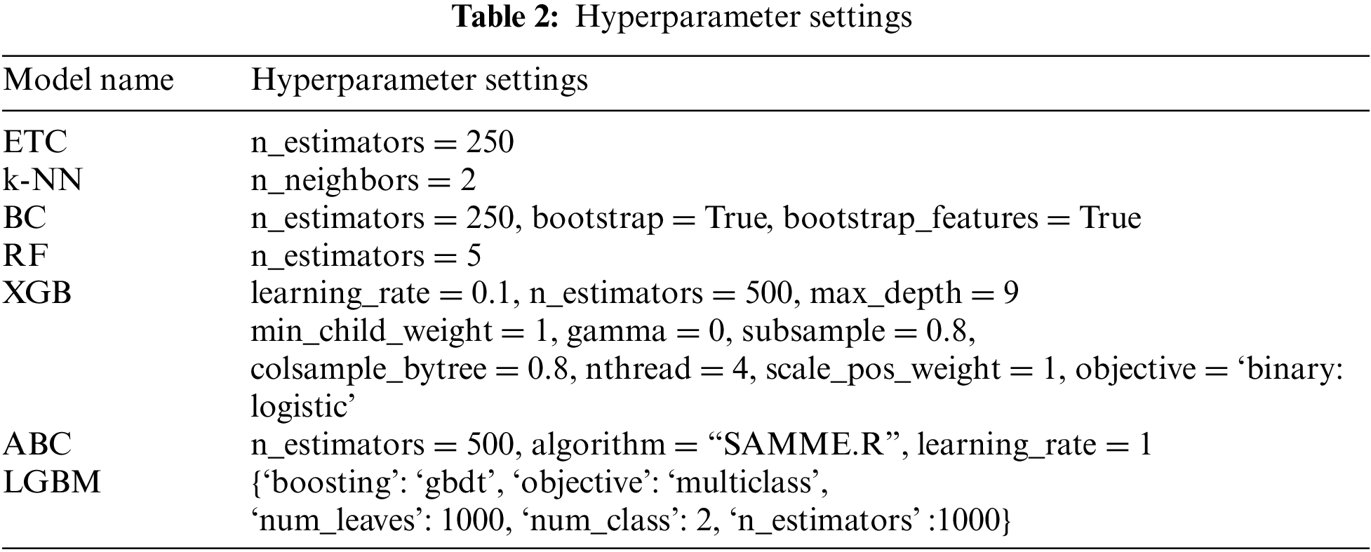
4.1 Hyperparameters of Selected ML-Based Algorithms

Hyperparameter tuning is a vital element in developing ML-based models. It involves systematically exploring alternative hyperparameter combinations to enhance the model’s performance. The major ML-based models settings fine-tuned during the intensive experimentation are summarised in Table 2 as follows:

4.2 Results of Selected ML-Based Algorithms

We report the performance outcomes of applying the various dimensionality reduction methods (PCA, FA, tSVD and IFDRT) that are discussed in Section 3.3 to the Machine Learning algorithm’s learning process on the BODMAS dataset. As previously indicated, we concentrate on lowering the model complexity by employing various feature reduction strategies to achieve a low-cost framework that is prepared to operate on adaptable devices. In conjunction with the dimensionality reduction approaches investigated, the different learning algorithms (ETC, k-NN, BC, RF, XGB, ABC and LGBM) will be evaluated for their efficacy and efficiency in categorising the BODMAS dataset samples in real-time scenarios. To ensure a fair comparison between (PCA, FA, tSVD, and IFDRT), the number of components is set to equal 2, 5 and 10. That’s why we seek the minimum number of features yielding the maximum score.

4.2.1 PCA

Here, we present the findings from the several experiments conducted on the featured machine algorithms, using the PCA dimensionality reduction technique that was previously discussed and demonstrated in this work. The achieved results are given in Table 3.

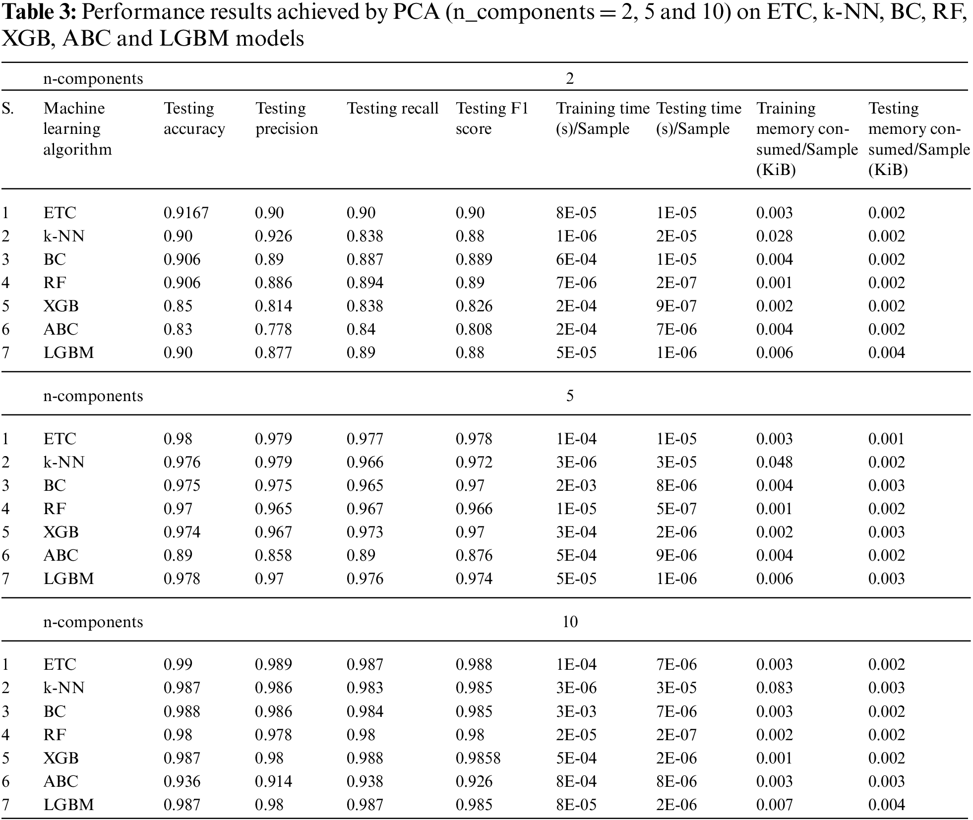
The presented results in Table 3 illustrate the performance of various Machine Learning algorithms (ETC, k-NN, BC, RF, XGB, ABC, and LGBM) on the BODMAS dataset using Principal Component Analysis (PCA) for dimensionality reduction with different numbers of components (2, 5, and 10). The results show the metrics of testing accuracy, precision, recall, F1 score, training and testing time per sample, and memory consumption per sample during the training and testing phases. Notably, as the number of components increased from 2 to 10, the models’ performance metrics generally improved. For example, with ten components, the Extra Trees Classifier (ETC) achieved a testing accuracy of 0.99, and similar high performance was observed for other algorithms like k-NN, BC, and RF, which all achieved near-perfect scores. The LGBM model also performed exceptionally well, achieving an F1 score of 0.985 with ten components. These results indicate that the results from the archives, when using only two components, are insufficient for use in actual production environments. So, in the following parts, we will look into the other dimensionality reduction techniques in more details.

4.2.2 FA

Here, we present the findings from the several experiments conducted on the featured machine algorithms, using the FA dimensionality reduction technique was previously discussed and demonstrated in this work. The achieved results are given in Table 4. The number of components for which the experiments were carried out was 2, 5 and 10. The assessments were averaged after being run twenty times.

The results in Table 4 showcase the performance of various Machine Learning algorithms on the BODMAS dataset using Factor Analysis (FA) for dimensionality reduction with the same different numbers of components (2, 5, and 10). As observed, the models generally improved their performance metrics with an increasing number of components. For instance, with ten components, the Extra Trees Classifier (ETC) achieved a testing accuracy of 0.988 and an F1 score of 0.986, demonstrating robust performance. Similarly, k-NN, BC, and RF also exhibited high accuracy and F1 scores near 0.98. LGBM consistently performed well across different component numbers, achieving an F1 score of 0.984 with ten components. These findings suggest that the results from the archives, when using only two or five components are insufficient for use in actual production environments. So, in the following parts, we will look into the other dimensionality reduction techniques in more details.

4.2.3 tSVD

Here, we present the findings from the experiments conducted on the featured machine algorithms using the famous and powerful tSVD dimensionality reduction technique that was previously discussed and demonstrated in this work. The assessments were averaged after being run twenty times, as indicated in Table 5.

The results in Table 5 underscore the effectiveness of tSVD in enhancing the performance metrics of the models when compared to the PCA and FA scenarios. Notably, in the tSVD example, the LGBM model exhibited the highest accuracy, reaching 89% with an F1 score of 0.88. However, it’s worth noting that the LGBM model’s performance plateaued with 2, 5 and 10 components, suggesting that further dimensionality reduction with tSVD is the worst performing compared with PCA and FA; thus it cannot be used for real implementation on the intended dataset.

4.2.4 IFDRT

In the last set of experiments, three values of components—2, 5, and 10—were examined utilising the innovative IFDRT dimensionality reduction technique. In particular, the three factors that were assessed: classification accuracy, memory consumption and computation time for feature reduction, model training and prediction processes. The assessments were averaged after being run twenty times, as indicated in Table 6.

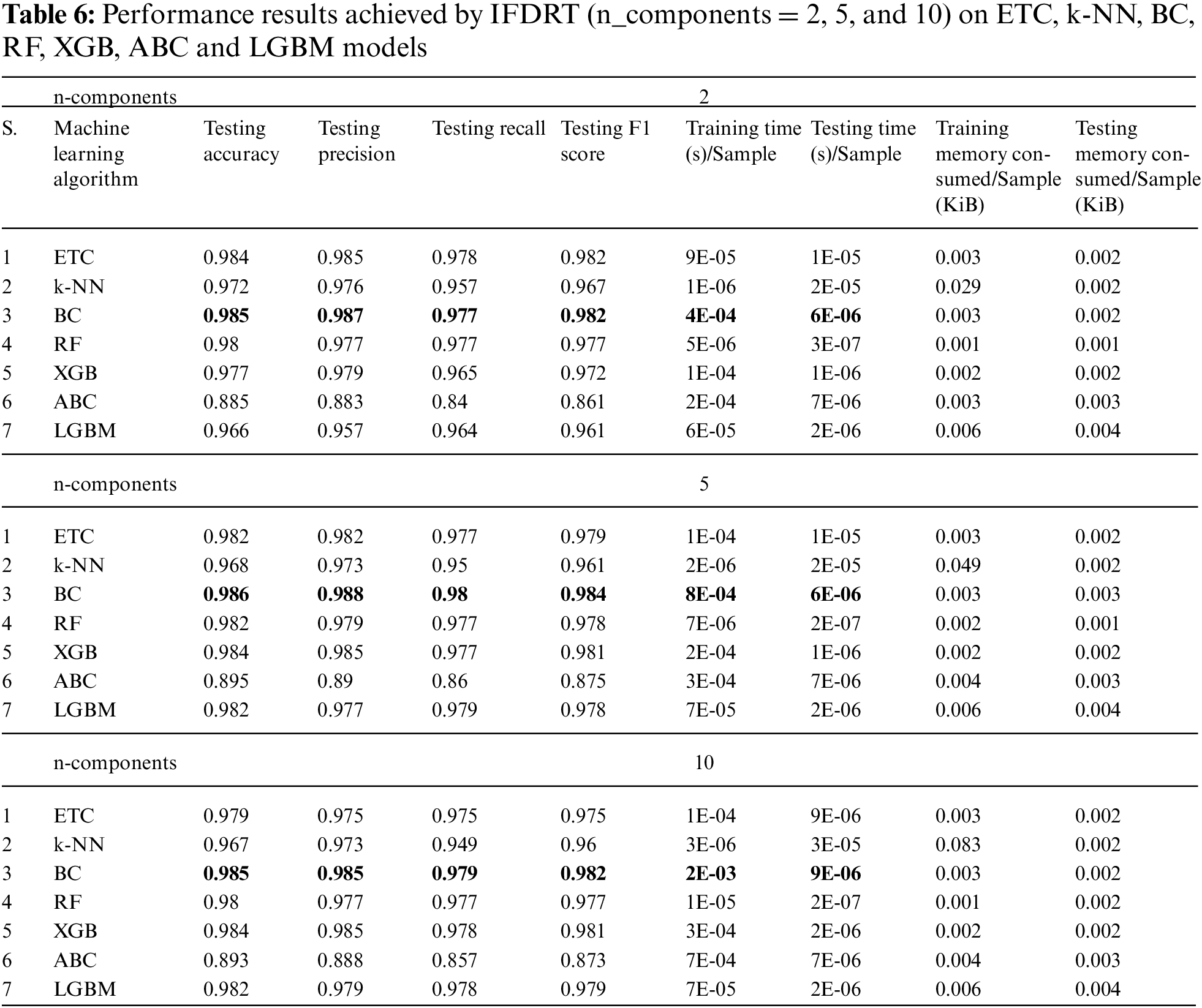
Table 6 highlights the performance of various ML-models with the IFDRT dimensionality reduction technique. Specifically, models like, ETC, BC and XGB exhibited noteworthy results across different numbers of components. For instance, with two components, etc., achieved an accuracy of 98.4% and an F1 score of 98.2%, indicating robust performance even with reduced feature dimensionality. BC maintained high accuracy across all component numbers, achieving 98.5% accuracy with two components and maintaining 98.5% with 5 and 10 components, showcasing stability in its performance. XGB also demonstrated consistent accuracy and F1 scores across varying component numbers, with an accuracy of 97.7% and an F1 score of 97.2% with two components. These results suggest that the IFDRT technique effectively preserves the discriminative information necessary for accurate classification, enabling these models to perform well even with reduced feature sets.

When it came to Training and Prediction Times, RF was superior. We observed an increase in Training and Prediction Time concerning the LGBM in the last group. Undoubtedly, the XGB has successfully balanced Accuracy and Training and Prediction Times—two crucial requirements in the real-world business settings of use cases. As a result, we conclude that the BC or XGB model, when combined with IFDRT, can be considered for actual business scenarios in Malware Classification systems with the best detection accuracy and real-time processing capabilities at the lowest possible requirements.

Another experiment is performed to assess the performance of IFDRT on the best-performing ML-model which is BC, against the other anticipated dimensionality reduction techniques. Fig. 7 shows that IFDRT outperformed other well-known feature dimensionality reduction approaches when employing two and five components, which is precisely what we expected from IFDRT. Another point to note is that IFDRT clearly beats the other techniques when n_component is set to two. An incease of 8% had been recorded in favor of IFDRT. This is an significant discovery that we should emphasize in this experiment. We conclude that IFDRT beats all other approaches for both two and five components. Another finding found that tSVD was the least effective approach on the BODMAS dataset. The greatest testing accuracy attained was 0.905, independent of the n_component value.

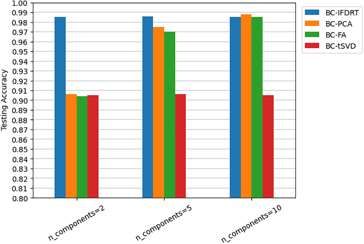
Figure 7: Testing accuracy of BC ML-model over IFDRT, PCA, FA, and tSVD for multiple n_components (2, 5 and 10)

Fig. 8 depicts the confusion matrix of all models for testing phases when using only two components. We can notice the superiority of both ETC, and BC with the lowest numbers in the black squares. This proves the balanced performance of those two models among the other models in terms of false positives and negatives.

Figure 8: Confusion matrix for ML-Models (n_components = 2). (a) ETC, Confusion matrix; (b) k-NN Confusion matrix; (c) BC Confusion matrix; (d) RF Confusion matrix; (e) XGB Confusion matrix; (f) ABC Confusion matrix; (g) LGBM Confusion matrix

4.3 IFDRT n_Components Effect Investigation

As the number of components incorporated into the training, optimising, and prediction phases of ML-based models affects the computational complexity, we tested the complexity and efficiency of the proposed IFDRT method in terms of Memory and CPU time consumption. Therefore, we set the n_components to 2, 5 and 10 values. In Fig. 9, we notice an increase in memory consumption with the increase of n_components with a maximum of 0.040 KiB per sample when n_components is equal to 10. However, the maximum consumed time of computation is achieved when n_components is equal to 2, 5 and 10 with no more than a fraction of 2E-03 second per sample, which is both subtle and feasible to apply in real-world applications.

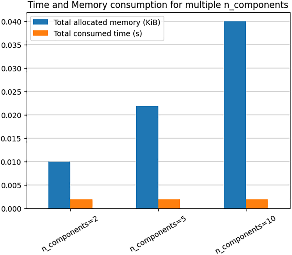
Figure 9: IFDRT CPU time and memory consumption

4.4 Comparison Analysis

To illustrate the usefulness of the proposed ML-models for malware detection, we compared our results to those from earlier research that utilised the BODMAS dataset [25,26]. Table 7 compares many performance metrics, including accuracy, precision, recall, and F1 score. The comparison is done objectively, considering previous experiments may have used different parameters, such as validation procedures and training/testing sample sizes. This study demonstrates that the best ML-based models devised for the BODMAS dataset exceed previous studies, yielding superior results.

Table 7 shows that our proposed IFDRT on BC outperforms all previous algorithms based on CNN and Transformer. It’s worth noting that we only used five reduced features instead of all 2381 feature vectors. It is a substantial improvement, requiring significantly less computing to predict and analyse malware during real-time applications while achieving greater accuracy. Considering F1 score metric, we can see a noticeable improvement over [25,26]. In summary, the IFDRT method devised in this work outperforms or matches the CNN and Transformer algorithms in terms of precision and F1 score while maintaining competitive accuracy and recall. This highlights the effectiveness of IFDRT in achieving balanced performance across multiple metrics. Keep in mind that CNN and Tranformers are both time-consuming algorithms based on Deep Learning, which is constructed using time-consuming procedures.

To the best of our knowledge, among dimensionality reduction approaches, our IFDRT is being employed for the first time to transform numeric features with the highest accuracy with a minimum number of features. Our findings are excellent and have the potential to provide a comprehensive system that can be used in a variety of contexts to identify and respond to sophisticated malware at the individual, corporate, and governmental levels while minimising computational costs through the use of high-performing classifiers during training.

5  Conclusions

In conclusion, this research study has presented a unique lightweight approach to malware classification that combines ML-models with a novel interpolation-based feature dimensionality reduction strategy. Through rigorous experimentation and evaluation, our proposed technique has proven promising results in accurately identifying malware samples while effectively lowering the dimensionality of the feature space and detection time.

Our research tackles the fundamental difficulty of dealing with high-dimensional data in malware classification tasks, where typical Machine Learning methods may suffer due to dimensionality’s curse. Using interpolation-based dimensionality reduction, we substantially decrease feature space while retaining the discriminative information required for effective classification.

The experimental results on BODMAS benchmark malware datasets show that our proposed method outperforms existing approaches regarding classification accuracy, precision, recall, and F1 score. The achieved accuracy of 0.986 and F1 score of 0.984 is attributable to the superiority of the proposed IFDRT, which employs just five components out of 2381 features from the BODMAS dataset. Furthermore, our method’s computational efficiency makes it appropriate for real-world applications requiring speedy malware identification and classification while operating on devices with limited resources.

Overall, this study advances the area of malware classification by presenting a unique technique that blends ML-models and interpolation-based dimensionality reduction. The findings described in this research have important significance for cybersecurity practitioners since they provide a potent weapon for battling the ever-changing world of malware threats.

6  Future Work

While the suggested IFDRT approach has shown promising results in real-time malware detection, there are numerous areas where future studies might improve its performance and applicability. Expanding the application using Deep Learning techniques might be considered to improve model performance. IFDRT current implementation focuses on identifying known malware patterns. Future studies might look into how IFDRT can be used to detect anomalies in real time, allowing the identification of unknown or zero-day malware variants. With the expansion of IoT devices, there is an increasing demand for effective malware detection systems that can run on resource-constrained devices. Future research might look at the viability of putting IFDRT and Deep learning on real operations on edge computing platforms and IoT devices, providing real-time malware detection in these contexts.

Acknowledgement: The authors would like to acknowledge the support of Princess Nourah bint Abdulrahman University Researchers Supporting Project number (PNURSP2024R435), Princess Nourah bint Abdulrahman University, Riyadh, Saudi Arabia and Al-Zaytoonah University of Jordan for their continuous support of this work.

Funding Statement: This reseach is funded by Princess Nourah bint Abdulrahman University Researchers Supporting Project number (PNURSP2024R435), Princess Nourah bint Abdulrahman University, Riyadh, Saudi Arabia.

Author Contributions: All Authors contributed equally. The authors confirm contribution to the paper as follows: study conception and design: Mahmoud E. Farfoura, Ahmad Alkhatib, Deema Mohammed Alsekait; data collection: Mohammad Alshinwan, Sahar A. El-Rahman; analysis and interpretation of results: Deema Mohammed Alsekait, Diaa Salama AbdElminaam; draft manuscript preparation: Didi Rosiyadi, Diaa Salama AbdElminaam; supervision, methodology, conceptualization, formal analysis, writing—review & editing: Mahmoud E. Farfoura, Ahmad Alkhatib. All authors reviewed the results and approved the final version of the manuscript.

Availability of Data and Materials: The data is available with the corresponding author and can be shared on request.

Ethics Approval: Not applicable.

Conflicts of Interest: The authors declare that they have no conflicts of interest to report regarding the present study.

References

1. S. Fayyad, A. Ahmed, and M. Hossain, “A methodology for dynamic security risks assessment in interconnected IT systems,” J. Commun. Softw. Syst., vol. 20, no. 1, pp. 13–22, 2024. doi: 10.24138/jcomss-2023-0128. [Google Scholar] [CrossRef]

2. Z. Mohammad, A. A. Alkhatib, M. Lafi, A. Abusukhon, D. Albashish and J. Atwan, “Cryptanalysis of a tightly-secure authenticated key exchange without NAXOS approach based on decision linear problem,” in 2021 Int. Conf. Inform. Technol. (ICIT), Amman, Jordan, 2021, pp. 218–223. doi: 10.1109/ICIT52682.2021.9491743. [Google Scholar] [CrossRef]

3. M. Farfoura, S. Horng, J. Lai, R. Run, R. Chen and M. Khan, “A blind reversible method for watermarking relational databases based on a time-stamping protocol,” Expert Syst. Appl., vol. 39, no. 3, pp. 3185–3196, 2012. doi: 10.1016/j.eswa.2011.09.005. [Google Scholar] [CrossRef]

4. D. J. Smith and K. G. Simpson, The Safety Critical Systems Handbook: A Straightforward Guide to Functional Safety. IEC 61511 (2015 Edition) and Related Guidance. Oxford, UK: Butterworth-Heinemann. 2020. Accessed: Aug. 7, 2024. [Online]. Available: https://books.google.com.eg/books?id=IXLKDwAAQBAJ&#x0026;lpg=PP1&#x0026;ots=GaujsHQVHW&#x0026;dq=D.%20Smith%2C%20K.%20Simpson%2C%20%E2%80%9CThe%20Safety%20Critical%20Systems%20Handbook%E2%80%9D%2C%20Elsevier%2C%20Amsterdam%2C%20The%20Netherlands%2C%202010.&#x0026;lr&#x0026;pg=PR3#v=onepage&#x0026;q&#x0026;f=false [Google Scholar]

5. A. Damodaran, F. Troia, C. Visaggio, T. Austin, and M. Stamp, “Comparison of static, dynamic, and hybrid analysis for malware detection,” J. Comput. Virol. Hacking Tech., vol. 13, no. 1, pp. 1–12, 2017. doi: 10.1007/s11416-015-0261-z. [Google Scholar] [CrossRef]

6. M. Siddiqui, M. Wang, and J. Lee, “A survey of data mining techniques for malware detection using file features,” in Proc. 46th Annu. Southeast Reg. Conf. (ACM-SE 46), New York, NY, USA, Association for Computing Machinery, 2008, pp. 509–510. [Google Scholar]

7. J. Rabek, R. Khazan, S. Lewandowski, and R. Cunningham, “Detection of injected, dynamically generated, and obfuscated malicious code,” in Proc. 2003 ACM Workshop Rapid Malcode, 2003, pp. 76–82. [Google Scholar]

8. K. Wang and S. J. Stolfo, “Anomalous payload-based network intrusion detection,” in Recent Advances in Intrusion Detection, Berlin, Heidelberg: Springer, Sep. 2004, vol. 3224, pp. 203–222. doi: 10.1007/s11416-015-0261-z. [Google Scholar] [CrossRef]

9. C. Taylor and J. Alves-Foss, “NATE–network analysis of anomalous traffic events, a low-cost approach,” in New Security Paradigms Workshop, New York, NY, USA: Association for Computing Machinery (ACM), 2001. [Google Scholar]

10. M. Boldt and B. Carlsson, “Analysing privacy-invasive software using computer forensic methods,” Jan. 2006. Accessed: Aug. 28, 2024. [Online]. Available: https://www.researchgate.net/publication/249717066_Analysing_Privacy-Invasive_Software_Using_Computer_Forensic_Methods [Google Scholar]

11. R. Sekar, M. Bendre, D. Dhurjati, and P. Bollineni, “A fast automaton-based method for detecting anomalous program behaviors,” in Proc. 2001 IEEE Symp. Secur. Priv. S&P 2001, Oakland, CA, USA, 2001, pp. 144–155. [Google Scholar]

12. S. Hofmeyr, S. Forrest, and A. Somayaji, “Intrusion detection using sequences of system calls,” J. Comput. Secur., vol. 6, no. 3, pp. 151–180, 1998. doi: 10.3233/JCS-980109. [Google Scholar] [CrossRef]

13. W. Li, K. Wang, S. Stolfo, and B. Herzog, “Fileprints: Identifying file types by n-gram analysis,” in Proc. Sixth Annu. IEEE SMC Inform. Assur. Workshop, West Point, NY, USA, 2005, pp. 64–71. [Google Scholar]

14. S. Forrest, A. S. Perelson, L. Allen, and R. Cherukuri, “Self-nonself discrimination in a computer,” in Proc. 1994 IEEE Comput. Soc. Symp. Res. Secur. Priv., Oakland, CA, USA, 1994, pp. 202–212. [Google Scholar]

15. C. Ko, M. Ruschitzka, and K. Levitt, “Execution monitoring of security-critical programs in distributed systems: A specification-based approach,” in Proc. 1997 IEEE Symp. Secur. Priv. (Cat. No. 97CB36097), Oakland, CA, USA, 1997, pp. 175–187. [Google Scholar]

16. J. Xiong, “ACT: Attachment chain tracing scheme for email virus detection and control,” in Proc. ACM Workshop Rapid Malcode (WORM), 2004. [Google Scholar]

17. M. Debbabi, E. Giasson, B. Ktari, F. Michaud, and N. Tawbi, “Secure self-certified cots,” in Proc. 9th IEEE Int. Workshops Enabling Technol.: Infrastruct. Collab. Enterp., 2000, pp. 183–188. [Google Scholar]

18. E. Filiol, “Malware pattern scanning schemes secure against black-box analysis,” J. Comput. Virol, vol. 2, pp. 35–50, 2006. doi: 10.1007/s11416-006-0009-x. [Google Scholar] [CrossRef]

19. I. Baptista, S. Shiaeles, and N. Kolokotronis, “A novel malware detection system based on machine learning and binary visualization,” in 2019 IEEE Int. Conf. Commun. Workshops (ICC Workshops), Shanghai, China, 2019, pp. 1–6. [Google Scholar]

20. D. Vu, T. Nguyen, T. V. Nguyen, T. N. Nguyen, F. Massacci and P. H. Phung, “HIT4Mal: Hybrid image transformation for malware classification,” Trans. Emerg. Telecommun. Technol., vol. 31, no. 11, pp. 1–15, 2019. [Google Scholar]

21. W. K. Wong, F. H. Juwono, and C. Apriono, “Vision-based malware detection: A transfer learning approach using optimal ECOC-SVM configuration,” IEEE Access, vol. 9, pp. 159262–159270, 2021. [Google Scholar]

22. M. Xiao, C. Guo, G. Shen, Y. Cui, and C. Jiang, “Image-based malware classification using section distribution information,” Comput. Secur., vol. 110, 2021, Art. no. 102420. doi: 10.1016/j.cose.2021.102420. [Google Scholar] [CrossRef]

23. Z. Xu, K. Ren, S. Qin, and F. Craciun, “CDGDroid: Android malware detection based on deep learning using CFG and DFG,” Formal Methods Softw. Eng., vol. 11232, pp. 177–193, 2018. doi: 10.1007/978-3-030-02450-5. [Google Scholar] [CrossRef]

24. A. R. Nasser, A. M. Hasan, and A. J. Humaidi, “DL-AMDet: Deep learning-based malware detector for android,” Intell. Syst. Appl., vol. 21, 2024, Art. no. 200318. doi: 10.1016/j.iswa.2023.200318. [Google Scholar] [CrossRef]

25. J. Hao, S. Luo, and L. Pan, “EII-MBS: Malware family classification via enhanced instruction-level behavior semantic learning,” Comput. Secur., vol. 112, no. C, 2022, Art. no. 102905. doi: 10.1016/j.cose.2022.102905. [Google Scholar] [CrossRef]

26. Q. Lu, H. Zhang, H. Kinawi, and D. Niu, “Self-attentive models for real-time malware classification,” IEEE Access, vol. 10, pp. 95970–95985, 2022. [Google Scholar]

27. L. Onwuzurike, E. Mariconti, P. Andriotis, E. D. Cristofaro, G. Ross and G. Stringhini, “MaNaDroid: Detecting android malware by building markov chains of behavioral models (extended version),” ACM Trans. Priv. Secur., vol. 22, no. 2, pp. 1–34, 2019. doi: 10.1145/3313391. [Google Scholar] [CrossRef]

28. L. Yang, A. Ciptadi, I. Laziuk, A. Ahmadzadeh, and G. Wang, “BODMAS: An open dataset for learning based temporal analysis of PE malware,” in 2021 IEEE Secur. Priv. Workshops (SPW), San Francisco, CA, USA, 2021, pp. 78–84. [Google Scholar]

29. J. Smith and M. Johnson, “Using principal component analysis to reduce dimensionality in dataset,” J. Stat., vol. 23, no. 4, pp. 67–78, 2018. [Google Scholar]

30. J. Smith and M. Johnson, “Principal factor analysis: A statistical approach for reducing dimensionality,” J. Multivar. Anal., vol. 36, no. 2, pp. 45–57, 2019. [Google Scholar]

31. P. C. Hansen, “Truncated singular value decomposition and applications,” IEEE Trans. Signal Process., vol. 35, no. 3, pp. 554–565, 1987. [Google Scholar]

32. A. Mughaid, S. AlZu’bi, and A. Hnaif, “An intelligent cyber security phishing detection system using deep learning techniques,” Clust. Comput., vol. 25, pp. 3819–3828, 2022. doi: 10.1007/s10586-022-03604-4. [Google Scholar] [PubMed] [CrossRef]

33. H. M. Al-Mimi, N. A. Hamad, M. M. Abualhaj, S. N. Al-Khatib, and M. O. Hiari, “Improved intrusion detection system to alleviate attacks on DNS service,” J. Comput. Sci., vol. 19, no. 12, pp. 1549–1560, 2023. doi: 10.3844/jcssp.2023.1549.1560. [Google Scholar] [CrossRef]

34. P. Domingos, “A few useful things to know about machine learning,” Commun. ACM, vol. 55, no. 10, pp. 78–87, 2012. doi: 10.1145/2347736.2347755. [Google Scholar] [CrossRef]

35. K. He, X. Zhang, S. Ren, and J. Sun, “Deep residual learning for image recognition,” in 2016 IEEE Conf. Comput. Vis. Pattern Recognit. (CVPR), Las Vegas, NV, USA, 2016, pp. 770–778. [Google Scholar]

36. P. Geurts, D. Ernst, and L. Wehenkel, “Extremely randomised trees,” Mach. Learn., vol. 63, no. 1, pp. 3–42, 2006. doi: 10.1007/s10994-006-6226-1. [Google Scholar] [CrossRef]

37. E. Fix and J. L. Hodges, Discriminatory Analysis: Nonparametric Discrimination: Consistency Properties. American Psychological Association, 1951. doi: 10.1037/e471672008-001. [Google Scholar] [CrossRef]

38. L. Breiman, “Bagging predictors,” Mach. Learn., vol. 24, no. 2, pp. 123–140, 1996. doi: 10.1007/BF00058655. [Google Scholar] [CrossRef]

39. T. K. Ho, “Random decision forests,” in Proc. 3rd Int. Conf. Doc. Anal. Recognit., Montreal, QC, Canada, 1995, vol. 1, pp. 278–282. [Google Scholar]

40. T. Q. Chen and C. Guestrin, “XGBoost: A scalable tree boosting system,” in Proc. 22nd ACM SIGKDD Int. Conf. Knowl. Discov. Data Min., 2016, pp. 785–794. [Google Scholar]

41. F. Yoav and R. E. Schapire, “A decision-theoretic generalization of on-line learning and an application to boosting,” J. Comput. Syst. Sci., vol. 55, no. 1, pp. 119–139, 1997. doi: 10.1006/jcss.1997.1504. [Google Scholar] [CrossRef]

42. G. Ke et al., “LightGBM: A highly efficient gradient boosting decision tree,” Adv. Neural Inf. Process Syst., vol. 30, pp. 3146–3154, 2017. [Google Scholar]