Knowledge-Driven Possibilistic Clustering with Automatic Cluster Elimination

1  Introduction

Clustering is an unsupervised machine learning methodology that offers a suite of algorithms to discover a structure in the given unlabeled dataset. Clustering techniques have been widely applied in various fields such as industrial chains [1], collective intelligence [2], and image processing [3,4]. Depending on whether additional knowledge hints are incorporated into the clustering process, clustering algorithms can be classified into data-driven and knowledge-driven. The classical objective function-based K-means [5] and FCM algorithms [6,7], as well as some improved algorithms [8–11] are data-driven clustering algorithms. Data-driven clustering uncovers the potential structure by only considering the relationships present in the unlabeled data, thus ignoring the impact of domain knowledge on clustering. This clustering process lacks a clear search direction, resulting in a slower completion of the clustering task [12,13]. As opposed to data-driven clustering, knowledge-oriented clustering increases the consideration of compatibility with knowledge hints so that the overall optimization process focuses on a specific search direction, thus improving the effectiveness [12–15].

Knowledge-driven clustering simulates the process of differentiating items in reality, that is, purposefully and quickly finding specific objects when provided with extra knowledge hints. For example, in the fuzzy clustering with viewpoints (V-FCM) algorithm proposed by Pedrcyz et al., the knowledge hints (called viewpoints) are extreme data (minimum, maximum, medium, etc.) [12]. Those viewpoints directly replace some of the prototypes during the optimization process as a way to achieve the navigation of a personalized search for the structure. Based on this knowledge-driven clustering framework, Tang et al. proposed possibilistic fuzzy clustering with a high-density viewpoint (DVPFCM) algorithm [13]. The DVPFCM algorithm replaces the personality viewpoints in the V-FCM algorithm with a high-density point to guide the algorithm to find centers closer to the actual data structure. Compared with V-FCM, the DVPFCM algorithm is more robust. To better deal with datasets with irregular structures, Tang et al. proposed the Knowledge-induced Multiple Kernel Fuzzy Clustering (KMKFC) in which the kernel distance is adopted [14]. However, V-FCM, DVPFCM, and KMKFC all output domain knowledge as part of the prototype and change the partition matrix U directly, which means that some clustering results are determined before the algorithm is executed. The flexibility of the algorithm is greatly limited, and the domain knowledge has too much influence.

In addition to these V-FCM-based algorithms, transfer clustering is another type of knowledge-based clustering. The self-taught clustering proposed in [16] which is a transfer clustering strategy based on the strength of mutual information. Jiang et al. [17] introduced the transfer learning idea into spectral clustering and then presented the transfer spectral clustering algorithm. Reference [18] introduced the concept of transfer learning to prototype-based fuzzy clustering and provided two clustering algorithms. The core idea of these algorithms is to extract knowledge from an auxiliary dataset and then improve the learning ability of the target dataset. However, there are not always auxiliary data to help cluster the target data in reality. Moreover, the number of clusters in knowledge-driven clustering based on the idea of V-FCM and transfer clustering is given in advance. However, in reality, the value of this parameter is difficult to obtain directly.

The research progress in knowledge-driven clustering shows that most studies focus on knowledge utilization related to the clustering center location to locate the final clustering centers more accurately or with more personality viewpoints. However, another factor that affects the performance of clustering algorithms, the number of clusters, is ignored. Existing knowledge-driven clustering algorithms are predicated on the premise that this domain knowledge is given in advance, but in reality, the number of clusters is hard to determine, and it has a significant impact on the effectiveness of clustering [19,20]. The number of clusters directly influences the granularity of the grouping and the interpretability of the results. If the number of clusters is too high, the algorithm might overfit the data, resulting in too many small, fragmented clusters that fail to reveal meaningful patterns. Conversely, if the number of clusters is too low, the algorithm might underfit the data, merging distinct groups and obscuring important differences.

A simple and direct way to determine the number of clusters is to use a cluster validity index (CVI) to measure the clustering performance under different numbers of clusters and then select the number of groups corresponding to the best metric value as the optimal number of clusters. This is also a common approach in the current clustering field to detect the correct number of clusters [20–22]. However, this method has the issues of costly computation and excessive testing of clustering numbers (usually ranging from 2 to the square root of the sample numbers, with an increment of 1), as well as the problem of obtaining different optimal cluster numbers with different CVIs [23]. Rodriguez and Laio proposed a density peak clustering (DPC) algorithm which identifies cluster centers based on two key criteria: high local density and a large distance from other points with higher densities [24]. It does not require a predefine cluster number but allows manual selection based on the decision graph. However, its time complexity is high, at 𝒪(n2) where N is the number of samples. Consequently, some methods have been proposed to reduce this time cost, such as fast clustering with local density peaks-based minimum spanning tree (Fast LDP-MST) and the Granular ball-based density peak (GB-DP) algorithm [25,26]. Fast LDP-MST designs a more effective method based on minimum spanning tree to reduce the time complexity of DPC to 𝒪(Nlog⁡(N)). The GB-DP algorithm uses granular computing techniques to reduce the original dataset into smaller granules, and then applies the DPC algorithm to cluster these granulated datasets, significantly reducing the algorithm’s time complexity. Although algorithms based on DPC do not require the number of clusters to be predefined and have reduced time complexity, the DPC algorithm is sensitive to the parameter density radius r. Additionally, DPC is a hard clustering algorithm, exhibiting binary characteristics. This binary nature can make it difficult to handle fuzzy boundaries between data points in some cases.

Facing these challenges, our work in this paper attempts to adaptively determine the optimal number of clusters during the clustering process through knowledge guidance. The knowledge extraction algorithm, DKPE, which is proposed first, obtains knowledge tidbits, i.e., high-density points, that help determine the positions of cluster centers. The initial number of clusters is fixed at twice the number of high-density points, which is obviously greater than the actual number of clusters. Finally, combined with the merging clusters schema, the HP-PCM algorithm eliminates redundant cluster centers based on the influence of high-density points. In this way, the proper number of clusters is determined.

By integrating automatic cluster elimination, our approach not only reduces computational overhead but also enhances the consistency and reliability of clustering results. This ensures that high-quality clustering solutions are achieved across various datasets and application scenarios, thereby improving the overall performance and applicability of knowledge-driven clustering algorithms. Moreover, in [12–14], knowledge tidbits directly replaced part of the family of prototypes, resulting in ineffective iterative updates of some cluster centers, as these centers are predetermined before clustering. In this way, the flexibility of the algorithm is severely limited. Therefore, in the proposed clustering algorithm, HP-PCM, adaptive influence weights for knowledge tidbits and a term to measure the matching degree between knowledge and cluster centers in the objective function are added. Our goal is to change the role of knowledge from a decision-maker to a guide, thus improving clustering performance while adaptively updating the cluster results (centers and membership degrees).

The contributions of our proposed HP-PCM algorithm can be summarized as follows:

•   We propose a new knowledge hints extraction method, DKPE, to provide more useful assistance for knowledge-driven clustering. The DKPE method can extract high-density and scattered data as knowledge hints, which are utilized in the HP-PCM algorithm as guides. Its operation is not complicated and does not require additional datasets.

•   The number of knowledge points is used as the basis for setting the initial number of clusters Cini to ensure that Cini is greater than the true value and to improve the efficiency of the algorithm in adaptively determining the final number of clusters.

•   We establish an improved objective function by balancing the relationship between clustering centers and knowledge hints (high-density points) and incorporating the merging clusters schema. This allows the HP-PCM algorithm to obtain more appropriate results and select parameters with a logical explanation.

The rest of this paper is organized as follows. In Section 2, we review the PCM-type and V-FCM-based algorithms. The motivation of this study is elaborated in Section 3. In Section 4, we present our proposed algorithms and their frameworks. The experimental results on synthetic datasets and the UCI datasets are described in Section 5. Finally, Section 6 presents our conclusions.

2  Related Work

In this section, PCM-type algorithms and V-FCM-based algorithms are briefly reviewed, and their main features are discussed. Consider the dataset X={xj}j=1N composed of N samples. The goal of these algorithms is to divide the data into C subsets to form the cluster center set V={vi}i=1C. Each sample xj and cluster center vi belong to Rl where l is the space dimensionality. The distance measure adopted in the algorithms is the Euclidean norm, denoted by ∥⋅∥. The iteration number of the algorithm is t, and the maximum iteration number is tMax.

2.1 PCM-Type Algorithms

The PCM algorithm is an improved FCM algorithm. It addresses the FCM algorithm’s sensitivity to noise by removing the sum-to-one constraint on membership degrees. In PCM, the compatibility of a point with a given cluster depends solely on the distance of the point from the corresponding cluster center. This approach eliminates the need to consider the point’s relationship with other clusters, thereby reducing the impact of outliers and noise on the updates to cluster centers.

PCM does not impose the sum-to-one limit, but a serious problem of the consistency of cluster centers may arise [27,28]. Improper γ values may lead PCM to fail to identify a sparse cluster located very close to a denser cluster, or it may even lead to a cluster center consistency problem [10,28]. To alleviate the shortcomings of PCM, scholars have proposed some improvements. The methods in [29–32] overcome the PCM algorithm cluster center consistency problem to a certain extent. Nevertheless, they cannot eliminate redundant classes if the number of initial clusters exceeds the actual value. Therefore, based on the idea of merging clusters [33], the PCM-type algorithms proposed in [10–11,34,35] have the cluster elimination abilities during their execution. Especially for the adaptive possibilistic clustering (APCM) and sparse-aware adaptive possibilistic clustering (SAPCM) algorithms proposed in [10,11], their update method of γ only considers the data points most relevant to the current center to enhance the flexibility and clustering ability of the algorithm.

However, the initial number of clusters in the abovementioned algorithms is set manually and lacks a reasonable explanation. More importantly, this setting directly affects the clustering performance, particularly in determining the correct number of final clusters [10,11].

2.2 V-FCM-Based Algorithms

The V-FCM algorithm proposed by Pedrycz et al. introduced the concept of “viewpoints” based on the FCM algorithm [12]. A viewpoint is the domain knowledge provided by a user, and it involves navigation for a personalized search of the structure. Viewpoints can be typical situations in data, such as the average, maximum, and minimum. Therefore, the V-FCM algorithm makes the clustering process more accessible with the help of the viewpoints, and the clustering results are more interpretable.

The viewpoints are defined by the two matrixes, denoted as B and F:

bik={1,if the kth feature of the ith propotype is from the viewpoint0,otherwisefik={y,bik=10,otherwise(1)

where y represents a specific value of the viewpoint. The V-FCM algorithm introduces knowledge hints, referred to as “viewpoints”, which result in a different updating equation for cluster centers compared to the FCM algorithm. As seen from (2), during the iteration process, the viewpoint fik remains fixed at the initial position of the prototype, and the parts not replaced by viewpoints need to be updated. This simplification of the clustering process allows for direct determination of clustering results, but it also reduces the flexibility of the V-FCM algorithm. Compared to the FCM algorithm, V-FCM can generate more reasonable and explainable clustering results, especially in extreme cases.

gik={∑j=1Nuijmxjk∑j=1Nuijm,bik=0fik,bik=1(2)

The DVPFCM and KMKF algorithms, which are improved versions of the V-FCM algorithms, improve the algorithm in terms of the knowledge type and distance formula, respectively, to obtain more accurate clustering results and increase its applicability. However, they all ignore the quality of knowledge and the unknown number of clusters, which can affect clustering performance.

3  Motivation

After describing the main characteristics of the PCM-type algorithms and the V-FCM-based algorithms, and based on the challenges mentioned in Section 1, the tasks of HP-PCM can be summarized as follows:

1.    to set the proper initial number of clusters (>true number);

2.    to adaptively obtain the optimal number of clusters;

3.    to balance the relationships of knowledge hints and cluster centers.

The first task is the basis for the second one. Most existing studies on the determination of the optimal cluster number set the initial value through human intervention, which may cause subjective bias. In this study, the first task is performed by proposing a knowledge extraction method, DKPE. This method provides P data points with a relatively high density and scattering distribution. P represents the approximate number of clusters of a dataset and can be used as a reference for setting Cini to be twice of P.

For the second task, we adopt the idea of merging clusters in APCM, but with an automatically determined suitable initial number of clusters. During each iteration, γis are updated by considering only the points that are most compatible with the corresponding vi. This allows the HP-PCM algorithm to discard invalid clusters and obtain the optimal clusters.

The final task is accomplished by adding a term to the objective function that balances the relationship between cluster centers and high-density points identified by the DKPE method. The influence of high-density points on the algorithm adapts during the iterative process, leading to cluster centers that optimize the objective function. The overall road map of HP-PCM is summarized in Fig. 1.

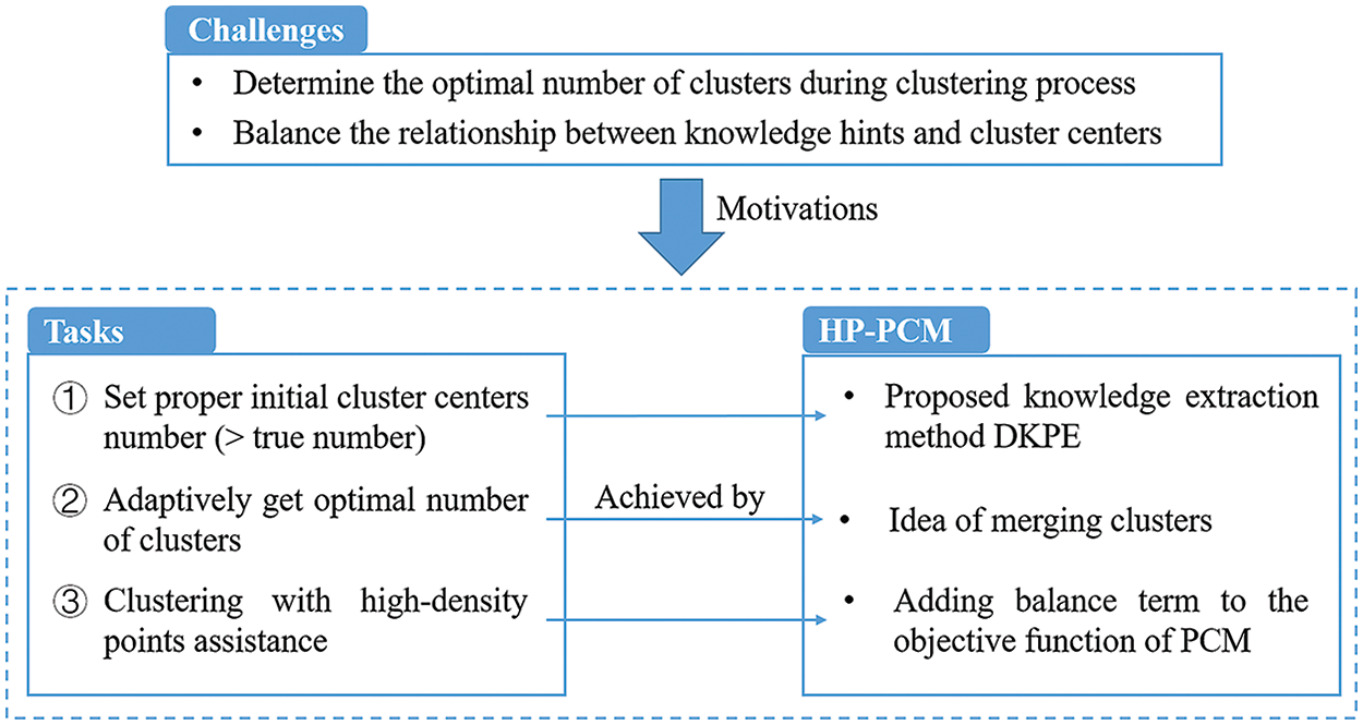
Figure 1: Road map of the proposed HP-PCM algorithm

4  Possibilistic C-Means Clustering with High-Density Points

This section establishes a knowledge extraction method, DKPE, and a novel clustering algorithm called the PCM clustering algorithm with high-density points (HP-PCM). The DKPE algorithm is designed to provide the HP-PCM algorithm with an appropriate number of initial clusters and high-density points (knowledge hints). Utilizing these knowledge hints, HP-PCM can automatically determine the optimal number of clusters during its clustering process.

4.1 Knowledge Extraction Method Based on Data Density

We propose the density knowledge points extraction (DKPE) method to select high-density points from the dataset as knowledge hints for the proposed HP-PCM clustering algorithm. The idea of DKPE is inspired by a clustering algorithm named clustering by a fast search and find of density peaks (DPC for short) [24].

The DPC algorithm involves calculating the local density and the relative distance between the data and data with higher local densities. This approach is straightforward to implement and ensures that the selected centers are well-dispersed. Similarly, the proposed DKPE method aims to extract high-density and scattered points as knowledge hints for the clustering algorithm. Although these two ideas are similar, the DPC method faces challenges in evaluating its density radius r. This parameter r determines the accuracy of DPC in estimating the density of data points, which in turn affects whether the algorithm can obtain true high-density points. In [24], the value of r is selected experimentally and adopts the first 1% to 2% of the ascending data distance. Furthermore, experiments in the next section show that the DPC centers are different from r in this interval for the same dataset.

The DPC algorithm is sensitive to the radius r but can get some high-density points. How can the performance of DPC be improved so that high-density points can be easily distinguished and extracted? To answer this question, we develop a novel density knowledge extraction method. We redefine the calculation of the local density of a sample xj as follows:

ρj=∑x∈KNN(xj)d(xj,xk),d(xj,xk)=∥xj−xk∥.(3)

where KNN(xj) represents the K-nearest neighbors of xj, K=⌊N⌋. The local density of a data point xj is the sum of its distances from the nearest K data points. The larger the value of ρj is, the farther the point xj deviates from other data points. In other words, the more scattered the data distribution around xj, the smaller its local density. ρj is negatively correlated with the density concept in [24]. Eq. (3) does not introduce other parameters but focuses on the value of K. It is assumed that the clustering problem is reasonable (i.e., N≫C) and a suitable upper bound of clusters number could be set to N in [36]. That is, the crowded areas of a dataset do not exceedN. For the limit idea, assuming N points of a dataset are evenly distributed in N crowded areas, there are N data points around each area. Additionally, those works using the concept of KNN also set K as N to make their algorithms have better performance [37–39]. That is, K=⌊N⌋ is also a commonly used rule. The local density of a data point in the center of a dense area is the highest, so the clustering center point close to the real data structure can be best screened by calculating the distance sum of the K other data points closest to the data point.

The search cost of KNN for each data point in the dataset is 𝒪(N), so the time complexity of DKPE is 𝒪(N2), which is huge. We introduce the KD-tree [40] into the DKPE algorithm to reduce the time complexity of DKPE to be 𝒪(Nlog⁡N).

If the clustering centers are determined by the local density values, it is possible to select some centers in the same dense area because their densities are estimated by the same K number of neighbors. In that case, their densities are also the same. There is a requirement to calculate another parameter δj(j∈{1,…,N}). Its formula is expressed as:

δj=min{d(xk,xj)|ρk<ρj,k∈{1,2,…,N}}.(4)

For the point with the smallest local density, δj=max{d(xk,xj)|j≠k,k∈{1,…,N}}(j∈{1,…,N}).

The data points selected by the DKPE algorithm have smaller ρ and larger δ values. So, they conform to the natural clustering centers characteristics. The DKPE algorithm calculates the local density of a data point based on the K nearest neighbors. Data points with a higher density can be generated semi-automatically, and are unaffected by the density radius r. The specific execution is shown in Algorithm 1.

4.2 Superiority of the Parameter K

Here, we illustrate the advantage of using the K-nearest neighbors to measure the data local density compared to measuring it with radius r in DPC. The used testing data is a 2-D synthetic dataset that is composed of three Gaussian clusters with centers v1=[0.0578,15.0039], v2=[−5.5063,12.5743], and v3=[4.7078,13.5072], and covariance matrices ∑1=[1.9745−0.0825−0.08250.5087], ∑2=[0.0656−0.0014−0.00140.0711], ∑3=[0.0540000.0503]. The three clusters are composed of 1000, 50, and 100 data points, respectively, making the sample size be N=1150. The data points belonging to the first, second, and third clusters are numbered 1 to 1000, 1001 to 1050, and 1051 to 1150, respectively. The data are shown in Fig. 2a.

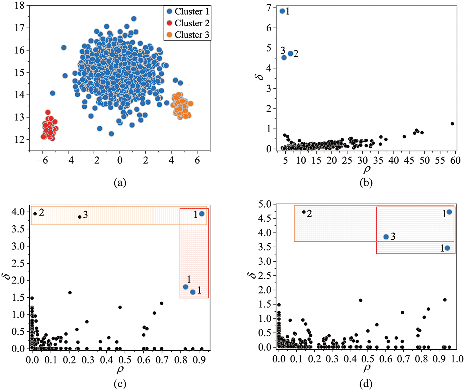
Figure 2: Synthetic dataset D1 and decision graphs of DPC and DKPE on D1. (a) Data distribution. Different colors represent different clusters. (b) DKPE decision graph with K=⌊N⌋=33. The numbers next to the dots are the cluster numbers to which the corresponding data point belongs. (c) Parameter r is the first 1% of the ascending data distance. (d) Parameter r is the first 2% of the ascending data distance

Comparing Fig. 2c,d, it can be found that setting r to the first 2% of the ascending distance provides the decision graph of DPC with a clearer gap between high-density points and non-high-density points than setting r to the first 1% of the distance. This means that the evaluation of local data density is sensitive to the value of r in DPC. In addition, the high-density points in the smaller cluster may be ignored or mistakenly identified as noise, leading to their exclusion—such as the black dot within the orange boxes in Fig. 2c,d. However, the data points chosen in the orange boxes of these two figures are scattered in different clusters, whereas the data points in the red boxes are concentrated within the same cluster.

In Fig. 2b, the high-density points are clearly located away from the non-high-density points, which makes the manual selection operation easy to perform and free of doubt. To show that the proposed DKPE algorithm is less sensitive to the value of K, we calculate the average distance d^ between the high-density points and the reference cluster centers obtained by DKPE and DPC for different values of K and r, respectively. K is varied in the interval [13,43] by an increase of 10. A smaller d^ indicates that the high-density points are closer to the dense areas. The formula of parameter d^ is:

d^=∑i=1Pd(gi,vi)P(5)

The calculation results are summarized in Table 1. The d^ value obtained by DKPE with different K values is approximately 0.1340, while this index exceeds 3.12 in DPC. This shows that DKPE provides a more reasonable measure of local data density based on K.

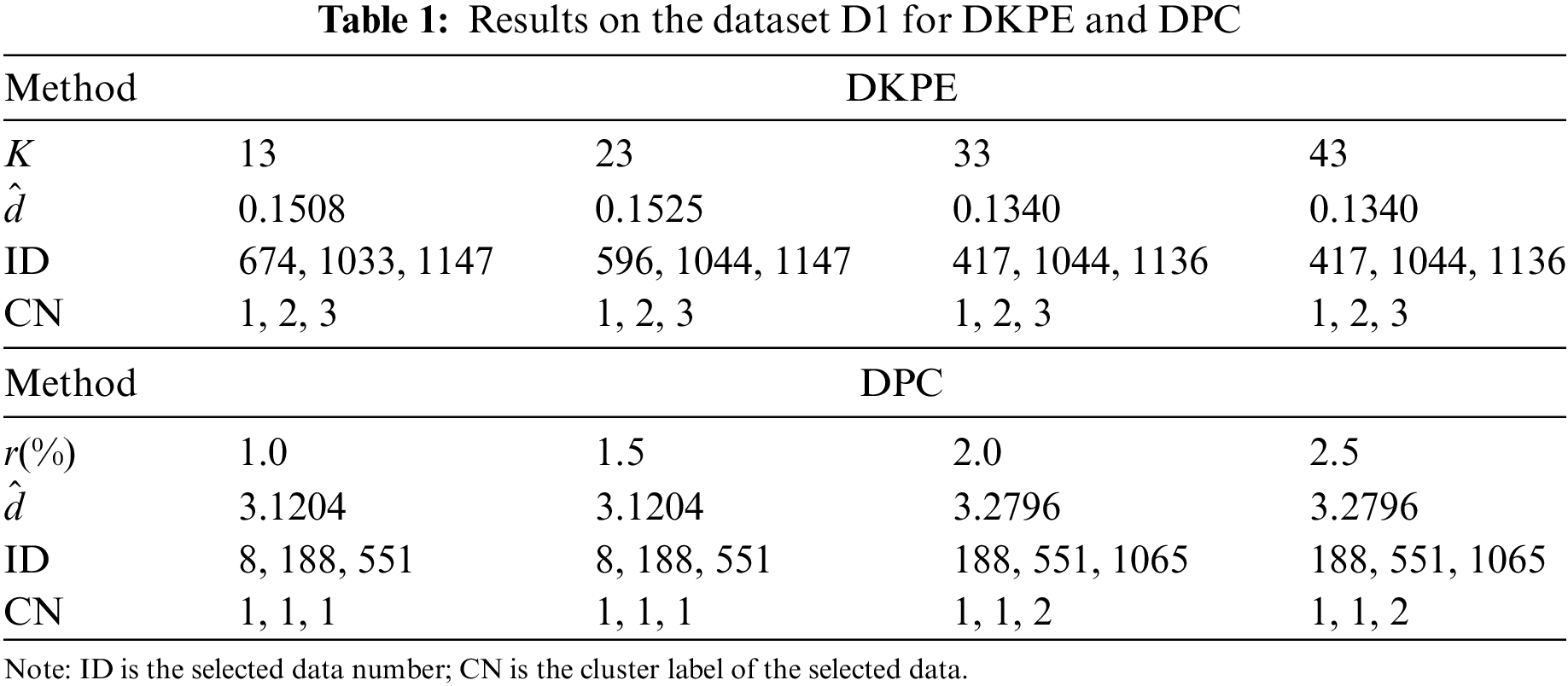
Changes in r can lead to variations in the number of data points surrounding the observed data point. In contrast, altering the value of K does not affect the average spacing between points. Within a certain range, the distribution of data points is relatively uniform. Therefore, DKPE can obtain high-density points more accurately and consistently.

4.3 Description of the Proposed HP-PCM Algorithm

Based on the proposed DKPE algorithm, we present the PCM clustering algorithm with high-density points (HP-PCM), and the goals of the algorithm are as follows:

1.    To balance the relationship between the high-density points identified by the DKPE method and the clustering centers, thereby preventing the high-density points from exerting excessive influence;

2.    To adaptively determine the optimal number of clusters with the guidance of knowledge points and the cluster merging mechanism.

Moreover, the proposed HP-PCM algorithm is improved from the PCM algorithm. Therefore, its objective function includes at least three parts: 1) the minimization of the distances between data points and clustering centers; 2) the relationship between clustering centers and high-density points; and 3) the control of uij to eliminate trivial solutions. The objective function of HP-PCM can be expressed as follows:

JHP−PCM(t)=∑i=1C(t)∑j=1N∥xj−vi∥2+∑i=1C(t)∑i=1Pφik∥gk−vi∥2+∑i=1C(t)ηiη^α∑j=1N(uijln⁡uij−uij)+∑i=1C(t)σi∑k=1Pφikln⁡φiks.t.∑k=1Pφik=1,0≤φik≤1.(6)

Here, C(t) is the clusters number in the tth iteration. The term ηiη^α is a redefinition of γi in the PCM algorithm, and η^=min(ηi), (i=1,…,C(t)). α is assumed to be a predefined positive value. In the initial setting stage, C(0) is set to a greater value than the real number of clusters C. The FCM algorithm generates C(0) initial clustering centers vi(FCM) and the corresponding uij(FCM) where i=1,…,C(0). Then, we initialize ηi as follows:

ηi=∑j=1Nuij(FCM)∥xj−vi∥∑j=1Nuij(FCM),i=1,…,C(0).(7)

G=[gk]k=1,…,P in (6) refers to the P high-density points obtained by DKPE. The proposed HP-PCM algorithm strives to obtain scattered clustering centers in dense areas. Therefore, the second term of (6) serves as the knowledge guidance function of high-density points. φik measures the influence of the high-density point gk on the clustering center vi, and there is a constraint ∑k=1Pφik=1. The fourth term of Eq. (6) is to prevent a valueless solution for φik. The specific meaning of σi will be explained later, and its calculation is carried out as

σi=∥vi−G¯∥2,G¯=∑k=1PgkP.(8)

According to the optimization that invokes the Lagrange multipliers, the updated formula of uij(t), vi(t+1), and φik(t) are as follows:

uij(t)=exp⁡(−α∥xj−vi(t−1)∥2ηi(t−1)η^),(9)

vi(t+1)=∑j=1Nuij(t)xj+∑k=1Pφik(t)gk∑j=1Nuij(t)+∑k=1Pφik(t),(10)

φik(t)=exp⁡(−∥gk−vi(t−1)∥2σi)∑i=1(t−1)exp⁡(−∥gk−vi(t−1)∥2σi).(11)

As seen in (11), on the one hand, if (∥gk−vi∥2) of the term exp⁡(−∥gk−vi∥2/σi) is too large, then the numerator exp⁡(−∥gk−vi∥2) will become too small as it approaches to zero. Then, we need to avoid this situation to ensure that as many high-density points are used for guidance during this updating step as possible. On the other hand, if the term (∥gk−vi∥2) is too small, then the numerator exp⁡(−∥gk−vi∥2) will approach to one, if this happens, too many high-density points will be used for guidance. We also need to avoid this situation. Therefore, we need to have a suitable variable to control this term in every iteration step. As it is (∥gk−vi∥2) that causes exp⁡(−∥gk−vi∥2) to be close to zero or one, we can use the σi in (8), which is the mean distance between the current clustering centers and high-density points, to control the value of (∥gk−vi∥2). In this way, the numerator in (11) can be set to be a valid value.

Notable, the update of ηi is:

ηi(t+1)=1ni(t)∑xj:Z∥xj−μi(t)∥,

Z=maxc=1,…C(t+1)ucj(t),(12)

where ni(t) is the number of data points xj that are most compatible with cluster Ci at iteration t and μi(t) denotes the mean vector of these data points. That is, when ηs are updated, it does not consider all the data points that are weighted by their corresponding uij coefficients but only considers the data points that are most compatible with cluster Ci. This characteristic is an essential condition for the subsequent cluster elimination, since the approach allows parameter ηi to approach zero. Thus, it eliminates the corresponding cluster Ci whereas ηi would always remain positive when all data points are taken into account. Concerning the adjustment of the number of clusters C(t) at the tth iteration, we adopt the corresponding operation of the APCM algorithm [10]. Let label be an N-dimensional vector. label(j) stores the index of the cluster that is most compatible with xj. After uijs are updated, invalid clusters must be removed. If the index i of cluster Vi appears at least once in the vector label, Vi is preserved; otherwise, it is removed. Then, Uand V are updated accordingly. As a result, the updated number of clusters C(t) will be reduced (see the possible cluster elimination part in Algorithm 2).

In summary, we form the whole mechanism of HP-PCM, which is a novel PCM algorithm driven by both data and knowledge. Moreover, the HP-PCM algorithm can adaptively obtain the optimal cluster number. Its execution framework is shown in Algorithm 2, and the whole idea is shown in Fig. 3.

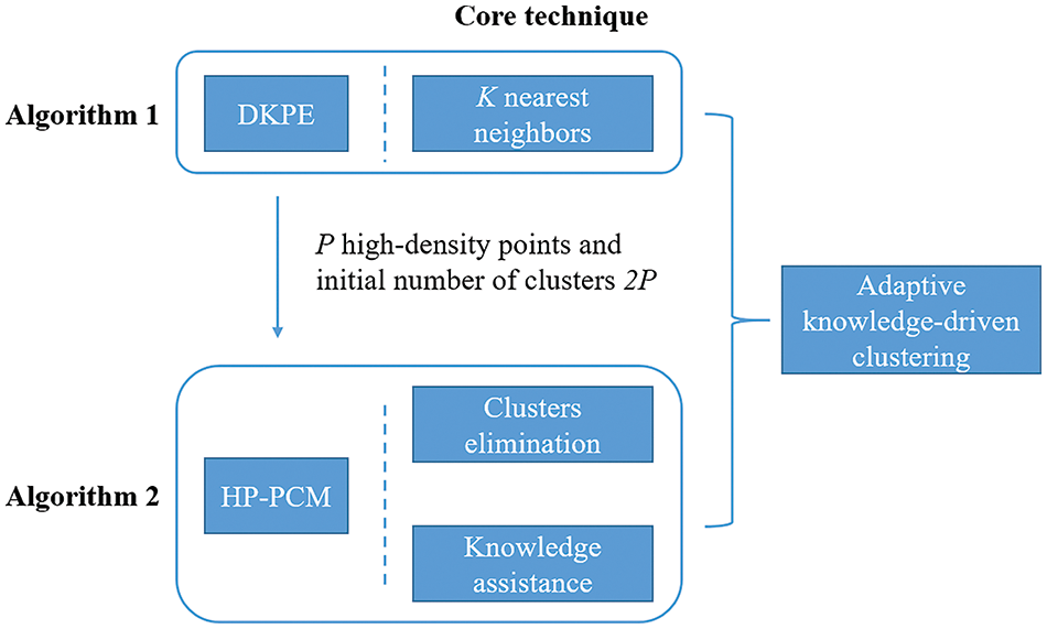
Figure 3: Overall idea of HP-PCM

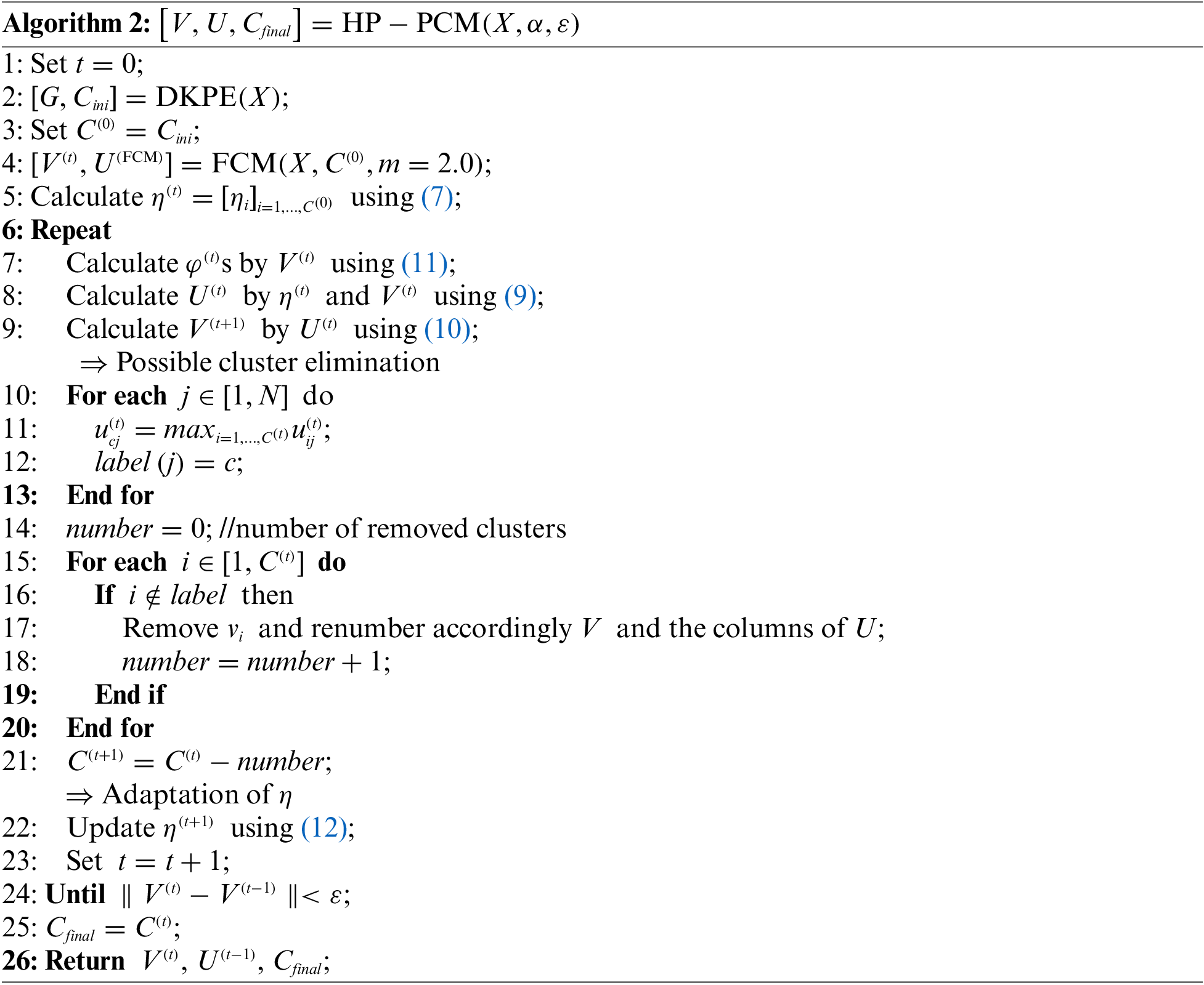
High-density points are the essence of the proposed HP-PCM algorithm because they guide the clustering process to more accurately uncover the latent structure of the dataset. The proposed DKPE algorithm introduced in Section 4.1 can obtain these high-density points. Its specific execution is shown in Algorithm 1. After obtaining high-density points, the HP-PCM algorithm is applied for dataset clustering. The initialization of Cini is another key step in the HP-PCM algorithm. Its value should be larger than the actual cluster numbers. In the experiment in Section 5, we show that the number of high-density points got by the DKPE algorithm closely approximates the actual number of clusters. Therefore, we set Cini to be twice the number of high-density points. See Algorithm 2 for other details.

4.4 Computational Complexity

Given the input dataset with N samples and T iterations, there are three main parts for the computational complexity of HP-PCM. The first part is the knowledge extraction method, DKPE. Its main computational cost is searching the K-nearest neighbors of each sample based on the KD-tree structure. Therefore, the time complexity of DKPE is 𝒪(Nlog⁡(N)). The second part involves the FCM algorithm, which obtains the initial cluster centers and membership degrees. The computational complexity of FCM is 𝒪(NTFCMCini), where TFCM is the iteration number of FCM. The third major part of HP-PCM is the T iterations to update the cluster centers and the membership degree matrix. The computational complexity of this part is 𝒪(NTCini). Thus, the overall cost of HP-PCM is 𝒪(Nlog⁡(N)+NTFCMCini+NTCini).

5  Experiments

To verify the performance of our proposed DKPE algorithm for extracting density knowledge points and the clustering performance of the proposed HP-PCM algorithm, we conduct a series of experiments and analyze the corresponding results.

5.1 Used Datasets and Comparative Algorithms

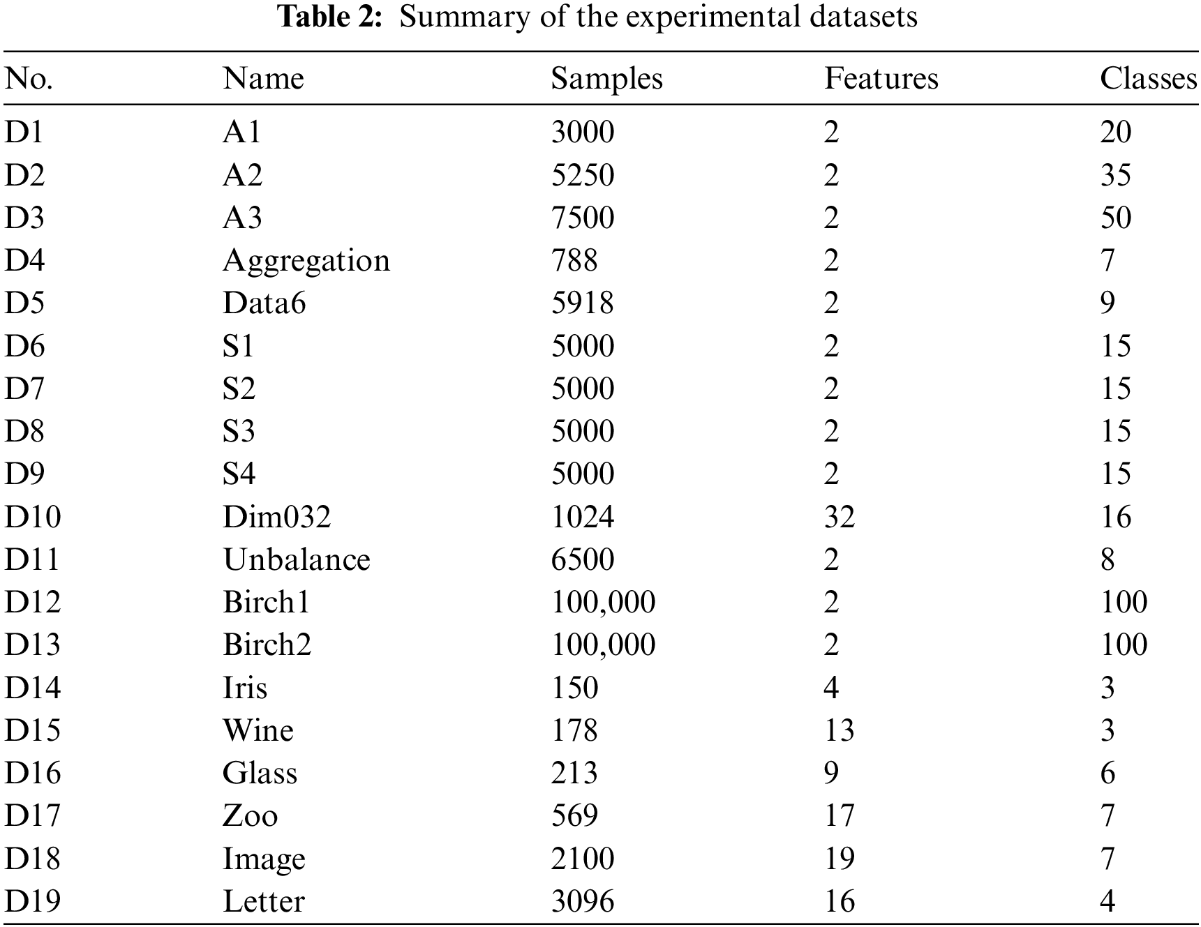
All the information about the datasets used for the experiments, including the total number of samples and the actual number of clusters, is summarized in Table 2. The clustering results for the two-dimensional synthetic datasets visually show the effectiveness of the DKPE and HP-PCM algorithms. Datasets D6 to D13 are mainly used to explore the effects of data dimensionality, structure, size, and other elements on the clustering performance of the proposed HP-PCM algorithm. The UCI datasets (D15 to D19) are used to compare the proposed HP-PCM algorithm with 10 state-of-the-art algorithms across different types, including 1) 3 traditional fuzzy clustering algorithms: FCM, PCM, and PFCM; 2) 2 knowledge-driven fuzzy clustering algorithms: V-FCM and DVPFCM; 3) a density-based clustering algorithm: DPC; 4) 2 advanced possibilistic algorithms: APCM and C-PCM; and 5) 2 clustering algorithms based on performance indices: Silhouette [41] and fRisk4-bA [20]. Among these comparative algorithms, DPC, APCM, Silhouette, and fRisk4-bA are not only used to compare clustering performance but also to evaluate the accuracy and efficiency in determining the number of clusters. The other algorithms are primarily used to compare the performance of clustering models in terms of evaluation metrics, convergence speed, time cost, and adaptability to different datasets. All the used algorithms are implemented by MATLAB R2019b.

5.2 Evaluation Indices

To evaluate clustering results of algorithms, we employ 1) the success rate (SR), which measures the percentage of patterns that are correctly classified, 2) the Normalized Mutual Information (NMI), which is an asymmetric measure to quantify the statistical information shared between two cluster distributions [42], 3) the Adjusted Rand Index (ARI), which evaluates on a pairwise-basis, 4) the Centroid Index (CI), which counts the number of clusters that miss a centroid, or have too many centroids, 5) the Xie-Beni index (XB), which is popular in measuring fuzzy clustering performance [43]. These five indices allow the number of clusters obtained by algorithms to be inconsistent with the reference number. They are described in detail as follows:

1) The Success Rate (SR) measures the percentage of patterns that are correctly classified. This index is calculated as follows:

SR(+)=∑i=1CdiN(13)

where di is the number of objects correctly identified in the ith cluster, and N is the number of all objects in the dataset.

2) The Normalized Mutual Information (NMI) is an asymmetric measure to quantify the statistical information shared between two cluster distributions [42]. The larger such index is, the more similar the two class distribution are and the better the clustering performance is. NMI is calculated as follows:

NMI(+)=∑i=1I∑j=1JP(i,j)log⁡P(i,j)P(i)P(j)(H(R)H(Q))(14)

where R and Q are two partitions of the dataset. Assume that R, Q have I, J clusters, respectively. P(i) denotes the probability of an object belonging to cluster Ri with R partition. More specifically, P(i)=|Ri|N where |Ri| is the number of samples in cluster Ri. P(i,j) denotes the probability that an object belongs to cluster Ri with R partition and cluster Qj with Q partition. P(i,j) is calculated as P(i,j)=|Ri∩Qj|N. H(R) is the entropy associated with all probabilities P(i) in partition R, and H(R)=−∑i=1IP(i)log⁡P(i). The definition of H(Q) is similar to this.

3) The Adjusted Rand Index (ARI), which evaluates on a pairwise-basis. Assuming that R and Q are two hard partitions, here we first introduce some definitions:

a is the number of data point pairs that belong to the same class with R partition and to the same cluster in Q partition simultaneously;

b is the number of data point pairs that belong to the same class in R partition and to different clusters in Q partition simultaneously;

c is the number of data point pairs that belong to different clusters in R partition and to the same cluster in Q partition simultaneously;

d is the number of data point pairs that belong to different clusters in R partition and to different clusters in Q partition simultaneously.

The ARI is defined as follows:

ARI(+)=a−(a+b)(a+c)d(a+b)+(a+c)2−(a+b)(a+c)d.(15)

4) The Centroid Index (CI) counts the number of clusters that miss a centroid, or have too many centroids. Given two sets of prototypes C={c1,c2,…,ck1} and C={c1,c2,…,ck2}, the nearest neighbor mappings (C→C′) are constructed as follows:

qi← 1≤j≤k2argmin∥Ci−C′∥2,∀i∈[1,k1].(16)

Here, we use orphan (cj′) to denote whether it has a prototype that map to the target prototype cj′:

orphan(cj′)={1,qi≠j,∀i0,otherwise(17)

The dissimilarity of C in respect to C′ is the number of orphan prototypes:

CI1(C,C′)=∑j=1k2orphan(Cj′).(18)

The mapping is not symmetric, i.e., C→C′≠C′→C, so CI is defined as:

CI(−)=max{CI1(C,C′),CI1(C′,C)}.(19)

5) The Xie-Beni index (XB) is popular in measuring fuzzy clustering performance [43]. The XB index focuses on compactness and separation, where compactness is a measure of proximity between data points within a cluster and separation is a measure of the distance between one cluster and another cluster. The XB index is defined as follows:

XB(−)=∑i=1C∑j=1Nuijmd(xj,vi)N×mind(vi,vk).(20)

5.3 Test for DKPE

The DPC algorithm also has the capability to acquire high-density points, but it struggles with the challenge of determining the parameter r, as discussed earlier in Section 4.2. The quality of the obtained high-density points depends heavily on the value of r. Therefore, we propose the high-density point extraction method, DKPE, to overcome the parameter sensitivity. To compare the performance of DKPE and DPC in identifying high-density points, we use the A1–A3 datasets from [44]. The A1–A3 datasets are 2-dimensional datasets with an increasing number of clusters (A1: 20, A2: 35, A3: 50), decreasing distances between clusters, and gradually increasing total sample size (A1: 3000, A2: 5250, A3: 7500), which also indicates increasing clustering difficulty.

Fig. 4 shows the experimental results of the DKPE and DPC algorithms on the A1, A2, and A3 datasets. The red dots in Fig. 4d–f mark the high-density points obtained by the proposed DKPE algorithm, and the blue dots of the high-density points distribution graphs in Fig. 4g–i mark the high-density points obtained by the DPC algorithm.

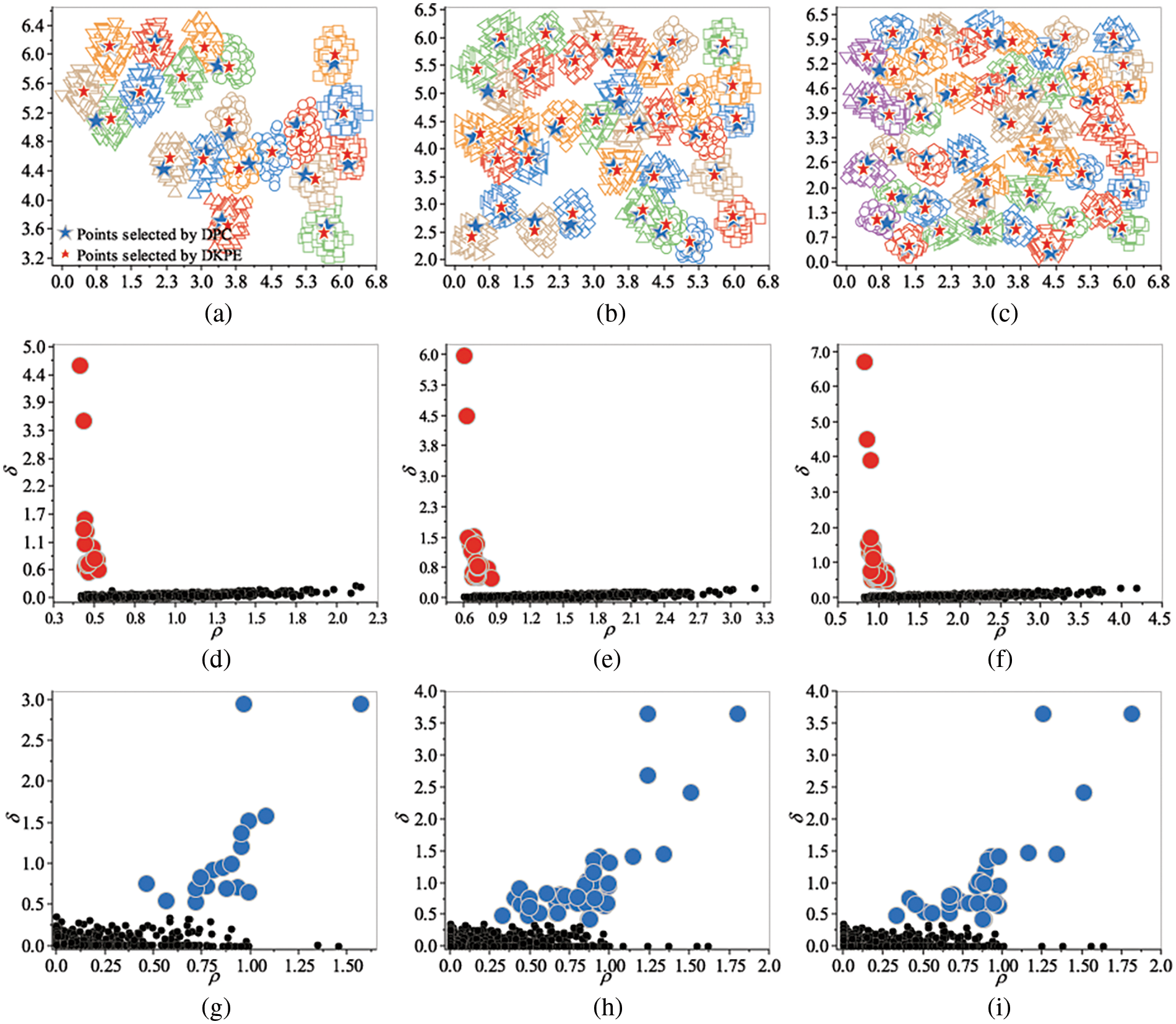
Figure 4: Results on the A1–A3 datasets. (a–c) Data distribution and high-density point distribution of A1, A2, and A3, respectively. Different colors and shapes represent different clusters. (d–f) Decision graph of the DKPE algorithm for A1, A2, and A3, respectively. Red points are selected high-density points by DKPE. (g–i) Decision graph of the DPC algorithm for A1, A2, and A3, respectively. Blue points are selected high-density points by DPC

As shown in Fig. 4d–f, the DKPE algorithm highlights the high-density points, creating a clear distinction between these and non-high-density points (represented as black dots in the decision graphs). This clear separation makes it easy for us to extract the high-density points shown in red. In comparison, there is no obvious boundary between the high-density and the non-high-density points for DPC. Therefore, it is difficult for us to distinguish between high-density and non-high-density points. Focusing on the results shown in Fig. 4a–c, we can see that the number of high-density points obtained by the proposed DKPE algorithm equals the reference number. The extracted high-density points are located in dense district centers. Furthermore, the number of cluster centers obtained by the DPC algorithm is fewer than the reference number of clusters, with some selected cluster centers situated between dense regions, leading to an underestimation of the actual number of clusters. This result shows that the proposed DKPE algorithm can be better applied to datasets with multiple dense regions than the DPC algorithm.

5.4 Parameter Analyses

Next, we investigate the effect of parameter α on the proposed HP-PCM algorithm and its value selection. The datasets A1–A3, Aggregation [45] and Data6 in [46] are used as experimental objects. From Fig. 5a, we can see that Aggregation contains 7 clusters but the size of each cluster is different, so it causes the larger clusters to have more than one high-density point, and the total number of high-density points is 10, lager than the reference number of clusters, 7. That means density-based clustering algorithms may fail in obtaining the optimal number of clusters for an unbalanced dataset. Data6 consists of 918 data points and 5000 noise points. Its reference number of clusters is 9. As shown in Fig. 5b, the number of noises in Data6 is much more than the data points, and the data-intensive areas are not prominent. This data distribution feature is a great challenge for the HP-PCM algorithm to cluster.

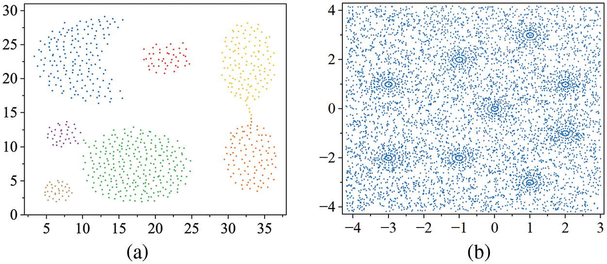
Figure 5: Distribution of Aggregation and Data6. (a) Aggregation. (b) Data6

Fig. 6 shows the influence of the parameter α on the difference between the true number of clusters and the final number of clusters obtained by HP-PCM on each dataset when it changes in the interval [0.1,2]. The difference Cdiff=Ctrue−Cfinal. Cdiff=0 means HP-PCM gets the correct number of clusters. If α takes a value between 0.1 and 0.9, the HP-PCM algorithm is less likely to obtain the ideal Cfinal. When α varies in [1.4,2], the HP-PCM algorithm cannot correctly get the optimal clusters for the A3 dataset. With further comparison, we can find that when the value of α is 1 to 1.3, the proposed HP-PCM algorithm gets all five datasets the correct optimal clusters numbers as Cdiff=0. So, we set α to 1.2 in the previous and next experiments. In addition, the difference in the number of clusters obtained by the HP-PCM algorithm is small throughout the variation, which indicates that the proposed HP-PCM algorithm has a good and stable performance in determining the optimal number of clusters.

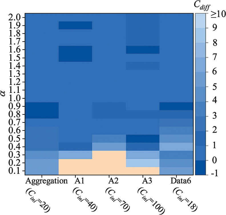
Figure 6: Graphical representation of the difference between the reference number of clusters and the final number of clusters got by HP-PCM on five datasets for various values of α

5.5 Synthetic Datasets

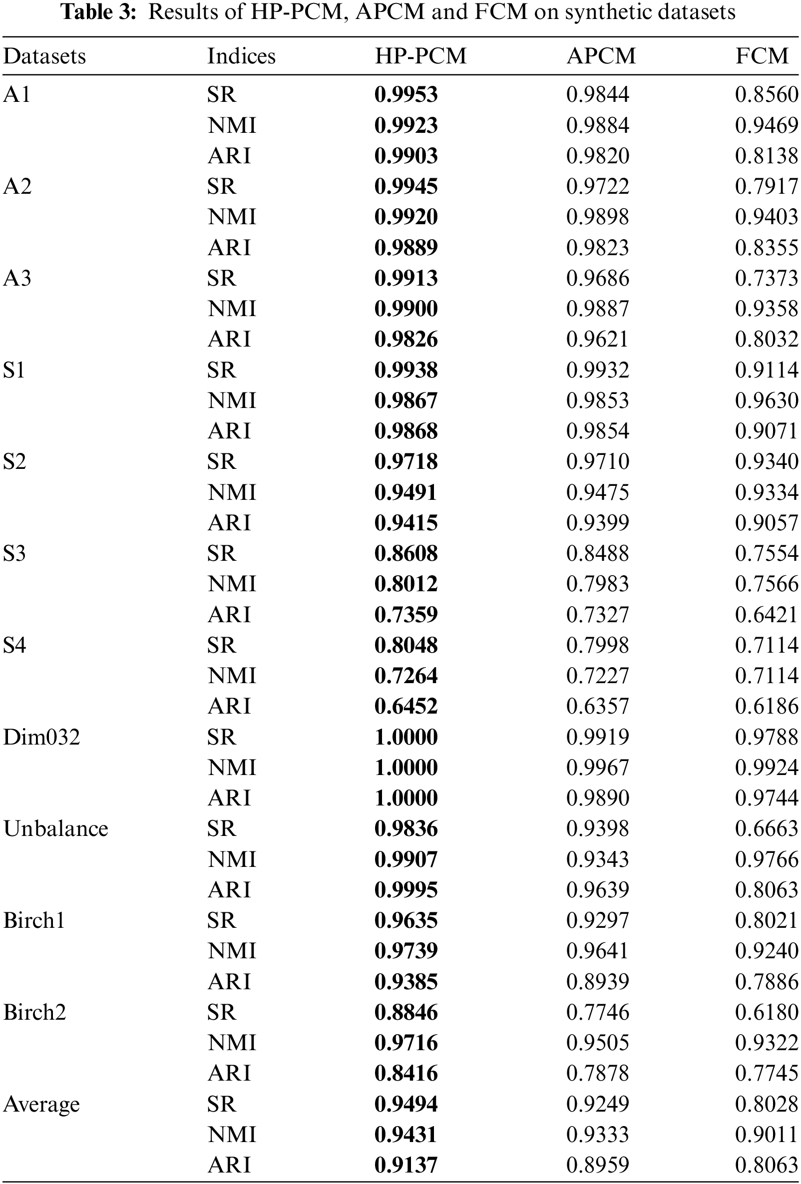
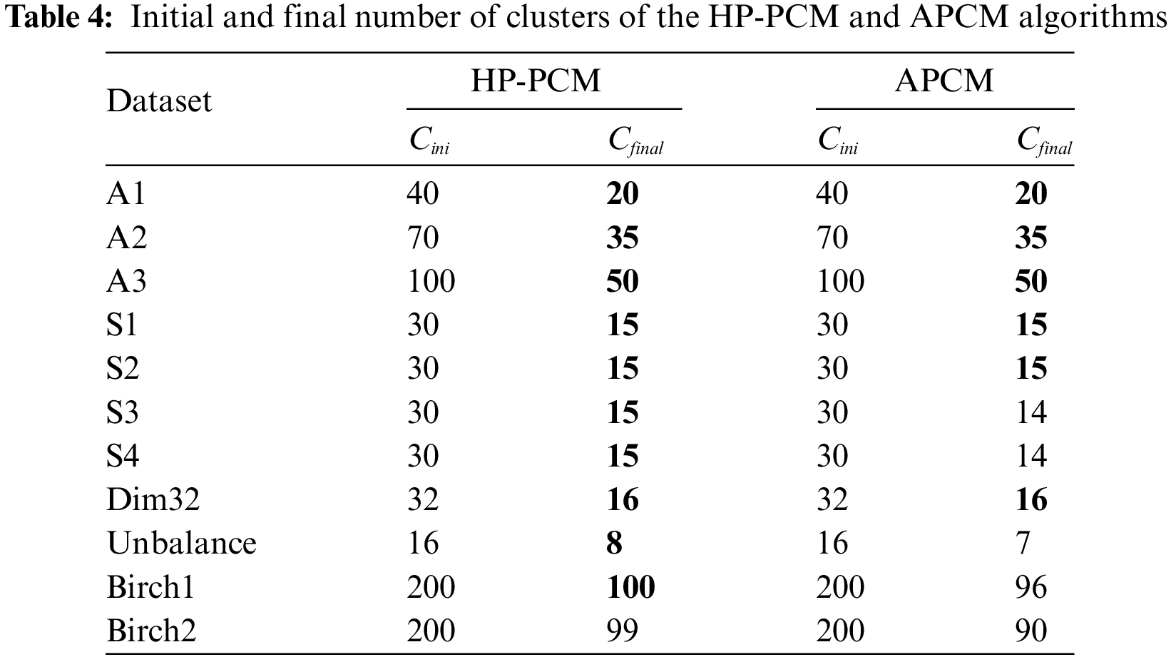
Here, synthetic datasets A1–A3, S1–S4 [47], Dim032 [48], Unbalance [49], Birch1 and Birch2 [50] are used to study the properties of the HP-PCM algorithm and compare with the advanced APCM algorithm and the traditional FCM algorithm. Table 3 summarizes the overall results of HP-PCM, APCM and FCM. We see that the proposed HP-PCM algorithm performs better than the APCM and FCM algorithms on all datasets. On average, the HP-PCM algorithm has 94.94% of success rate which is 2.64% and 18.26% higher than that of the APCM and the FCM algorithm respectively. As can be seen from Table 4, the HP-PCM only failed to obtain the actual clusters on the Birch2 dataset, while the APCM algorithm failed on five datasets which are the S3, S4, Unbalance, Birch1, and Birch2 datasets. We next analyze the results in more detail from two aspects: the size of samples and the number of clusters.

The A1–A3 datasets have an increasing number of clusters, ranging from 20 to 50. From Table 3, we can see that the values of SR, NMI, and ARI decrease for all three algorithms as the number of clusters increases. Moreover, Fig. 7 demonstrates how the CI-value depends on the size of the data (Fig. 7a), and on the number of clusters (Fig. 7b) for the HP-PCM, APCM, and FCM algorithms. The value of CI fluctuates as the size of the data changes and it seems that there is no clear dependency on the size of the data for the three algorithms. On average, the value of CI for the HP-PCM algorithm is 13.92, compared to 17.54 and 18.29 for the APCM and FCM algorithms, respectively, indicating that HP-PCM performs slightly better. This improved performance of the HP-PCM algorithm can be attributed to its ability to produce a final number of clusters that is closer to, or even equal to, the actual number of clusters, whereas the APCM algorithm consistently identifies fewer clusters across all Birch2 subsets (as shown in Fig. 8a). In general, the values of CI for all algorithms increase almost linearly along with the increasing number of clusters (see Fig. 7b). This suggests that as the number of clusters grows, the difference between the cluster centers obtained by the algorithms and the ground truth centroids also increases. As illustrated in Figs. 7b and 8b, when the number of clusters is less than 24, the HP-PCM algorithm can get correct number of clusters, resulting in a CI value of zero, which matches the ground truth centroids. For the APCM algorithm, when the number of clusters is over 16, it obtains fewer clusters than the actual number, leading to a higher value of CI than that of the HP-PCM algorithm. Overall, increasing the number of clusters will degrade the performance of HP-PCM, APCM, and FCM algorithms.

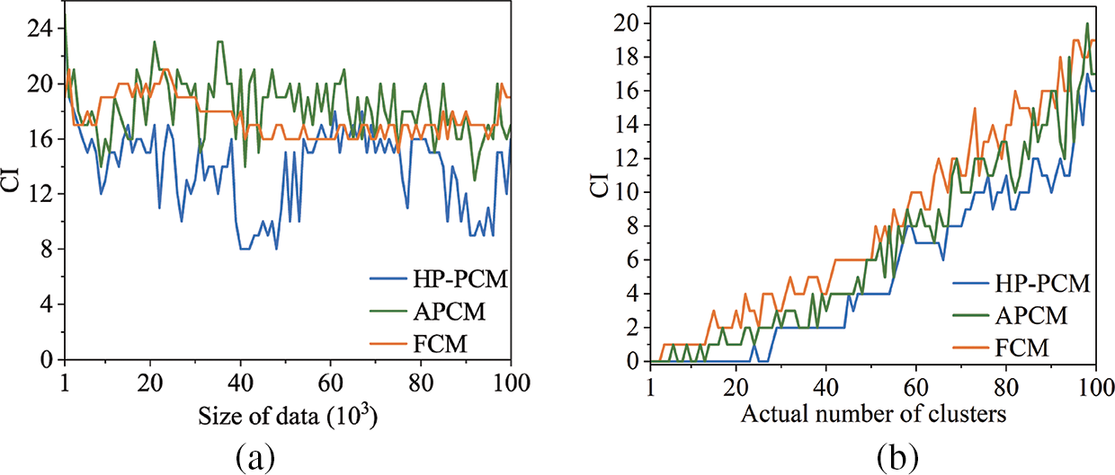
Figure 7: Dependency of the values of CI on the size of data (Birch2-random), and on the number of clusters (Birch2-sub)

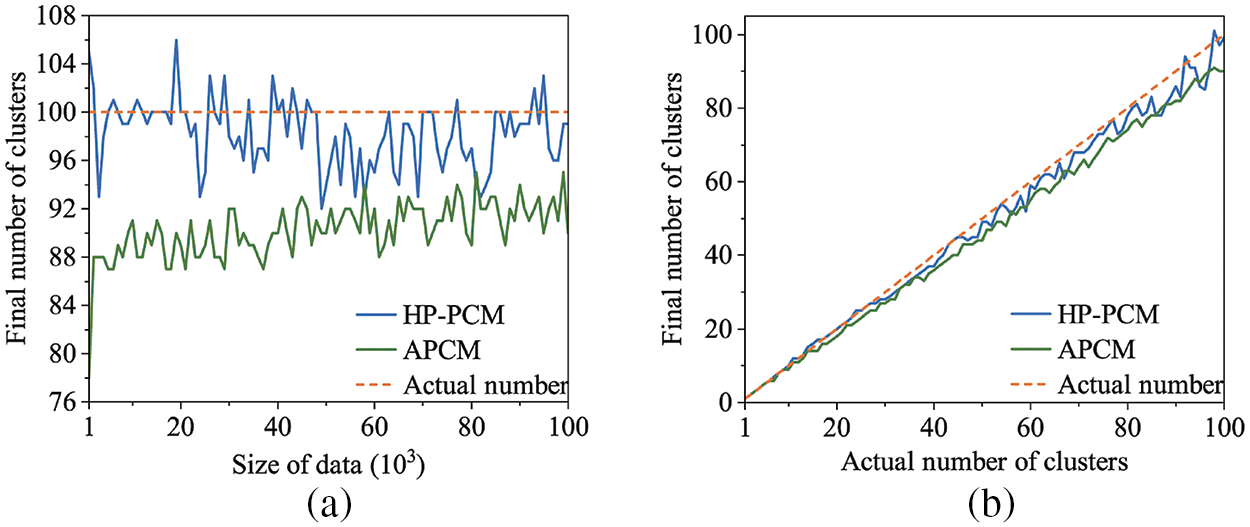
Figure 8: Dependency of the number of the final clusters on the size of data (Birch2-random), and on the number of clusters (Birch2-sub)

5.6 UCI Datasets

Next, we compare the clustering results of the proposed HP-PCM algorithm with ten state-of-the-art algorithms: FCM, PCM, PFCM, V-FCM, Silhouette, DPC, APCM, C-PCM, DVPFCM, and fRisk4-bA. The characteristics of the adopted UCI datasets [51] are shown in Table 2. The index values for FCM, PCM, PFCM, V-FCM, APCM, C-PCM, and HP-PCM are the best values after running 20 times.

Tables 6–8 present the performance index values (SR, NMI, XB) obtained by 11 clustering algorithms on the selected machine learning datasets, respectively. The best results are highlighted in bold. Since DPC and Silhouette belong to hard clustering algorithms, they do not have XB values.

Cini and Cfinal in Table 5 represent the initial and final cluster number of a clustering algorithm, respectively.

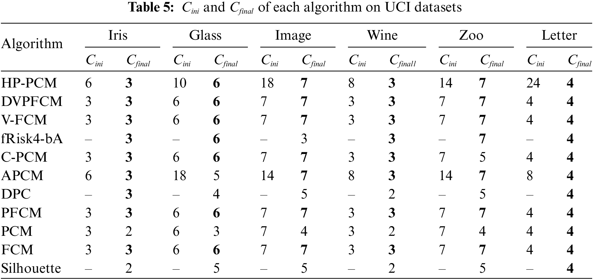
Tables 6–8 show that the proposed HP-PCM algorithm outperforms the other comparative algorithms across all evaluation metrics. Table 5 shows that HP-PCM can always obtain the same number of final clusters as the true number of clusters. For the four datasets, Wine, Glass, Image, and Letter, the number of high-density points identified by the DKPE method is higher than the actual number of clusters, especially for the image dataset, where the 24 high-density points are identified compared to the correct number of 4 clusters. However, our proposed HP-PCM algorithm still accurately determines the final number of clusters and ensures that the clustering results are better. This is due to the parameter φ in the HP-PCM algorithm, which regulates the influence of knowledge points, enhancing the guidance provided by true high-density points while diminishing the misleading effects of non-high-density points. As a result, guided by the high-density points, the HP-PCM algorithm can obtain more desirable clustering results.

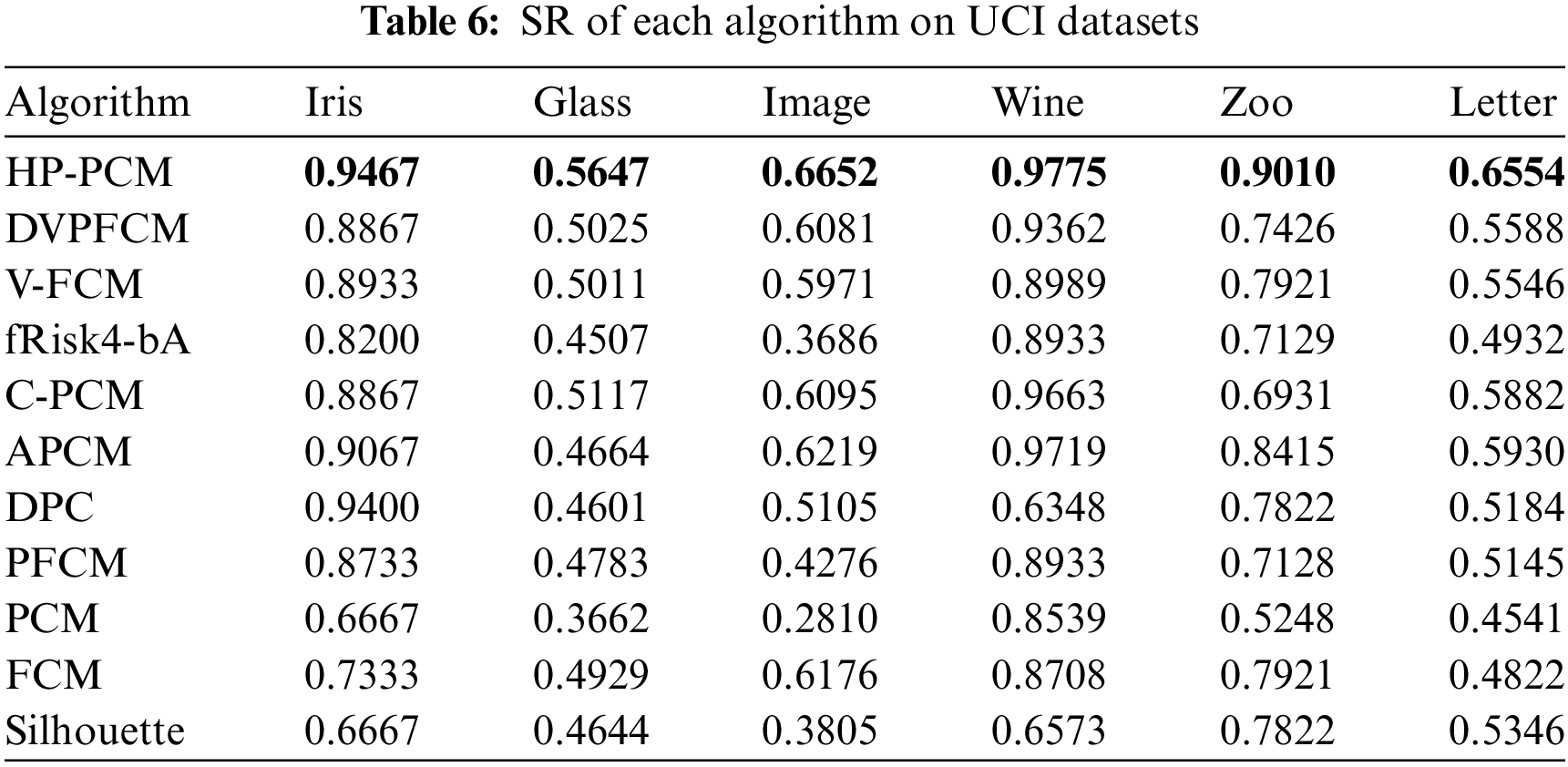
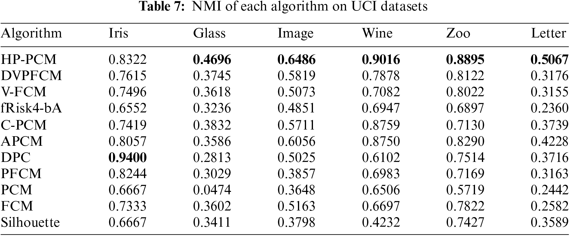
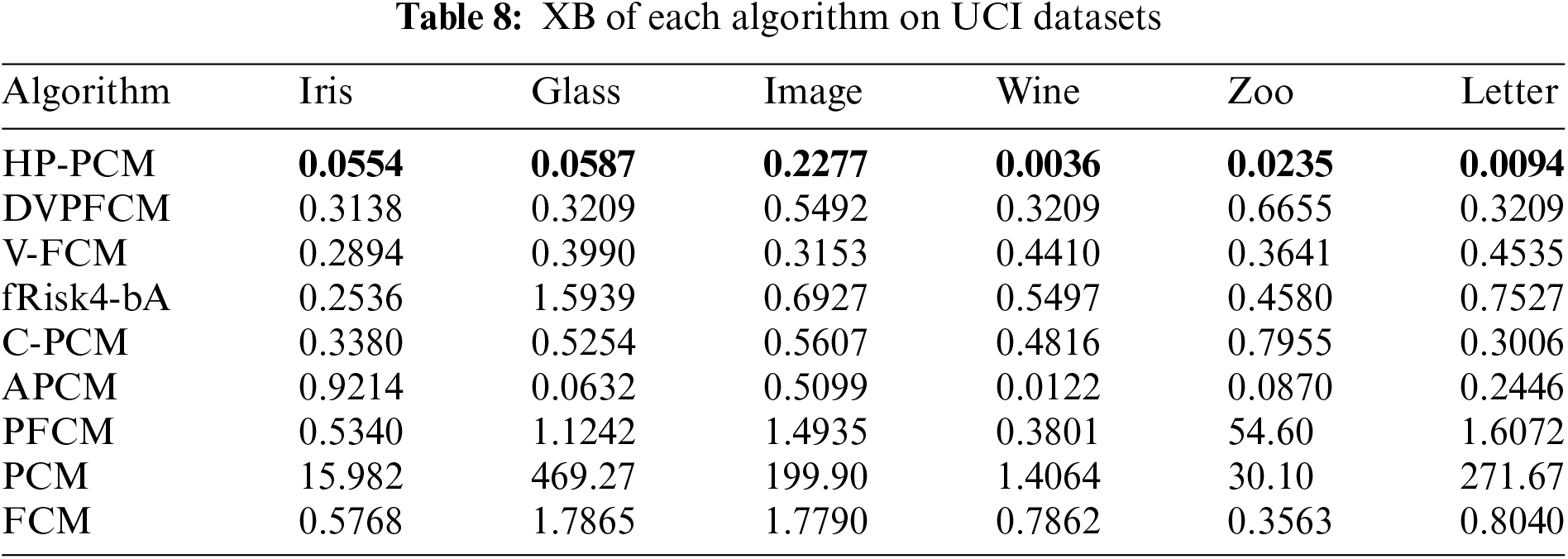
Both the fRisk4-bA and Silhouette algorithms determine the optimal number of clusters based on the evaluation index values. fRisk4-bA can accurately obtain the optimal number of clusters (except for the Image dataset), but its SR and NMI values are not higher than those of the other algorithms, and its XB value is not less. This is because fRisk4-bA uses FCM to obtain the clustering results but FCM is sensitive to noises. For the Silhouette algorithm, the main reason for its poorer clustering performance is that it fails to correctly determine the optimal number of clusters.

The final number of clusters obtained by PCM tends to be smaller than the actual number of clusters on the Iris, Wine, Zoo, and Image datasets, likely due to the influence of clustering center uniformity. The knowledge-based clustering algorithms DVPFCM and V-FCM replace one of the final cluster centers with the highest-density point, so their performance is better than that of the FCM, PCM, PFCM algorithms and even better than that of CPCM, and APCM on some datasets. However, their clustering flexibility is constrained by the highest-density point. When the obtained highest-density point is not the true high-density point, DVPFCM and V-FCM may obtain misleading clustering results. Consequently, their clustering performance is not always better than that of the CPCM and APCM algorithms.

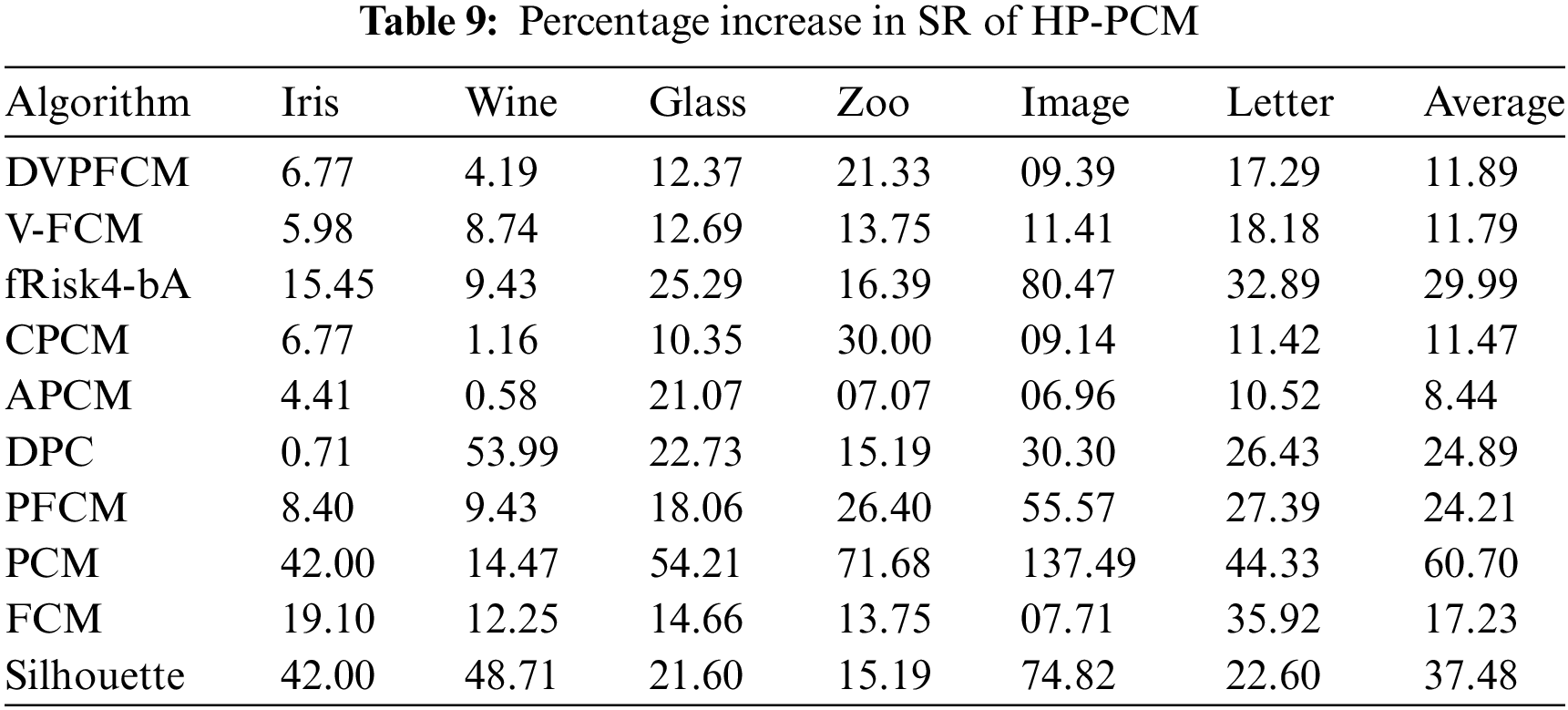
To further illustrate the performance improvement of the proposed HP-PCM algorithm, we counted the percentage increase in SR of the HP-PCM algorithm relative to the compared algorithms, as shown in Table 9. From Table 9, we can see that HP-PCM has at most a 137.49% improvement in the clustering success rate. On average, the HP-PCM algorithm can improve SR by 8.44% and up to 60.70% relative to the other algorithms.

In addition, Fig. 9 counts the number of iterations required for each clustering algorithm on the six used UCI datasets. The fRisk4-bA, DPC, and Silhouette algorithms are not iterative, so they are not considered with this statistic. It can be seen from Fig. 9 that the proposed HP-PCM algorithm requires the fewest iterations, followed by the DVPFCM and V-FCM algorithms. This suggests that the introduction of knowledge hints can help speed up the algorithm convergence.

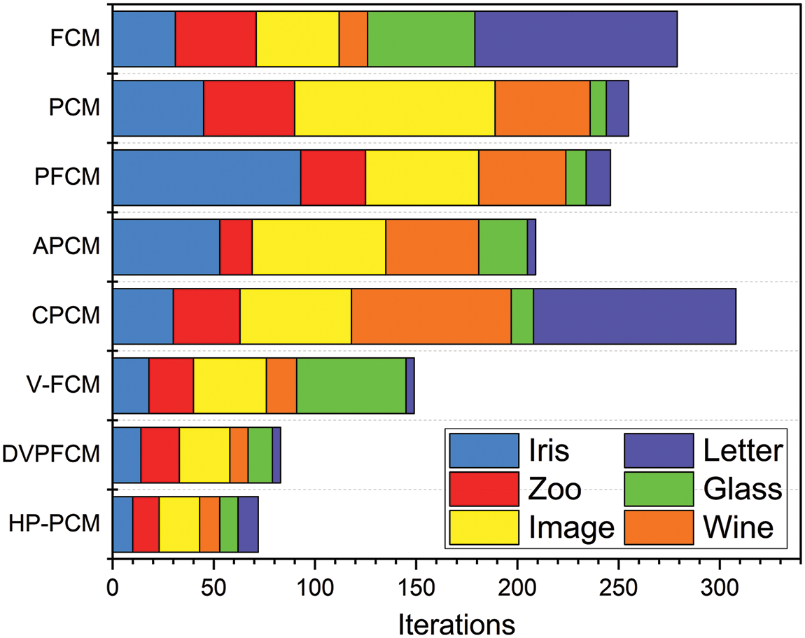
Figure 9: Average numbers of iteration for the tested algorithms

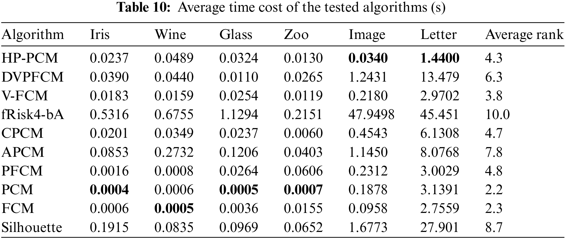
Table 10 summarizes the average running time of the tested algorithms on the used UCI datasets. It is evident that the Silhouette and fRisk4bA algorithms are the slowest among all algorithms. This slow performance highlights the significant time requirements for determining the number of clusters and analyzing dataset structure using clustering indices. In contrast, the HP-PCM algorithm shows markedly better time efficiency compared to other algorithms designed for identifying the optimal number of clusters, including Silhouette, APCM, and fRisk4-bA.

Overall, HP-PCM is the best in terms of various performance indices and the required number of iterations.

5.7 Ablation Study

Comparing the above clustering results of the proposed HP-PCM algorithm and the APCM algorithm, we can observe that high-density points help the algorithm to determine the final number of clusters more accurately and efficiently. To reveal the impact of high-density points on the adaptive determination of the number of clusters, we designed four algorithms and compared their performance. The first algorithm, denoted as Ablation 1, replaces high-density points with a randomly sampled set of points from the dataset. The second algorithm, denoted as Ablation 2, obtains high-density points from the DPC algorithm. The third algorithm, denoted as Ablation 3, is our proposed HP-PCM algorithm, which uses high-density points provided by the DKPE algorithm. The results of these three algorithms on the six UCI datasets are shown in Table 11. Table 11 demonstrates that Ablation 3, the HP-PCM algorithm, outperforms Ablation 2 and Ablation 1 in terms of SR and NMI across all UCI datasets. Furthermore, Ablation 2 outperforms Ablation 1 on five out six datasets with respect to SR and NMI. In conclusion, the ablation experimental results clearly indicate that high-density points play a crucial role in enhancing the accuracy and efficiency of clustering algorithms.

6  Conclusion

In this study, we propose a novel knowledge-driven clustering algorithm called the HP-PCM algorithm. First, the DKPE method is proposed to obtain P data points with higher density. Then, these high-density points are added to the objective function of PCM to construct a new function, which is the HP-PCM algorithm objective function. In the HP-PCM algorithm, the high-density points serve as guides, rather than deciders, facilitating the algorithm to find dense regions within the dataset. Furthermore, the proposed HP-PCM algorithm can automatically and accurately determine the final number of clusters by employing the cluster merging mechanisms. Finally, compared with 10 existing clustering algorithms on different datasets, the experimental results show that our proposed HP-PCM algorithm is better at determining the initial number of clusters, getting the success rate of clustering, and obtaining the optimal number of clusters. By comparing the number of iterations, it is shown that the knowledge-driven clustering algorithms DVPFCM, V-FCM, and our proposed HP-PCM algorithms have fewer iterations, which fully shows that the high-density points help speed up the algorithm convergence.

Our future work will focus on the extension of HP-PCM to cluster the datasets with irregular shapes. Moreover, it would be helpful to combine fuzzy clustering with fuzzy inference [52].

Acknowledgement: Special thanks to the reviewers of this paper for their valuable feedback and constructive suggestions, which greatly contributed to the refinement of this research.

Funding Statement: This work was supported by the National Key Research and Development Program of China (No. 2022YFB3304400) and the National Natural Science Foundation of China (Nos. 6230311, 62303111, 62076060, 61932007, and 62176083), and the Key Research and Development Program of Jiangsu Province of China (No. BE2022157).

Author Contributions: The authors confirm contribution to the paper as follows: study conception and design: Xianghui Hu, Yichuan Jiang; data collection: Yiming Tang; analysis and interpretation of results: Xianghui Hu, Witold Pedrycz, Jiuchuan Jiang; draft manuscript preparation: Xianghui Hu, Yiming Tang, Jiuchuan Jiang. All authors reviewed the results and approved the final version of the manuscript.

Availability of Data and Materials: All the synthetic datasets used in this article are sourced from “Dynamic local search for clustering with unknown number of clusters” [44], “Clustering aggregation” [45], “Generalized entropy based possibilistic fuzzy c-means for clustering noisy data and its convergence proof” [46], “Iterative shrinking method for clustering problems” [47], “Fast agglomerative clustering using a k-nearest neighbor graph” [48], “Set-matching methods for external cluster validity” [49], “BIRCH: A new data clustering algorithm and its applications” [50]; all the UCI datasets used in this article are available from: https://archive.ics.uci.edu/ (accessed on 20 May 2024).

Ethics Approval: Not applicable.

Conflicts of Interest: The authors declare that they have no conflicts of interest to report regarding the present study.

References

1. F. Fontana, C. Klahn, and M. Meboldt, “Value-driven clustering of industrial additive manufacturing applications,” Int. J. Manuf. Technol. Manag., vol. 30, no. 2, pp. 366–390, Feb. 2019. doi: 10.1108/JMTM-06-2018-0167. [Google Scholar] [CrossRef]

2. H. Y. Li, B. Zhang, S. Qin, and J. L. Peng, “UAV-Clustering: Cluster head selection and update for UAV swarms searching with unknown target location,” presented at the WoWMoM, Belfast, UK, Jun. 14–17, 2022, pp. 483–488, doi: 10.1109/WoWMoM54355.2022.00075. [Google Scholar] [CrossRef]

3. Y. M. Tang, F. J. Ren, and W. Pedrycz, “Fuzzy C-Means clustering through SSIM and patch for image segmentation,” Appl. Soft Comput., vol. 87, no. 4, Feb. 2020, Art. no. 105928. doi: 10.1016/j.asoc.2019.105928. [Google Scholar] [CrossRef]

4. F. Liu, L. C. Jiao, and X. Tang, “Task-oriented GAN for PolSAR image classification and clustering,” IEEE Trans. Neural Netw. Learn. Syst., vol. 30, no. 9, pp. 2707–2719, Sep. 2019. doi: 10.1109/TNNLS.2018.2885799. [Google Scholar] [PubMed] [CrossRef]

5. P. Fränti, M. Rezaei, and Q. P. Zhao, “Centroid index: Cluster level similarity measure,” Pattern Recognit., vol. 47, no. 9, pp. 3034–3045, Sep. 2014. doi: 10.1016/j.patcog.2014.03.017. [Google Scholar] [CrossRef]

6. J. C. Dunn, “A fuzzy relative of the ISODATA process and its use in detecting compact well-separated clusters,” J. Cybern., vol. 3, no. 3, pp. 32–57, Sep. 1973. doi: 10.1080/01969727308546046. [Google Scholar] [CrossRef]

7. J. C. Bezdek, “Objective function clustering,” in Pattern Recognition with Fuzzy Objective Function Algorithms, 1st ed., New York, NY, USA: Springer, 2013, pp. 65–79, doi: 10.1007/978-1-4757-0450-1_3. [Google Scholar] [CrossRef]

8. A. Bagherinia, M. B. Behrooz, H. Mehdi, and H. Parvin, “Reliability-based fuzzy clustering ensemble,” Fuzzy Sets Syst., vol. 413, pp. 1–28, Jun. 2021. doi: 10.1016/j.fss.2020.03.008. [Google Scholar] [CrossRef]

9. H. Li and M. Wei, “Fuzzy clustering based on feature weights for multivariate time series,” Knowl.-Based Syst., vol. 197, no. 8, Jun. 2020, Art. no. 105907. doi: 10.1016/j.knosys.2020.105907. [Google Scholar] [CrossRef]

10. S. D. Xenaki, K. D. Koutroumbas, and A. A. Rontogiannis, “A novel adaptive possibilistic clustering algorithm,” IEEE Trans. Fuzzy Syst., vol. 24, no. 4, pp. 791–810, Aug. 2016. doi: 10.1109/TFUZZ.2015.2486806. [Google Scholar] [CrossRef]

11. S. D. Xenaki, K. D. Koutroumbas, and A. A. Rontogiannis, “Sparsity-aware possibilistic clustering algorithms,” IEEE Trans. Fuzzy Syst., vol. 24, no. 6, pp. 1611–1626, Dec. 2016. doi: 10.1109/TFUZZ.2016.2543752. [Google Scholar] [CrossRef]

12. W. Pedrycz, V. Loia, and S. Senatore, “Fuzzy clustering with viewpoints,” IEEE Trans. Fuzzy Syst., vol. 18, no. 2, pp. 274–284, Apr. 2010. doi: 10.1109/TFUZZ.2010.2040479. [Google Scholar] [CrossRef]

13. Y. M. Tang, X. H. Hu, W. Pedrycz, and X. C. Song, “Possibilistic fuzzy clustering with high-density viewpoint,” Neurocomputing, vol. 329, no. 2, pp. 407–423, Feb. 2019. doi: 10.1016/j.neucom.2018.11.007. [Google Scholar] [CrossRef]

14. Y. M. Tang, Z. F. Pan, X. H. Hu, W. Pedrycz, and R. H. Chen, “Knowledge-induced multiple kernel fuzzy clustering,” IEEE Trans. Pattern Anal. Mach. Intell., vol. 45, no. 12, pp. 14838–14855, Dec. 2023. doi: 10.1109/TPAMI.2023.3298629. [Google Scholar] [PubMed] [CrossRef]

15. X. H. Hu, Y. M. Tang, W. Pedrycz, K. Di, J. C. Jiang, and Y. C. Jiang, “Fuzzy clustering with knowledge extraction and granulation,” IEEE Trans. Fuzzy Syst., vol. 31, no. 4, pp. 1098–1112, Apr. 2023. doi: 10.1109/TFUZZ.2022.3195033. [Google Scholar] [CrossRef]

16. W. Dai, Q. Yang, G. R. Xue, and Y. Yu, “Self-taught clustering,” presented at the ICML, Helsinki, Finland, Jul. 5–9, 2008, pp. 200–207. doi: 10.1145/1390156.1390182. [Google Scholar] [CrossRef]

17. W. H. Jiang and F. L. Chung, “Transfer spectral clustering,” in Proc. Joint Eur. Conf. Mach. Learn. Knowl. Discov. Databases, Berlin, Heidelberg, 2012, vol. 7524, pp. 789–803. doi: 10.1007/978-3-642-33486-3. [Google Scholar] [CrossRef]

18. Z. H. Deng, Y. Z. Jiang, F. L. Chung, H. Ishibuchi, K. S. Choi, and S. T. Wang, “Transfer prototype-based fuzzy clustering,” IEEE Trans. Fuzzy Syst., vol. 24, no. 5, pp. 1210–1232, Oct. 2016. doi: 10.1109/TFUZZ.2015.2505330. [Google Scholar] [CrossRef]

19. A. E. Ezugwu et al., “A comprehensive survey of clustering algorithms: State-of-the-art machine learning applications, taxonomy, challenges, and future research prospects,” Eng Appl. Artif. Intell., vol. 110, Apr. 2022. doi: 10.1016/j.engappai.2022.104743. [Google Scholar] [CrossRef]

20. S. D. Nguyen, V. S. T. Nguyen, and N. T. Pham, “Determination of the optimal number of clusters: A fuzzy-set based method,” IEEE Trans. Fuzzy Syst., vol. 30, no. 9, pp. 3514–3526, Sep. 2022. doi: 10.1109/TFUZZ.2021.3118113. [Google Scholar] [CrossRef]

21. Y. M. Tang, J. J. Huang, W. Pedrycz, B. Li, and F. J. Ren, “A fuzzy clustering validity index induced by triple center relation,” IEEE Trans. Cybern., vol. 53, no. 8, pp. 5024–5036, Aug. 2023. doi: 10.1109/TCYB.2023.3263215. [Google Scholar] [PubMed] [CrossRef]

22. N. Wiroonsri, “Clustering performance analysis using a new correlation-based cluster validity index,” Pattern Recogn., vol. 145, no. 6, Jan. 2024, Art. no. 109910. doi: 10.1016/j.patcog.2023.109910. [Google Scholar] [CrossRef]

23. D. Jollyta, S. Efendi, M. Zarlis, and H. Mawengkang, “Analysis of anoptimal cluster approach: A review paper,” J. Phys.: Conf. Ser., vol. 2421, no. 1, 2023, Art. no. 012015. doi: 10.1088/1742-6596/2421/1/012015. [Google Scholar] [CrossRef]

24. A. Rodriguez and A. Laio, “Clustering by fast search and find of density peaks,” Science, vol. 344, no. 6191, pp. 1492–1496, Jun. 2014. doi: 10.1126/science.1242072. [Google Scholar] [CrossRef]

25. T. Qiu and Y. Li, “Fast LDP-MST: An efficient density-peak-based clustering method for large-size datasets,” IEEE Trans Knowl. Data Eng, vol. 35, no. 5, pp. 4767–4780, May 2023. doi: 10.1109/TKDE.2022.3150403. [Google Scholar] [CrossRef]

26. D. Cheng, Y. Li, S. Xia, G. Wang, J. Huang and S. Zhang, “A fast granular-ball-based density peaks clustering algorithm for large-scale data,” IEEE Trans. Neural Netw. Learn. Syst., pp. 1–14, 2023. doi: 10.1109/TNNLS.2023.3300916. [Google Scholar] [PubMed] [CrossRef]

27. J. S. Zhang and Y. W. Leung, “Improved possibilistic C-means clustering algorithms,” IEEE Trans. Fuzzy Syst., vol. 12, no. 2, pp. 209–217, Apr. 2004. doi: 10.1109/TFUZZ.2004.825079. [Google Scholar] [CrossRef]

28. M. Barni, V. Cappellini, and A. Mecocci, “Comments on a possibilistic approach to clustering,” IEEE Trans. Fuzzy Syst., vol. 4, no. 3, pp. 393–396, Aug. 1996. doi: 10.1109/91.531780. [Google Scholar] [CrossRef]

29. H. Timm, C. Borgelt, C. Döring, and R. Kruse, “An extension to possibilistic fuzzy cluster analysis,” Fuzzy Set Syst, vol. 147, no. 1, pp. 3–16, Oct. 2004. doi: 10.1016/j.fss.2003.11.009. [Google Scholar] [CrossRef]

30. N. R. Pal, K. Pal, J. M. Keller, and J. C. Bezdek, “A possibilistic fuzzy c-means clustering algorithm,” IEEE Trans. Fuzzy Syst., vol. 13, no. 4, pp. 517–530, Aug. 2005. doi: 10.1109/TFUZZ.2004.840099. [Google Scholar] [CrossRef]

31. M. S. Yang and J. B. M. Benjamin, “Sparse possibilistic c-means clustering with Lasso,” Pattern Recogn., vol. 138, Jun. 2023, Art. no. 109348. doi: 10.1016/j.patcog.2023.109348. [Google Scholar] [CrossRef]

32. C. Wu and X. Zhang, “A self-learning iterative weighted possibilistic fuzzy c-means clustering via adaptive fusion,” Expert Syst. Appl., vol. 209, no. 1, Dec. 2022, Art. no. 118280. doi: 10.1016/j.eswa.2022.118280. [Google Scholar] [CrossRef]

33. M. S. Yang and K. L. Wu, “A similarity-based robust clustering method,” IEEE Trans. Pattern Anal. Mach. Intell., vol. 26, no. 4, pp. 434–448, Apr. 2004. doi: 10.1109/TPAMI.2004.1265860. [Google Scholar] [PubMed] [CrossRef]

34. M. S. Yang and C. Y. Lai, “A robust automatic merging possibilistic clustering method,” IEEE Trans. Fuzzy Syst., vol. 19, no. 1, pp. 26–41, Feb. 2011. doi: 10.1109/TFUZZ.2010.2077640. [Google Scholar] [CrossRef]

35. Y. Y. Liao, K. X. Jia, and Z. S. He, “Similarity measure based robust possibilistic c-means clustering algorithms,” J. Convergence Inf. Technol., vol. 6, no. 12, pp. 129–138, Dec. 2011. doi: 10.4156/jcit.vol6.issue12.17. [Google Scholar] [CrossRef]

36. J. V. de Oliveira and W. Pedrycz, “Relational fuzzy clustering,” in Advances in Fuzzy Clustering and its Applications, 1st ed. Chichester, England: John Wiley & Sons Ltd., 2007, pp. 38–40. doi: 10.1002/9780470061190. [Google Scholar] [CrossRef]

37. S. B. Zhou, Z. Y. Xu, and F. Liu, “Method for determining the optimal number of clusters based on agglomerative hierarchical clustering,” IEEE Trans. Neural Netw. Learn. Syst., vol. 28, no. 12, pp. 3007–3017, Dec. 2017. doi: 10.1109/TNNLS.2016.2608001. [Google Scholar] [PubMed] [CrossRef]

38. N. R. Pal and J. C. Bezdek, “On cluster validity for the fuzzy c-means model,” IEEE Trans. Fuzzy Syst., vol. 3, no. 3, pp. 370–379, Aug. 1995. doi: 10.1109/91.413225. [Google Scholar] [CrossRef]

39. J. C. Bezdek and N. R. Pal, “Some new indexes of cluster validity,” IEEE Trans. Syst. Man Cybern B-Cybern, vol. 28, no. 3, pp. 301–315, Jun. 1998. doi: 10.1109/3477.678624. [Google Scholar] [PubMed] [CrossRef]

40. J. L. Bentley, “Multidimensional binary search trees used for associative searching,” Commun. ACM, vol. 9, no. 18, pp. 509–517, Sep. 1975. doi: 10.1145/361002.361007. [Google Scholar] [CrossRef]

41. P. J. Rousseeuw, “Silhouettes: A graphical aid to the interpretation and validation of cluster analysis,” J. Comput. Appl. Math., vol. 20, pp. 53–65, 1987. doi: 10.1016/0377-0427(87)90125-7. [Google Scholar] [CrossRef]

42. A. Strehl and J. Ghosh, “Cluster ensembles—A knowledge reuse framework for combining multiple partitions,” J. Mach. Learn. Res., vol. 3, no. 3, pp. 583–617, 2002. doi: 10.1162/153244303321897735. [Google Scholar] [CrossRef]

43. X. L. Xie and G. Beni, “A validity measure for fuzzy clustering,” IEEE Trans. Pattern Anal. Mach. Intell., vol. 13, no. 8, pp. 841–847, Aug. 1991. doi: 10.1109/34.85677. [Google Scholar] [CrossRef]

44. I. Kärkkäinen and P. Fränti, “Dynamic local search for clustering with unknown number of clusters,” in Proc. Int. Conf. Pattern Recogn., Quebec City, QC, Canada, 2002, vol. 2, pp. 240–243. doi: 10.1109/ICPR.2002.1048283. [Google Scholar] [CrossRef]

45. A. Gionis, H. Mannila, and P. Tsaparas, “Clustering aggregation,” in Proc. Int. Conf. Data Eng., Tokyo, Japan, 2005, vol. 1, no. 1, pp. 341–352. doi: 10.1109/ICDE.2005.34. [Google Scholar] [CrossRef]

46. S. Askari, N. Montazerin, M. F. Zarandi, and E. Hakimi, “Generalized entropy based possibilistic fuzzy c-means for clustering noisy data and its convergence proof,” Neurocomputing, vol. 219, no. 2–3, pp. 186–202, Jan. 2017. doi: 10.1016/j.neucom.2016.09.025. [Google Scholar] [CrossRef]

47. P. Fränti and I. Virmajoki, “Iterative shrinking method for clustering problems,” Pattern Recogn., vol. 39, no. 5, pp. 761–775, May 2006. doi: 10.1016/j.patcog.2005.09.012. [Google Scholar] [CrossRef]

48. P. Fränti, O. Virmajoki, and V. Hautamäki, “Fast agglomerative clustering using a k-nearest neighbor graph,” IEEE Trans. Pattern Anal. Mach. Intell., vol. 28, no. 11, pp. 1875–1881, Nov. 2006. doi: 10.1109/TPAMI.2006.227. [Google Scholar] [PubMed] [CrossRef]

49. M. Rezaei and P. Fränti, “Set-matching methods for external cluster validity,” IEEE Trans. Knowl. Data Eng, vol. 28, no. 8, pp. 2173–2186, Aug. 2016. doi: 10.1109/TKDE.2016.2551240. [Google Scholar] [CrossRef]

50. T. Zhang, R. Ramakrishnan, and M. Livny, “BIRCH: A new data clustering algorithm and its applications,” Data Min. Knowl. Discov., vol. 1, no. 2, pp. 141–182, 1997. doi: 10.1023/A:1009783824328. [Google Scholar] [CrossRef]

51. D. Dua and C. Graff, “UCI machine learning repository,” Accessed: May 20, 2024, Jan. 2017. [Online]. Available: http://archive.ics.uci.edu/ml [Google Scholar]

52. Y. Tang, W. Pedrycz, and F. Ren, “Granular symmetric implicational method,” IEEE Trans. Emerg. Topics Comput. Intell., vol. 6, no. 3, pp. 710–723, Jun. 2022. doi: 10.1109/TETCI.2021.3100597. [Google Scholar] [CrossRef]