Metaheuristic-Driven Two-Stage Ensemble Deep Learning for Lung/Colon Cancer Classification

1  Introduction

A broad category of disorders known as cancer includes conditions characterized by aberrant cell proliferation that have the potential to spread to different body areas. About 40% of all cancer cases identified annually are lung and colorectal cancers, making them two of the most well-known malignancies [1]. It has been observed that lung and colon cancer, two of the deadliest diseases in the world, may grow simultaneously. Although lung cancer is most commonly linked to upper aerodigestive tract cancer, its link to gastrointestinal cancer should also not be disregarded. To help with early diagnosis and treatment, it is crucial to research lung and colon cancer detection in conjunction with medical imaging [2]. Since lung cancer cells can spread to other organs before a doctor can diagnose them, early diagnosis can save a patient’s life. Furthermore, treatment becomes considerably more difficult as cancer spreads [3]. Studies on lung cancer cases indicate that smoking is the primary cause of this disease, which affects more women than males. In the past, women were known to use fewer cigarettes than men, which resulted in a lower incidence rate of this kind of disease [4,5]. Age, gender, race, social standing, exposure to environmental and occupational factors, air pollution, heredity, obesity, dry cough, secondhand smoke exposure, chronic lung illness, and alcohol intake are additional contributing factors. The disease is even disseminated by people’s habits [6].

With the aforementioned situations in mind, we can make significant progress in the early detection of the disease. Numerous approaches exist for diagnosing cancer, and the majority of them rely on imaging techniques such as nuclear imaging [7], Magnetic Resonance Imaging (MRI) [8], histopathological imaging [9–11], and Computed Tomography (CT) scan [12]. Experts must do a sensitive and challenging manual analysis of such medical photos. It takes a lot of time and intense concentration as a result [13,14]. Early diagnosis makes case detection considerably more challenging because symptoms are often ill-defined and challenging to diagnose in the early stages of the illness. So, it is too late for early treatment when symptoms show up [15].

Today, to support physicians in early diagnosis, Artificial Intelligence (AI)-based medical image analysis approaches have taken on the role of a decision support mechanism thanks to the achievements made in the field of AI [16]. Machine Learning (ML) and Deep Learning (DL) are branches of AI that enable computers to learn like humans, utilizing structured models that mimic the human brain [16,17]. These models allow prototype photographs to train computers to recognize patterns in labeled images, thereby enabling them to predict the characteristics of future input images. Generally, DL models are classified into two types: Convolutional Neural Networks (CNNs) and Recurrent Neural Networks (RNNs). The efficiency of these models can be further enhanced by reducing the feature dimension through a variety of feature selection methods [1].

In this paper, the process of lung and colon cancer diagnosis includes pre-processing, feature extraction, feature selection, learning operations with ML algorithms, identifying algorithms with better performance, and weighted average ensemble learning. After preprocessing the original input images in the dataset, four CNNs are used to extract features from the input images. Feature extraction connects to a set of extracted features selected by the Electric Eel Foraging Optimization (EEFO) algorithm. These features are then fed to various ML algorithms for training and learning. A High-Performance Filter (HPF) is used to select the three algorithms with the highest performance, and then, the weighted average method is employed to achieve the best performance of the ensemble model. Specifically, the key contributions of this work are as follows:

•   Presenting a metaheuristic-driven optimized two-stage heterogeneous ensemble deep learning model comprising different deep CNNs (as feature extractors) and different MLs (as classifiers) for efficient lung and colon cancer diagnosis.

•   Utilizing Visual Geometry Group 16-layer network (VGG16), Residual Network 18-layer (ResNet18), Densely connected convolutional Network 121-layer (DenseNet121), and Efficient Network model b4 (EfficientNet-b4), for feature extraction.

•   Performing seven MLs including Logistic Regression (LR), Extra Trees (ET), Support Vector Machine (SVM), Multi-Layer Perceptron (MLP), Decision Tree (DT), Random Forest (RF), and K-Nearest Neighbor (KNN), for classification.

•   Employing the EEFO algorithm to select the most relevant features, ensuring the learning process is based on the most discriminative and informative features.

•   Optimizing the ensemble learning model by selecting top ML algorithms using the HPF filter and assigning weights using the weighted average method.

The paper unfolds as follows: In Section 2, we review the related literature. The proposed method is presented in Section 3, followed by the implementation results in Section 4 and conclusion remarks in Section 5.

2  Literature Review

In this section, the existing literature concerning lung and colon cancer research is reviewed by categorizing them into machine learning, deep learning, and feature selection techniques.

2.1 Machine Learning Techniques

To identify and classify emphysema in 112 instances, Nishio et al. [18] used homology and computed tomography images in addition to traditional ML techniques. Pearson’s correlation coefficients were used to evaluate the relationship between the outcomes of lung function tests and the measurement of emphysema. To diagnose lung and colon cancer, Talukder et al. [19] proposed a hybrid model that combined pre-processing, k-fold cross-validation, feature extraction, and ML methods. 99.05% accuracy rate for lung cancer, 100% accuracy rate for colon cancer, and 99.30% accuracy rate for both lung and colon cancer were attained by the model. However, feature extraction and picture pre-processing still require improvement.

An SVM classifier-based transfer learning architecture for lung and colon categorization was proposed by Fan et al. [20]. The output of the fully connected layer of the softmax classifier was inputted into the SVM classifier to enhance the accuracy of classification. According to the findings, the proposed model achieved a 99.4% accuracy for the LC25000 dataset. In the most current work on this dataset, Hage Chehade et al. [21] investigated five models Extreme Gradient Boosting (XGBoost), SVM, RF, Linear Discriminant Analysis (LDA), and Multi-Layer Perceptron (MLP) to identify the histopathological images using ML techniques. They found that XGBoost had the best accuracy, with 99% in this regard.

Cancer Genome Atlas (TCGA) gene expression profiling data was utilized by Su et al. [22] to diagnose and stage colon cancer. After identifying the gene modules demonstrating the strongest association with cancer, they isolated distinctive genes and performed survival analysis. Colon cancer diagnosis performed best with the RF model, which had an average accuracy of 99.81% and recall of 99.5%. They found eight genes linked to the prognosis of colon cancer. KNN for early lung cancer diagnosis utilizing a genetic algorithm was presented by Maleki et al. [23]. Optimizing classifier speed, the algorithm decreased the size of the dataset. Utilizing a lung cancer database, the approach attained 100% accuracy, suggesting that clinical data and data mining methods might be efficiently correlated.

The identification of lung cancer using multivariate characteristics, including autoencoder, Reconstruction Independent Component Analysis (RICA), and sparse filters, was studied by Hussain et al. [24]. They used ML methods such as Jackknife 10-fold cross-validation, SVM, Gaussian, Radial Base Function (RBF), polynomial kernels, DT, and Naïve Bayes. In a study of 396 patients with colon cancer, Kayikcioglu et al. [25] found that recurrence could be predicted using laboratory, clinical, and demographic features utilizing ML algorithms, particularly the CatBoost Classifier. This exemplifies the potential for customized patient risk categorization utilizing data-driven insights.

2.2 Deep Learning Techniques

A Computer-Aided Diagnostic (CAD) system has been created by Kumar et al. [26] to help radiologists with preliminary diagnoses. This technique classifies lung nodules as benign or malignant based on deep information taken from an autoencoder. This technique demonstrated a 75.01% accuracy rate in a 10-fold cross-validation, with a sensitivity of 83.35% and a false positive rate of 0.39 patients.

By employing a deep CNN, Teramoto et al. [27] proposed an automated classification strategy for lung tumors in microscopic images. The method underwent training using a database and was subsequently improved to prevent overfitting. The neural network architecture consisted of three convolutional layers, two fully connected layers, and pooling layers. Consistent with the accuracy of cytotechnologists and pathologists, the results indicated that roughly 71% of the images were properly categorized.

Using low-dose chest CT scans, Trajanovski et al. [28] created a DL framework for assessing the risk of lung cancer. The model requires patient-level annotation because it employs a multi-instance weakly labeled method. Malignancy risk assessment and nodule identification are part of the framework. The technique outperformed the PanCan Risk model by 7% Area Under the Curve (AUC), according to experiments conducted using data from the National Lung Screening Trial (NLST), the Kaggle competition, and Lahey Hospital and Medical Center.

A CNN-based approach was presented by Liu et al. [29] to classify lung nodules from CT scans, taking into account Ground Glass Optical (GGO) types and non-nodules. Using an estimated radius for each nodule and a spherical surface, the multi-view, multi-scale CNN is pre-trained. The ELCAP and LIDC-IDRI datasets are used to evaluate the model, and the findings are encouraging even for non-nodule and GGO types.

With a Multicrop CNN (MC-CNN) that lowers computational complexity, Shen et al. [30] presented a multi-crop DL approach for lung nodule malignancy. Using the LIDC-IDRI dataset, the method predicts nodule semantics and estimates diameter. Its robustness has been evaluated against both segmentation-independent and dependent methods.

The work of Reis et al. [31] classified an offered 10-Class collection termed MedCLNet visual dataset, which consists of the NCT-CRC-HE-100K dataset, LC25000 dataset, and GlaS dataset. The authors build various fundamental CNNs using this method. The study uses a simple transfer learning strategy. The initial basis for this categorization procedure is nucleus segmentation.

Using a non-complex CNN model, Ibrahim et al. [32] were able to identify four different forms of colon cancer out of a dataset of 2500 photos. After extracting features from textures with 150 × 50 pixels, the model’s accuracy was 83%. Smaller, less precise datasets were also employed in the study. The sensitivity and selectivity of the classifiers were not disclosed.

DarkNet19, Equilibrium, and Manta Ray Foraging are used in the DL model that Togacar [33] built to create image classifications. We combined and categorized the features using the SVM. Using certain tactics in conjunction with the model, the dataset’s categorization ability was enhanced, yielding a 99.69% classifier performance percentage.

Advanced deep CNN (AD-CNN) was introduced by Laxmikant et al. [34] to diagnose lung and colon cancer, with testing and training accuracy of 96.59% and 92.54%, respectively. By providing individualized and early detection, this ground-breaking instrument transformed cancer diagnostics and addressed global health concerns.

Kumar et al. [35] reviewed recent advancements, trends, and challenges in DL for cancer detection. They discuss various DL models, including CNNs and RNNs, and their applications in identifying different types of cancer from medical images and other data. The review highlights trends such as multi-modal data integration, transfer learning models, and explainable AI in cancer detection.

2.3 Feature Selection Techniques

To determine the minimal features needed for diagnosing lung cancer using CT images, Toğaçar et al. [36] presented a minimum Redundancy Maximum Relevance (mRMR) algorithm. This method selects the most relevant features while minimizing redundancy and improving classification accuracy when applied to CNN-extracted features. Similarly, Shanthi et al. [37] used a Stochastic Diffusion Search (SDS) algorithm, a nature-inspired optimization technique that iteratively searches for optimal features. They applied the SDS algorithm to enhance the performance of machine learning models for lung cancer prediction.

By using the retrieved Gabor wavelet, Harris corner, Discrete Wavelet Transform (DWT), and Local Binary Patterns (LBP) coefficients, Khadilkar [38] introduced a method that combines hybrid feature extraction and genetic algorithm. Features from colon cancer images are extracted and optimized using a genetic algorithm to select the most relevant subset. A neural network classifier is then trained with these features, which aims at enhancing accuracy and effectiveness in colon cancer detection.

Rasheed et al. [39] applied an Iterative Neighborhood Component Analysis (INCA) feature selection algorithm for lung cancer screening. By employing a cascaded feature generation and selection strategy, INCA identifies the most relevant features to improve diagnostic accuracy. The algorithm enhances the screening process by effectively reducing dimensionality and focusing on the most predictive features for efficient lung disease detection.

Lanjewar et al. [40] presented a modified CNN-based feature selection algorithm to detect lung cancer from CT scans. They performed two feature selection algorithms to refine the extracted features by a CNN model, which were then fed into various ML classifiers to improve diagnostic accuracy. Moreover, a two-step hybrid strategy was developed by Sucharita et al. [41] to use microarray gene expression data for feature selection in cancer detection/classification. Utilizing several measurement indicators for evaluation, the strategy proved to be more effective than alternative approaches.

2.4 Our Contributions Compared to Reviewed Techniques

In this research, the diagnosis of lung and colon cancers is attempted using several unique indicators by different versions of deep CNNs in feature extraction and model constructions, and utilizing the power of various ML algorithms. Additionally, it leverages the power of metaheuristic optimization based on the EEFO algorithm for feature selection while reducing computational and time burden. This study brings together the advantages of metaheuristics in feature selection and the weighted average method in adjusting the weights of the ensemble learning model to increase the classification accuracy, together with heterogeneous CNN and ML techniques to identify the most accurate recognition model.

3  Proposed Method

In the proposed method, at first, the histopathological images are analyzed, and the pre-processing phase begins. In this phase, image contrast is enhanced, and noise is reduced. Then, features are extracted from the images using four deep CNNs (VGG16, ResNet18, DenseNet121, and EfficientNet-b4), and the extracted features are connected. Among them, the best features are selected using the EEFO algorithm. In the next step, selected features are used to train heterogeneous ML algorithms. Among the mentioned algorithms, the three most efficient algorithms are identified using the HPF filter, and their weights are calculated based on prediction accuracy using the weighted average method. Then, the results of each ML algorithm are combined with the corresponding weight to form an ensemble learning model. As shown in Fig. 1, the proposed method proceeds through the following steps:

1.    Pre-processing (reducing noise and increasing contrast).

2.    Feature extraction using four CNNs: VGG16, ResNet18, DenseNet121, and EfficientNet-b4.

3.    Learning operations with seven ML algorithms: LR, ET, SVM, MLP, DT, RF, and KNN.

4.    Feature selection utilizing EEFO.

5.    Selecting the most accurate ML models using the HPF filter.

6.    Ensemble learning of the best classification models using the weighted average method.

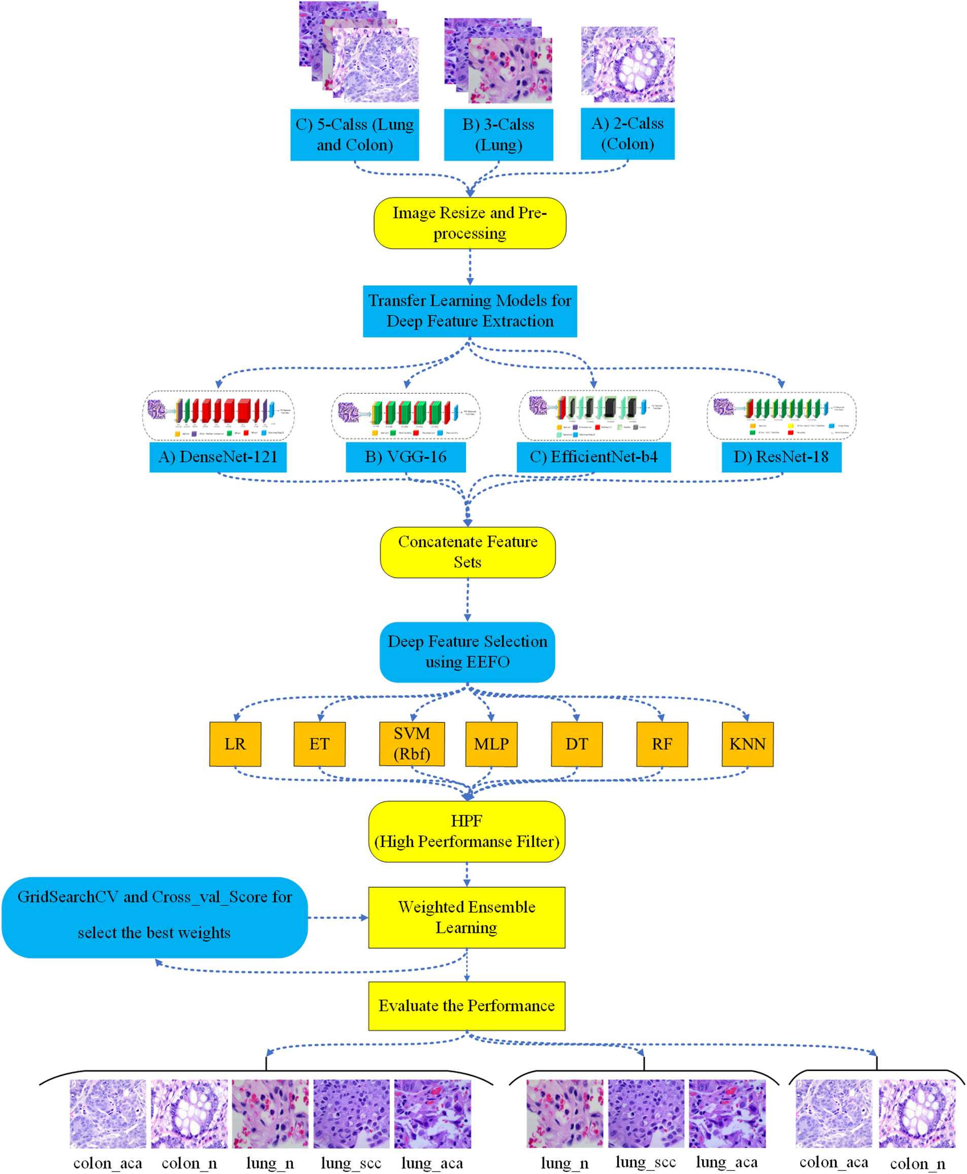
Figure 1: Proposed model for lung and colon cancer detection

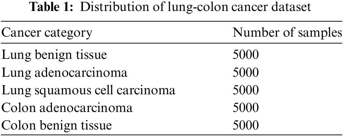
3.1 Description of LC25000 Dataset

The LC25000 dataset, collected by Andrew Burkovsky and his team at James Tampa Hospital in Florida, USA [42], comprises 25,000 images, segregated into two categories of colon cancer and three categories of lung cancer. The distribution of images across these five categories is uniform, indicating that the dataset is balanced with each category containing 5000 images. The categories include colon_aca, represented by images of adenocarcinoma; colon_n, represented by images of benign colon tissues; lung_aca, represented by images of lung adenocarcinoma; lung_scc, represented by images of squamous cell lung cancer; and lung_n, represented by images of benign lung tissue. The lung-colon cancer dataset’s distribution is displayed in Table 1.

3.2 Data Preprocessing

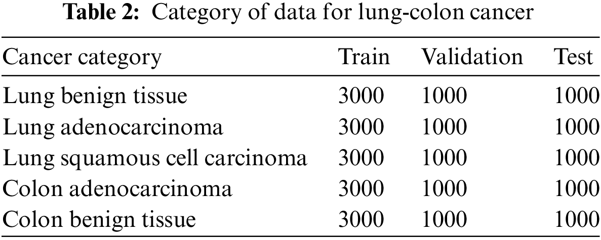
In this step, the original histopathological images of dimensions 768 × 768 are resized to a resolution of 224 × 224. Subsequently, these images are randomly partitioned into training images (60%), validation images (20%), and test images (20%). The training and validation images are utilized to train the classifiers and fine-tune the controllable parameters of the proposed model. This process encompasses training various ML algorithms, selecting optimal features, applying the HPF filter, and adjusting the weights of the ensemble model. It is crucial to reserve the test images for evaluating the model’s generalizability on independent new unseen data.

The enhancement of the input images, achieved through noise reduction and the optimization of significant features, is crucial for the extraction of pertinent information. This process ensures the images’ compatibility with deep CNN models and ML networks. In the spatial domain, averaging filters are generally used to remove noise. There are different types of noise, and for removing each type of noise, a suitable filter exists that should be selected. In the proposed method, noise removal from images is achieved using the fastNlMeansDenoisingColored algorithm, which is based on the Non-Local Means (NLM) method. Currently, a variety of image enhancement techniques are being utilized. One such approach involves improving the image contrast. A prevalent method for enhancing the contrast of low-quality images is the histogram equalization technique. This technique modifies the gray levels of the image to span the entire possible range. The fundamental concept involves mapping the intensity brightness values via a transfer distribution function.

Histogram equalization enhances the contrast of an image relative to its original state, thereby improving image quality and augmenting the accuracy of subsequent processing. Despite its ability to boost image contrast, the resultant image often exhibits an unnatural enhancement and intensity saturation. While it is effective in delineating borders and edges between distinct objects, it may diminish local details. The data category for colon and lung cancer is displayed in Table 2. Overfitting mainly occurs when the training and test data are the same or when the data lacks diversity. To address overfitting, we ensure complete separation of training, test, and validation data, as shown in Table 2. Furthermore, our dataset is balanced across classes, further reducing the risk of overfitting. This approach helps maintain the model’s generalizability and robustness.

After transforming the scaled image into the RGB space, the fastNlMeansDenoisingColored algorithm, which is grounded in the NLM technique, is employed to eliminate noise present in the color images. The fastNlMeansDenoisingColored algorithm identifies analogous patterns in the vicinity of each pixel by utilizing the information contained within the image and subsequently eliminates noise based on these patterns. When a color image is subjected to noise, the color data of each pixel is influenced by this noise, leading to alterations in both the color and intensity of the respective pixel. The fastNlMeansDenoisingColored algorithm, by computing the weighted average of the color values of adjacent pixels, endeavors to mitigate these alterations and restore the image to its original, noise-free state. The fastNlMeansDenoisingColored algorithm proves particularly effective in eliminating noise in low-quality images, images afflicted with speckle noise and images captured under low-light conditions.

The image undergoes a transformation from the RGB (Red, Green, Blue) color space to the LAB color space, and the L channel is subsequently isolated from the LAB image. Following this, color balancing procedures are executed on the L channel utilizing the equalizeHist function, and the L channel is then amalgamated with the A and B channels of the LAB image procured from the preceding step. The image is then reverted to the RGB color space and normalized. In the next step, the intensity and clarity of the image are adjusted randomly, and automatic contrast adjustment operations are conducted on the image. Afterward, the image is converted into the Tensor format. Preprocessing images not only augments the power of distinction in human visual perception but also bolsters this capability in DL algorithms. Fig. 2 describes the pre-processing steps.

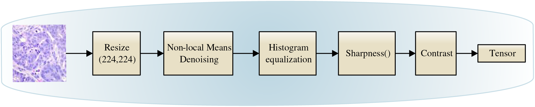
Figure 2: Preprocessing steps

3.3 Features Extraction Using CNNs

The crux of learning lies in the accurate detection of features from the data. Learning models operate on these features to yield the outcome. One method of feature extraction involves the use of DL models, specifically CNNs. In the proposed method, four pre-trained CNNs (VGG16, ResNet18, DenseNet121, and EfficientNet-b4) are employed for 2-Class, 3-Class, and 5-Class tasks. These CNN models extract 4096, 512, 1024, and 1792 features from each image, respectively.

In this study, transfer learning [43] is used to extract features from the input images. Initially, the primary layers of each CNN model are frozen, and the training images are processed through these layers. It allows the model to leverage learned features from extensive pre-training to enhance its ability to extract meaningful features from new images. Thus, the features extracted by these deep layers encapsulate valuable information about the images. These features are subsequently utilized as input for ML algorithms. Applying this transfer learning methodology is anticipated to facilitate the extraction of high-quality features, thereby enhancing the performance of ML algorithms. This approach leverages the power of pre-trained models to extract meaningful features, which can significantly improve the effectiveness of subsequent ML tasks.

3.4 Feature Selection

The purpose of a feature selection algorithm is to reduce the dimension of the dataset in terms of the extracted features. This process can be conceptualized as an optimization problem that aims to maximize the predictive power of the model with the minimum number of features. Considering the NP (Non-deterministic Polynomial)-hardness of this problem, it is beneficial to use metaheuristic algorithms that prove an effective solution approach for the NP-hard problems.

This paper presents a metaheuristic-driven method for reducing dimensionality in the original feature set using EEFO [44], a bio-inspired algorithm inspired by electric eels’ intelligent group search behaviors. The algorithm balances exploration and exploitation, with an energy factor managing global to local search transitions. A feasible solution within the EEFO algorithm (i.e., an electric eel) to solve the feature selection problem in this paper is encoded as a binary string of length N, where N is the total number of original features. Fig. 3 represents a feasible solution, wherein “1” means the selection and “0” means the absence of the corresponding feature within the solution.

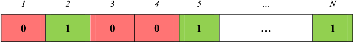
Figure 3: Represent of a feasible solution in the EEFO algorithm

At every iteration of the EEFO algorithm, each generated solution is evaluated using a fitness function. The proposed fitness function, as defined in Eq. (1), combines the accuracy of the model with the effect of the EEFO approach on feature selection and strikes a balance between model accuracy and reducing the complexity of feature selection for more efficient and effective performance.

FitnessFunction(i)=w×Acci+(1−w)×(1−∑FiN)(1)

where w represents the importance of accuracy in the fitness function, Acci is the calculated accuracy of the i-th solution, and Fi is the number of selected features by the i-th solution.

In the proposed feature selection algorithm, as shown in Fig. 4, EEFO starts with an initial population of candidate feature sets and refines and updates feature subsets using an evolutionary optimization technique. The energy coefficient plays a key role in EEFO and governs the selection of search behaviors. If the energy coefficient exceeds 1, the algorithm performs an exploratory behavior, and conversely, when the energy coefficient is less than or equal to 1, a behavior (either resting, hunting or migration) is randomly selected with equal probability and carried out for exploitation.

Figure 4: Overall flowchart of the EEFO algorithm

3.4.1 Interaction

Interaction in EEFO is based on the behavior of electric eels, which form a large electrified circle by coordinating swimming and waving movements. Each electric eel in EEFO serves as a candidate solution, with each step selecting the optimal solution. Eels communicate using their peers’ position data and interact with regional information in the search space. One can formulate this operational method as follows:

A=n1×B(2)

n1∼N(0,1)(3)

B=[b1,b2,…bk,…,bd](4)

b(k)={1ifk==g{l}0else(5)

g=randperm(Dim)(6)

l=1,…,[(MaxIt−ItMaxIt×rand1×(Dim−2)+2)](7)

where MaxIt is the maximum number of iterations in the EEFO algorithm, A is a random vector that determines the direction and magnitude of the eel’s random movement in the search space, B is a binary vector that specifies which dimension of the search space should be considered for this random movement, and g generates a random number equal to the number of original features. Furthermore, the interactive behavior can be defined as follows:

{{wi(It+1)=xj(It)+A×(x¯(It)−xi(It))P1>0.5wi(It+1)=xj(It)+A×(xr(It)−xi(It))P1≤0.5fit(xj(It))<fit(xi(It)){wi(It+1)=xi(It)+A×(x¯(It)−xj(It))P2>0.5wi(It+1)=xi(It)+A×(xr(It)−xj(It))P2≤0.5fit(xj(It))≥fit(xi(It))(8)

x¯(It)=1n∑i=1nxi(It)(9)

xr=Low+r×(Up−Low)(10)

where P1 and P2 are random numbers within (0,1), n stands for the population size, rand1 is a random number in the range (0, 1), and r is a random vector within the same range. Furthermore, the function fit(xi(It)) calculates the fitness of the i-th electric eel candidate’s position, while xj is the position of an eel that is randomly selected from the current population, with the condition that j≠i. Moreover, Low and Up denote the lower and upper boundaries, respectively. According to Eq. (8), the interactive behavior enables electric eels to navigate toward various positions in the search space, significantly aiding EEFO in thoroughly exploring the entire search space.

3.4.2 Resting

In the EEFO algorithm, a rest zone is defined before the electric fish’s rest phase. This region in the search space normalizes each dimension of the fish position vector to a random value between 0 and 1. The search space randomly selects and predicts one dimension. This value is considered to be the center of the rest zone. Each dimension of the eel’s position vector receives a normal random value in this rest region. The purpose of this resting area is to help the eels search better and increase the algorithm’s efficiency. Based on these descriptions, we can characterize the resting place as follows:

{X|X−Z(It)≤α0×|Z(It)−xprey(It)|}(11)

α0=2⋅(e−eItMaxIt)(12)

Z(It)=Low+z(It)×(Up−Low)(13)

Z(It)=xrand(n)rand(Dim)(It−Lowrand(Dim))Uprand(Dim)−Lowrand(Dim)(14)

where xprey denotes the position vector of the best solution found so far, while α0 is the initial scale of the resting area. The expression α0×|Z(It)−xprey(It)| defines the range of the resting area. The term xrand(n)rand(Dim) refers to the random position of an individual, randomly selected from the current population. Lastly, Z is a normalized number. Consequently, the resting state of an electric eel, prior to executing resting behavior within its resting area, can be determined as follows:

Ri(It+1)=Z(It)+α×|Z(It)−xprey(It)|(15)

α=α0×sin⁡(2π×rand2)(16)

where α denotes the scale of the resting area, and rand2 is a random number selected from the interval (0, 1). The scale α is designed such that as the iterations continue, the range of the resting area diminishes. This results in an increased focus on exploitation.

Once the resting area is determined, the electric eels navigate toward it for rest. In other words, an electric eel updates its position to align with its resting state within the defined resting area. The resting behavior can be modeled as follows:

wi(It+1)=Ri(It+1)+n2×(Ri(It+1)round(rand)×xi(It))(17)

n2∼N(0,1)(18)

3.4.3 Hunting

The electric eels swim collectively until they finally form a large circle around their prey. Through their electric organ discharge, the eels communicate and work cooperatively. A rise in interaction reduces the size of the circle into some sort of hunting zone. The prey moves about erratically threat-driven to escape from the hunting zone.

The hunting zone is a dynamic area where electric eels collectively besiege and move the prey from deeper to shallower waters. In the hunting zone, the prey experiences sudden and successive disturbances, causing it to move erratically and unpredictably in different positions in the hunting space. The hunting zone can be defined as follows:

{X|X−xprey(It)|≤β0×|x¯(It)−xprey(It)|}(19)

β0=2×(e−eItMaxIt)(20)

where β0 is the initial scale of the hunting area. From Eq. (19), an electric eel focuses on the prey whose hunting range is determined by the expression β0×|x¯(It)−xprey(It)|. Therefore, a new gray position, relative to its previous position in the hunting area, can be calculated as follows:

Hprey(It+1)=xprey(It)+β×|x¯(It)−xprey(It)|(21)

β=β0×sin⁡(2π×rand3)(22)

where β is the scale of the hunting area and rand3 is a random number within (0, 1). The scale parameter β is defined such that the range of the hunting area decreases over time. This enhances the algorithm’s ability to exploit the search space.

An electric eel initiates a hunting zone by quickly locating the prey’s new position, coiling around it, and generating a high-voltage electric field in the surrounding area. This behavior, characterized by EEFO, updates the eel’s position to align with the prey’s new location. The electric eel uses a coiling motion to initiate physical contact with its prey, allowing it to maintain close proximity and generate a high-voltage electric field, immobilizing the prey for effective hunting. The coiling behavior of electric eels during hunting can be described as follows:

wi(It+1)=Hprey(It+1)+η×(Hprey(It+1)−round(rand)×xi(It))(23)

where η is the coiling coefficient, which can be defined as follows:

η=erand4(1−It)MaxIt×cos⁡(2π×rand4)(24)

where rand4 is a random number within (0, 1).

3.4.4 Migration

When the electric eels find prey, they tend to migrate from the resting area to the hunting area. The following equation is used to mathematically model the migration behavior of the electric eels:

wi(It+1)=−rand5×Ri(It+1)+rand6×Hr(It+1)−L×(Hr(It+1)−xi(It))(25)

Hr(It+1)=xprey(It)+β×|x¯(It)−xprey(It)|(26)

where Hr can be interpreted as any position within the hunting area, while rand6 and rand5 are random numbers within the range (0, 1). The expression Hr(It+1)−xi(It) signifies that the electric eels are migrating towards the hunting area. L represents the Levy flight function, which is incorporated into the exploitation phase of EEFO to avoid becoming ensnared in local optima. L can be determined as follows:

L=0.01×|u⋅σ|v|1C|(27)

u,v∼N(0,1)(28)

σ=(Γ(1+C)×sin⁡(πC2)Γ(1+C2)×C×2C−12)1C(29)

where Γ is the standard gamma function, and C = 1.5.

The electric eel can detect the location of its prey through a minor electrical discharge, enabling it to adjust its position as needed. If the electric eel senses the proximity of the prey during the foraging process, it advances toward the prospective position. Conversely, if the prey is not within close range, the electric eels maintain their existing position. The position of the electric eels is updated according to the following equation:

xi(It+1)={xi(It)fit(xi(It))≤fit(wi(It+1))wi(It+1)fit(xi(It))>fit(wi(It+1))(30)

3.4.5 Transition from Exploration to Exploitation

In EEFO, search behaviors are governed by an energy agent. This agent can adeptly manage the transition between exploration and exploitation phases, thereby enhancing the optimization performance of the algorithm. The energy coefficient value of the electric eel is utilized to choose between exploration and exploitation. The energy coefficient E in the EEFO algorithm is defined as follows:

E(It)=4×sin⁡(1−ItMaxIt)×ln1rand7(31)

As rand7 generates a random number between 0 and 1, Eq. (31) illustrates that E diminishes as the iterations progress. When E > 1, the electric eels display reciprocal behavior and conduct a global search across the entire variable space, thereby initiating exploration. On the other hand, when E < 1, electric eels are inclined to conduct a local search within a promising sub-region. This is achieved through migration, resting, or hunting behaviors, which leads to exploitation. During the initial half of the iterations, exploration is the predominant behavior, while the latter half is characterized by a higher likelihood of exploitation. Based on [44], the likelihood of engaging in either exploration or exploitation during the whole optimization process is roughly 50%. It contributes to maintaining an equilibrium between exploration and exploitation.

3.5 Ensemble Learning Model

The features derived from the preceding stage serve as inputs for seven ML algorithms: RF, LR, DT, SVM-RBF, ET, MLP, and KNN. These algorithms execute the learning process, and the method’s performance is assessed based on their outputs. After training the different ML models, the HPF filter identifies the top three most efficient ML algorithms for the learning process. To achieve this purpose, the performance of various ML algorithms is assessed and ranked according to their accuracy on the validation data set, and accordingly, the three algorithms with the highest accuracy are chosen for the ensemble learning model. Adopting this approach ensures that the ensemble learning model incorporates the most efficient ML algorithms, thereby enhancing the precision of the predictions. After selecting the top three ML algorithms, they are employed during the ensemble learning process to optimize the compatibility and accuracy of the predictions. Eventually, this approach makes the most use of the strengths of different ML algorithms, leading to improved overall efficiency in the ensemble learning model.

In the proposed ensemble learning model, we use the weighted average method to calculate the final output, according to Eq. (32). It is a simple ensemble learning technique in which predictions from multiple models are combined by computing a weighted average [45]. In this method, the prediction of each model is multiplied by a specific weight to obtain the final prediction. By carefully adjusting the weights between 0 and 1, it is possible to give more importance to the prediction of specific models in the final output. By assigning higher weights to models that perform well on specific tasks or datasets, we can create a set that is stronger and more accurate than any other model. However, the main challenge is determining the optimal weights for each model, which can be a time-consuming and computationally expensive process.

Ensemblew=∑i=1nwi×MLi∑i=1nwi(32)

where wi denotes the weight associated with each MLi, and n is the number of different ML algorithms in the ensemble model.

In the proposed weighted average technique, GRidSearchCV and Cross_val_Score are used to select the best weights. GridSearchCV searches among these combinations of parameters to find the best weights that optimize the performance of the ensemble model. cross_val_score is a function that can be used to evaluate the performance of each model in the set using cross-validation. We use cross_val_score to evaluate the accuracy of each model and assign weights based on their performance. More specifically, the weight of each selected ML model is proportional to its normalized accuracy level on the validation dataset. Algorithm 1 displays the pseudo-code of the proposed weighted average ensemble learning model.

4  Research Finding

In this section, we assessed our final model using the LC25000 dataset and our suggested approach utilizing measures such as accuracy, precision, recall, and F1-score. Here is a list of all the acquired findings, together with the necessary graphics. During the experiment, we evaluated the EEFO with the following parameters: 50 eels and a maximum of 100 repetitions. The experiments were carried out on a device equipped with Windows 10 Pro, an Intel® Core™ i7-9700 processor operating at a frequency of 3.00 GHz, 8 cores, a 512 GB SSD (Solid State Drive), a 1 TB hard disk, and 16 GB of RAM (Random Access Memory).

4.1 Evaluation Metrics

In the following, we will examine the criteria of accuracy, precision, recall, and F1-score. In the proposed classification method, one of the following cases will occur based on a comparison between the system’s predicted label and the actual label for each test instance:

•   True Positive (TP) represents the condition where the algorithm correctly identifies individuals with lung and colon cancer.

•   False Negative (FN): a state in which the algorithm mistakenly identifies individuals with lung cancer and colon as healthy.

•   False Positive (FP) occurs when some individuals are healthy, but the algorithm incorrectly diagnoses them with cancer.

•   True Negative (TN) is a state in which individuals are healthy and the algorithm correctly recognizes this.

Accuracy is the main measure of performance, denoting the proportion of correctly predicted samples to the overall number of predictions, which can be calculated as Eq. (33). Precision can be defined as a quantification of the predicted positive observations. It is derived from the proportion of accurately predicted positive instances to the overall number of positive predictions, and is computed as Eq. (34). Recall is a measure of the proportion of positive observations that were accurately predicted. According to Eq. (35), it is calculated as the ratio of accurately anticipated positives to total positive observations. F1-score can be defined as the mathematical average of the precision and recall values that are derived from a specific classification model. The F1-score can be determined as Eq. (36). Specificity quantifies the ability of a model or a diagnostic test to correctly identify true negative instances, which can be calculated as Eq. (37). Finally, Negative Predictive Value (NPV) measures the ability of a test or model to accurately identify negative instances, which is computed as Eq. (38).

Accuracy=TP+TNTP+FP+TN+FN(33)

Precision=TPTP+FP(34)

Recall=TPFN+TP(35)

F1−score=2×Precision×recallPrecision+recall(36)

Specificity=TNTN+FP(37)

NPV=TNTN+FN(38)

4.2 Performance Evaluation

4.2.1 Evaluation of Deep CNN Models

The results of the different CNNs using MLP at the last layer are reported in Table 3. According to the obtained results, DenseNet121 demonstrated superior performance compared to ResNet18, VGG16, and Efficientnet-b4, in all classification tasks. In addition, DenseNet121 consistently outperformed other models in all classification tests with minimal fluctuations, as seen by its higher F1-score, which assesses both accuracy and recall.

4.2.2 Evaluation of ML Models

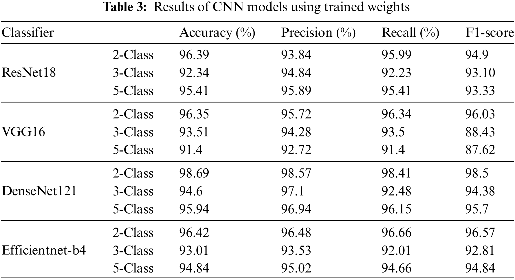
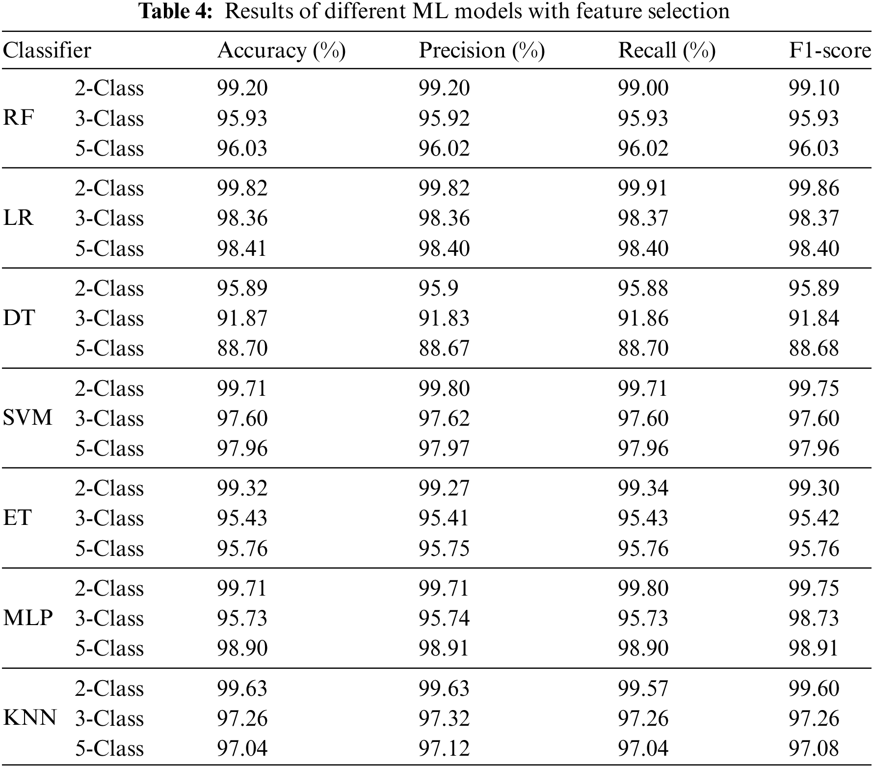
Table 4 shows that all ML models have good accuracy, precision, recall, and F1-score values, suggesting robust categorization. The FR, LR, and SVM classifiers surpass other classification tasks in accuracy, precision, recall, and F1-score, while DT, ET, MLP, and KNN classifiers also perform well, with accuracy ratings of 88.70% to 99.71% across classification tests. Although their accuracy ratings are somewhat lower than RF, LR, and SVM, these models have good precision, recall, and F1-score values, making them suitable for many classification applications.

4.2.3 Evaluation of Feature Selection Algorithm

Fig. 5 demonstrates the convergence curve in 2-Class, 3-Class, and 5-Class scenarios. In the following illustrations, the upper graph typically portrays the number of algorithm iterations at each time point on the horizontal axis, while the vertical axis represents the fitness level. Likewise, the lower graph usually displays the number of iterations of the algorithm at each point in time on the horizontal axis, while the vertical axis displays the number of features selected. Therefore, in our graphical representations, we can see a very gradual and progressive increase in the value of the fitness as the performance of the algorithm progresses towards an optimum point or close to it. Consequently, our approach successfully attains convergence, signifying the algorithm’s achievement of the optimal solution. In fact, this graph shows the number of features that are selected in each iteration. The total number of features is 7424, and each time in each iteration, a number of these features is selected.

Figure 5: Convergence graph of EEFO for (a) 2-Class, (b) 3-Class, and (c) 5-Class scenarios

4.2.4 Evaluation of Ensemble Learning Model

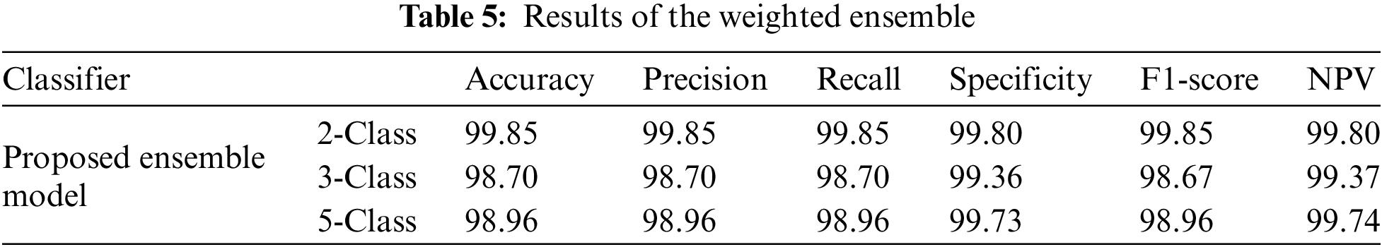
Table 5 demonstrates that the ensemble model outperforms alternative classification models, obtaining outstanding results with accuracy, precision, recall, specificity, F1-score, and NPV, surpassing 99.8% for the 2-Class classification. It continuously exceeds 98.5% in the 3-Class and 5-Class scenarios. The model’s elevated specificity values underscore its dependability in forecasting negative outcomes across diverse categories.

Figs. 6–8 display the Receiver Operating Characteristic (ROC) and confusion matrix for the different scenarios. Fig. 6a outstands the ROC of the different ML algorithms, and Fig. 6b illustrates the confusion matrix of the ensemble model for the 2-Class scenario. Fig. 7a shows the superior performance of the classification algorithms we implemented. As can be seen, we have obtained the highest AUC in the 3-Class scenario. Fig. 7b provides the confusion matrix of the ensemble model for the 3-Class scenario. Fig. 8a illustrates the remarkable efficacy of the classification algorithms we have implemented. As can be discerned, we have attained the utmost AUC in the 5-Class scenario. This outcome resulted in an increase in the TPR (True Positive Rate) and a decrease in the FPR (False Positive Rate), indicating a significant improvement in the proportion of precisely detected positive cases in contrast to real negative instances.

Figure 6: ROC curve and confusion matrix of the proposed model for 2-Class scenario

Figure 7: ROC curve and confusion matrix of the proposed model for 3-Class scenario

Figure 8: ROC curve and confusion matrix of the proposed model for 5-Class scenario

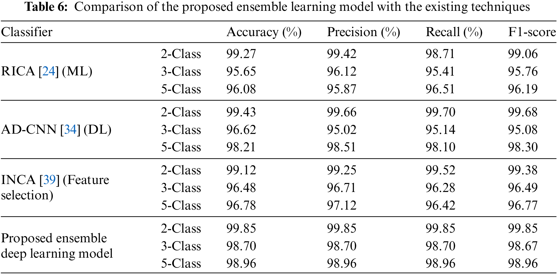
4.2.5 Comparison with Existing Techniques

The comparative analysis of the proposed ensemble learning model with existing techniques is presented in Table 6. Specifically, we have implemented an ML technique known as RICA [24], a DL technique called AD-CNN [34], and a feature selection algorithm termed INCA [39]. To ensure a fair comparison, all techniques were applied to the same lung/colon datasets under identical conditions. The results, as shown in Table 6, clearly illustrate the superiority of the proposed ensemble learning model over all the compared techniques.

5  Conclusion

This study emphasizes the crucial importance of image processing and deep learning in the prompt detection of lung and colon malignancies, leading to early treatment start and enhanced chances of survival. The framework utilizes ensemble deep learning and metaheuristic techniques to accurately predict colon or lung cancer from histopathology pictures with a high level of precision. The work not only emphasizes the need for data pretreatment but also performs noise reduction and contrast enhancement to get precise and pertinent characteristics. Utilizing machine and deep learning algorithms and metaheuristic approaches enhances the performance of the classification model, resulting in exceptional accuracy. Additional comparable approaches were incorporated into the weighted ensemble, and the suggested model demonstrated improved performance in comparison to the others. The results confirm that the proposed model significantly improves the accuracy of diagnosing lung and colon cancers, leading to substantial improvements in patient outcomes and medical treatment options.

The proposed ensemble learning model reduces overfitting through multiple mechanisms. By combining various ML algorithms, it balances the bias-variance tradeoff, improving generalization to unseen data. Averaging predictions from multiple DL and ML models minimizes individual errors, and the diversity of base learners cancels out specific mistakes, leading to more robust and accurate lung/colon cancer classification.

Despite the mentioned advantages, our proposed model has some limitations. One limitation is the lack of external datasets in the model’s analysis, which may not fully capture its performance across diverse real-world scenarios. Future research should aim to expand the model’s applicability by testing it on a broader range of datasets and exploring advanced techniques to enhance both its robustness and transparency. Moreover, aggregation of the multiple CNN and ML models lacks interpretability, making it challenging to understand how the model arrives at its conclusion and the logical basis for its outputs, which poses a challenge in applications requiring transparency and accountability. To address this limitation, we intend to incorporate Explainable AI (XAI) methods in future works.

Acknowledgement: The authors are grateful to editor and reviewers for their valuable comments.

Funding Statement: The authors received no specific funding for this study.

Author Contributions: The authors confirm contribution to the paper as follows: study conception and design: Pouyan Razmjouei, Elaheh Moharamkhani, Mohamad Hasanvand, Maryam Daneshfar, Mohammad Shokouhifar; data collection: Pouyan Razmjouei, Elaheh Moharamkhani, Mohamad Hasanvand, Maryam Daneshfar,; analysis and interpretation of results: Pouyan Razmjouei, Elaheh Moharamkhani, Mohamad Hasanvand, Maryam Daneshfar, Mohammad Shokouhifar; draft manuscript preparation: Pouyan Razmjouei, Elaheh Moharamkhani, Mohamad Hasanvand, Maryam Daneshfar, Mohammad Shokouhifar; revised manuscript preparation: Pouyan Razmjouei, Elaheh Moharamkhani, Maryam Daneshfar, Mohammad Shokouhifar. All authors reviewed the results and approved the final version of the manuscript.

Availability of Data and Materials: The authors confirm that the data supporting the findings of this study are available within the article. The original dataset can be found at: https://www.kaggle.com/datasets/andrewmvd/lung-and-colon-cancer-histopathological-images (accessed on 16 December 2019).

Ethics Approval: Not applicable.

Conflicts of Interest: The authors declare that they have no conflicts of interest to report regarding the present study.

References

1. B. S. A. Bhattacharya, S. Chattopadhyay, and R. Sarkar, “Deep feature selection using adaptive β-Hill Climbing aided whale optimization algorithm for lung and colon cancer detection,” Biomed. Signal Process. Control, vol. 83, no. 6, 2023, Art. no. 104692. doi: 10.1016/j.bspc.2023.104692. [Google Scholar] [CrossRef]

2. N. Kumar, M. Sharma, V. P. Singh, C. Madan, and S. Mehandia, “An empirical study of handcrafted and dense feature extraction techniques for lung and colon cancer classification from histopathological images,” Biomed. Signal Process. Control, vol. 75, no. 1, 2022, Art. no. 103596. doi: 10.1016/j.bspc.2022.103596. [Google Scholar] [CrossRef]

3. N. Maleki and S. T. A. Niaki, “An intelligent algorithm for lung cancer diagnosis using extracted features from Computerized Tomography images,” Healthc. Anal., vol. 3, no. 1, 2023, Art. no. 100150. doi: 10.1016/j.health.2023.100150. [Google Scholar] [CrossRef]

4. B. C. Bade and C. S. D. Cruz, “Lung cancer 2020: Epidemiology, etiology, and prevention,” Clin. Chest Med., vol. 41, no. 1, pp. 1–24, 2020. doi: 10.1016/j.ccm.2019.10.001. [Google Scholar] [PubMed] [CrossRef]

5. C. R. MacRosty and M. P. Rivera, “Lung cancer in women: A modern epidemic,” Clin. Chest Med., vol. 41, no. 1, pp. 53–65, 2020. doi: 10.1016/j.ccm.2019.10.005. [Google Scholar] [PubMed] [CrossRef]

6. B. A. Brock, H. Mir, E. L. Flenaugh, G. Oprea-Ilies, R. Singh and S. Singh, “Social and biological determinants in lung cancer disparity,” Cancers, vol. 16, no. 3, 2024, Art. no. 612. doi: 10.3390/cancers16030612. [Google Scholar] [PubMed] [CrossRef]

7. M. N. Mikhail Lette et al., “Toward improved outcomes for patients with lung cancer globally: The essential role of radiology and nuclear medicine,” JCO Glob. Oncol., vol. 8, 2022, Art. no. e2100100. doi: 10.1200/GO.21.0010. [Google Scholar] [CrossRef]

8. F. Zhu et al., “The value of magnetic resonance imaging in assessing immediate efficacy after microwave ablation of lung malignancies,” J. Thorac. Imaging, vol. 10, 2024, Art. no. 1097. doi: 10.1097/RTI.0000000000000797. [Google Scholar] [PubMed] [CrossRef]

9. M. Li et al., “Research on the auxiliary classification and diagnosis of lung cancer subtypes based on histopathological images,” IEEE Access, vol. 9, pp. 53687–53707, 2021. doi: 10.1109/ACCESS.2021.3071057. [Google Scholar] [CrossRef]

10. Y. Jing et al., “A comprehensive survey of intestine histopathological image analysis using machine vision approaches,” Comput. Biol. Med., vol. 165, no. 3, 2023, Art. no. 107388. doi: 10.1016/j.compbiomed.2023.107388. [Google Scholar] [PubMed] [CrossRef]

11. R. Luo and T. Bocklitz, “A systematic study of transfer learning for colorectal cancer detection,” Inform. Med. Unlocked, vol. 40, 2023, Art. no. 101292. doi: 10.1016/j.imu.2023.101292. [Google Scholar] [CrossRef]

12. K. Lafata, M. Corradetti, J. Gao, C. Jacobs, J. Weng and Y. Chang, “Radiogenomic analysis of locally advanced lung cancer based on CT imaging and intratreatment changes in cell-free DNA,” Radiol.: Imaging Cancer, vol. 3, no. 4, 2021, Art. no. e200157. doi: 10.1148/rycan.2021200157. [Google Scholar] [PubMed] [CrossRef]

13. M. F. Mridha et al., “A comprehensive survey on the progress, process, and challenges of lung cancer detection and classification,” J. Healthc. Eng., vol. 2022, no. 1, pp. 5905230, 2022. doi: 10.1155/2022/5905230. [Google Scholar] [PubMed] [CrossRef]

14. M. Arun Kumar, P. Gopika Ram, P. Suseendhar, and R. Sangeetha, “An efficient cancer detection using machine learning algorithm,” Nat. Volatiles Essent. Oils, vol. 8, no. 4, pp. 6416–6425, 2021. [Google Scholar]

15. M. Masud, N. Sikder, A. -A. Nahid, A. K. Bairagi, and M. A. AlZain, “A machine learning approach to diagnosing lung and colon cancer using a deep learning-based classification framework,” Sensors, vol. 21, no. 3, 2021, Art. no. 748. doi: 10.3390/s21030748. [Google Scholar] [PubMed] [CrossRef]

16. C. de Margerie-Mellon and G. Chassagnon, “Artificial intelligence: A critical review of applications for lung nodule and lung cancer,” Diagn. Interven. Imaging, vol. 104, no. 1, pp. 11–17, 2023. doi: 10.1016/j.diii.2022.11.007. [Google Scholar] [PubMed] [CrossRef]

17. I. Chhillar and A. Singh, “A feature engineering-based machine learning technique to detect and classify lung and colon cancer from histopathological images,” Med. Biol. Eng. Comput., vol. 62, no. 3, pp. 913–924, 2024. doi: 10.1007/s11517-023-02984-y. [Google Scholar] [PubMed] [CrossRef]

18. M. Nishio, K. Nakane, and Y. Tanaka, “Application of the homology method for quantification of low-attenuation lung region inpatients with and without COPD,” Int. J. Chron. Obstruct. Pulmon. Dis., vol. 11, pp. 2125–2137, 2016. doi: 10.2147/COPD.S110504. [Google Scholar] [PubMed] [CrossRef]

19. M. A. Talukder, M. M. Islam, M. A. Uddin, A. Akhter, K. F. Hasan and M. A. Moni, “Machine learning-based lung and colon cancer detection using deep feature extraction and ensemble learning,” Expert. Syst. Appl., vol. 205, 2022, Art. no. 117695. doi: 10.1016/j.eswa.2022.117695. [Google Scholar] [CrossRef]

20. J. Fan, J. Lee, and Y. Lee, “A transfer learning architecture based on a support vector machine for histopathology image classification,” Appl. Sci., vol. 11, no. 14, 2021, Art. no. 6380. doi: 10.3390/app11146380. [Google Scholar] [CrossRef]

21. A. Hage Chehade, N. Abdallah, J. -M. Marion, M. Oueidat, and P. Chauvet, “Lung and colon cancer classification using medical imaging: A feature engineering approach,” Phys. Eng. Sci. Med., vol. 45, no. 3, pp. 729–746, 2022. doi: 10.1007/s13246-022-01139-x. [Google Scholar] [PubMed] [CrossRef]

22. Y. Su et al., “Colon cancer diagnosis and staging classification based on machine learning and bioinformatics analysis,” Comput. Biol. Med., vol. 145, no. 3, 2022, Art. no. 105409. doi: 10.1016/j.compbiomed.2022.105409. [Google Scholar] [PubMed] [CrossRef]

23. N. Maleki, Y. Zeinali, and S. T. A. Niaki, “A k-NN method for lung cancer prognosis with the use of a genetic algorithm for feature selection,” Expert. Syst. Appl., vol. 164, no. 5, 2021, Art. no. 113981. doi: 10.1016/j.eswa.2020.113981. [Google Scholar] [CrossRef]

24. L. Hussain, M. S. Almaraashi, W. Aziz, N. Habib, and S. -U. -R. Saif Abbasi, “Machine learning-based lungs cancer detection using reconstruction independent component analysis and sparse filter features,” Wave. Random Complex, vol. 34, no. 1, pp. 226–251, 2024. doi: 10.1080/17455030.2021.1905912. [Google Scholar] [CrossRef]

25. E. Kayikcioglu, A. H. Onder, B. Bacak, and T. A. Serel, “Machine learning for predicting colon cancer recurrence,” Surg. Oncol., vol. 54, no. 3, 2024, Art. no. 102079. doi: 10.1016/j.suronc.2024.102079. [Google Scholar] [PubMed] [CrossRef]

26. D. Kumar, A. Wong, and D. A. Clausi, “Lung nodule classification using deep features in CT images,” in 2015 12th Conf. Comput. Robot Vis., Halifax, NS, Canada, IEEE, Jun. 3–5 2015, pp. 133–138. doi: 10.1109/CRV.2015.25. [Google Scholar] [CrossRef]

27. A. Teramoto, T. Tsukamoto, Y. Kiriyama, and H. Fujita, “Automated classification of lung cancer types from cytological images using deep convolutional neural networks,” Biomed. Res. Int., vol. 2017, no. 1, pp. 1–6, 2017. doi: 10.1155/2017/4067832. [Google Scholar] [PubMed] [CrossRef]

28. S. Trajanovski et al., “Towards radiologist-level cancer risk assessment in CT lung screening using deep learning,” Comput. Med. Imaging Graph, vol. 90, no. 9, 2021, Art. no. 101883. doi: 10.1016/j.compmedimag.2021.101883. [Google Scholar] [PubMed] [CrossRef]

29. X. Liu, F. Hou, H. Qin, and A. Hao, “Multi-view multi-scale CNNs for lung nodule type classification from CT images,” Pattern Recognit., vol. 77, no. 2, pp. 262–275, 2018. doi: 10.1016/j.patcog.2017.12.022. [Google Scholar] [CrossRef]

30. W. Shen et al., “Multi-crop convolutional neural networks for lung nodule malignancy suspiciousness classification,” Pattern Recognit., vol. 61, no. 4, pp. 663–673, 2017. doi: 10.1016/j.patcog.2016.05.029. [Google Scholar] [CrossRef]

31. H. C. Reis and V. Turk, “Transfer learning approach and nucleus segmentation with medclnet colon cancer database,” J. Digit. Imaging, vol. 36, no. 1, pp. 306–325, 2023. doi: 10.1007/s10278-022-00701-z. [Google Scholar] [PubMed] [CrossRef]

32. N. Ibrahim, N. K. C. Pratiwi, M. A. Pramudito, and F. F. Taliningsih, “Non-complex CNN models for colorectal cancer (CRC) classification based on histological images,” in Proc. 1st Int. Conf. Electron. Biomed. Eng. Health Inform., Surabaya, Indonesia, Springer, 2021, pp. 509–516. doi: 10.1007/978-981-33-6926-9_44. [Google Scholar] [CrossRef]

33. M. Toğaçar, “Disease type detection in lung and colon cancer images using the complement approach of inefficient sets,” Comput. Biol. Med., vol. 137, 2021, Art. no. 104827. doi: 10.1016/j.compbiomed.2021.104827. [Google Scholar] [PubMed] [CrossRef]

34. K. Laxmikant, A. Arthi, V. Vinodhini, B. Natarajan, R. Bhuvaneswari and P. Selvam, “Deep convolutional neural networks for early-stage detection and prognostication of lung and colon cancer,” in 2024 Int. Conf. Int. Circuits Commun. Syst. (ICICACS), IEEE, 2024, pp. 1–6. doi: 10.1109/ICICACS60521.2024.10499027. [Google Scholar] [CrossRef]

35. G. Kumar and H. Alqahtani, “Deep learning-based cancer detection-recent developments, trend and challenges,” Comput. Model. Eng. Sci., vol. 130, no. 3, 2022, pp. 1271–1307. doi: 10.32604/cmes.2022.018418. [Google Scholar] [CrossRef]

36. M. Toğaçar, B. Ergen, and Z. Cömert, “Detection of lung cancer on chest CT images using minimum redundancy maximum relevance feature selection method with convolutional neural networks,” Biocybern. Biomed. Eng., vol. 40, no. 1, pp. 23–39, 2020. doi: 10.1016/j.bbe.2019.11.004. [Google Scholar] [CrossRef]

37. S. Shanthi and N. Rajkumar, “Lung cancer prediction using stochastic diffusion search (SDS) based feature selection and machine learning methods,” Neural Process. Lett., vol. 53, no. 4, pp. 2617–2630, 2021. doi: 10.1007/s11063-020-10192-0. [Google Scholar] [CrossRef]

38. S. P. Khadilkar, “Colon cancer detection using hybrid features and genetically optimized neural network classifier,” Int. J. Image Graph, vol. 22, no. 2, pp. 2250024, 2022. doi: 10.1142/S0219467822500243. [Google Scholar] [CrossRef]

39. J. Rasheed and R. M. Shubair, “Screening lung diseases using cascaded feature generation and selection strategies,” Healthcare, vol. 10, no. 7, pp. 1313, 2022. doi: 10.3390/healthcare10071313. [Google Scholar] [PubMed] [CrossRef]

40. M. G. Lanjewar, K. G. Panchbhai, and P. Charanarur, “Lung cancer detection from CT scans using modified DenseNet with feature selection methods and ML classifiers,” Expert. Syst. Appl., vol. 224, no. 8, pp. 119961, 2023. doi: 10.1016/j.eswa.2023.119961. [Google Scholar] [CrossRef]

41. S. Sucharita, B. Sahu, T. Swarnkar, and S. K. Meher, “Classification of cancer microarray data using a two-step feature selection framework with moth-flame optimization and extreme learning machine,” Multimed. Tools Appl., vol. 83, no. 7, pp. 21319–21346, 2024. doi: 10.1007/s11042-023-16353-2. [Google Scholar] [CrossRef]

42. A. A. Borkowski, M. M. Bui, L. B. Thomas, C. P. Wilson, L. A. DeLand and S. M. Mastorides, “Lung and colon cancer histopathological image dataset (LC25000),” arXiv preprint arXiv:1912.12142, 2019. [Google Scholar]

43. S. Alsubai, “Transfer learning based approach for lung and colon cancer detection using local binary pattern features and explainable artificial intelligence (AI) techniques,” PeerJ. Comput. Sci., vol. 10, no. 6, pp. e1996, 2024. doi: 10.7717/peerj-cs.1996. [Google Scholar] [PubMed] [CrossRef]

44. W. Zhao et al., “Electric eel foraging optimization: A new bio-inspired optimizer for engineering applications,” Expert Syst. Appl., vol. 238, no. 1, pp. 122200, 2024. doi: 10.1016/j.eswa.2023.122200. [Google Scholar] [CrossRef]

45. S. R. Quasar, R. Sharma, A. Mittal, M. Sharma, D. Agarwal and I. de La Torre Díez, “Ensemble methods for computed tomography scan images to improve lung cancer detection and classification,” Multimed. Tools Appl., vol. 83, no. 17, pp. 52867–52897, 2024. doi: 10.1007/s11042-023-17616-8. [Google Scholar] [CrossRef]