A Complex Fuzzy LSTM Network for Temporal-Related Forecasting Problems

1  Introduction

Time-stamped data arises in many areas of real-life applications such as weather, engineering, finance, technology, economics, etc. Various techniques in statistics and machine learning are applied to analyze time-related data or time series data in different domains, including forecasting [1–4], classification [5,6], anomaly detection [7,8], decision making [9,10] and clustering [11–13]. Time series forecasting is an attractive field of research among them. The most frequent issue in this discipline is forecasting data values based on their historical values. In solving the time-stamped, time-series data, many studies are concerned with the influence and relevant factors, and numerous approaches have been proposed in recent decades.

In literature, several different traditional approaches have been used for the time series forecasting problem. Statistical analysis models such as multi-linear regression are well-known, and among the others Integrated Moving Average (ARIMA) method is commonly used to predict the trend of data variables [14–16]. This model is used regularly to forecast time series that are trend stationary, and it is not ideal for non-stationary or weak stationary data. Besides statistical methods, various machine learning (ML) techniques are also used to predict time series problems [17–19]. The statistical methods for forecasting problems often rely on several strict assumptions, such as stationarity, that are not always satisfied in practice. The property of time series is often nonlinear and complex, making it difficult for these methods to capture the actual dynamics. Therefore, some sophisticated ML models have been introduced to address this challenge, but they are also difficult to train and interpret. As a result, no single way can guarantee to build a reliable and robust time-series forecasting model.

Recently, the deep-learning technique was considered as a game-changing method in various challenging prediction problems, including time series forecasting [20–22]. This technique is appropriate to deal with the nature of time series, such as noisy, chaotic, and complex features. Among deep-learning techniques, the long short-term memory (LSTM) is a remarkable framework with time-series data [20]. This is because LSTMs can process and remember elements in time series data and predict dependencies between data efficiently. Instead of remembering historical and immutable information, the LSTM model can determine the context to predict multivariate time series data. Beside LSTM, other studies of deep learning (DL) models using combination strategy that integrates attention based Spatial-Temporal with original DL algorithms to handle time-stamped data, such as Attention based Spatial-Temporal Graph Convolutional Networks (ASTGCN) [23], or attention-based spatial-temporal graph neural networks (ASTGNN) [24]. Each approach has different advantages and disadvantages. Focus on fusing deep learning techniques with fuzzy theory, LSTM would be better to extend with complex fuzzy sets thanks to its natures and simplicity, and therefore in the scope of this study LSTM is a focus point.

In literature, variant models of LSTM were developed for different time series prediction problems. Bandara et al. [25] proposed LSTM-multiseasonal-Net (LSTM-MSNet) that improved the prediction performance by extracting multiple seasonal patterns. Huang et al. [2] proposed a wind speed estimating model due to the combination of LSTM and genetic algorithm (GA). Furthermore, Abbassimehr et al. [26] offered a technique for predicting time series data, that is, a hybrid model combined two deep learning ways: LSTM and multi-head attention. To combine fuzzy theory with the LSTM model, Tran et al. [27] developed an LSTM-based model named multivariate fuzzy LSTM (MF-LSTM) for cloud proactive auto scaling systems that combine different techniques. The researchers used fuzzification techniques to reduce the fluctuation in the input data, and they also used a variable selection method based on the correlation metrics to select a suitable input. In the main phase, they used an LSTM network to predict tasks on multivariate time series data. a prediction model created by Safari et al. [28] that combines LSTM with Interval Type-2 Fuzzy, this model named DIT2FLSTM, was utilized during casting the COVID-19 incidence. The suggested DIT2FLSTM model makes it possible to predict challenging real-world issues like the COVID-19 pandemic by combining the fuzzification technique and LSTM. Langeroudi et al. [29] also proposed a fuzzy LSTM architecture to solve the high-order vagueness. This study proved the potential of fuzzy LSTM in predicting time-series problems. The authors evaluated their approach on several real-world data sets, including the Mackey-Glass (MG), the Sunspot, and the English Premier League datasets. Experiments showed that Deep Fuzzy LSTM could perform top on all these data sets.

Existing studies show that the combination of LSTM and fuzzy theory would generate better prediction performance on time-series data. However, real-life time series data has changed so fast, and nowadays it is often complex and diverse, and that time series data is commonly cyclical and uncertain also. This fact creates a new challenge that traditional models can only handle part of it, which leads to inaccurate predictions and poor performance in many cases. A few studies have been conducted to address this time–cycle issue.

As is widely known, the idea of fuzzy sets (FS) and it extension are a mathematical instrument that can represent uncertainty and vagueness in data [9]. However, traditional fuzzy sets cannot indicate incomplete awareness of data or its alterations at a particular time. This limitation may be problematic when presenting complicated data sets where confusion and unpredictability exist and modify in different periods. To overcome this restriction, Ramot et al. [30] presented an idea of complex fuzzy sets (CFS) as an expansion of traditional FSs. CFSs allow for the representation of partial ignorance and changes in data over time. This makes them a more powerful tool for dealing with uncertainty and vagueness in complex data sets. The distinguishing features of CFSs are complex-valued membership functions containing amplitude and phase elements. Wavelike properties can be represented by CFSs that FSs cannot.

The theory of CFS has led to the development of new models for prediction problems and forecasting time-related datasets in real life, such as Selvachandran et al. [31,32] proposed Mamdani Complex Fuzzy Inference System (CFIS) model. Utilizing CFS, a complex neuro-fuzzy autoregressive integrated moving average presented by Li et al. [33] for predicting the time-series problem. The introduced method combines a modification of the complex neuro-fuzzy system (CNFS) and the ARIMA model to form a new prediction model named CNFS-ARIMA. The CNFS-ARIMA model addressed the nonlinear relationship between output thanks to the characteristics of CFS and ARIMA.

In the way that combines CFS and deep learning models, Yazdanbakhsh et al.’s investigations [34,35] introduced several CFS and neuro-fuzzy combinations. A Fast Adaptive Neuro-CFIS (FANCFIS), a variant of the Adaptive Neuro-CFIS (ANCFIS), was created for quick training. They examined and demonstrated how well the suggested algorithms performed on univariate and multivariate problems. An adaptive spatial CFIS was presented by Giang et al. [36] to identify variations in the data of remote-sensing cloud photos. In comparison to the current most advanced models, the model outperformed them in both terms of speed as well as precision.

In general, combining deep learning models and fuzzy theories could result in better time series prediction models [13]. Because of their advantage, the LSTM model and CFS theory are of interest in creating a new model for temporal-related forecasting, as shown by the theories and techniques mentioned above. This is what motivates us to complete this study that use CFS to represent cyclical input data in a good shape, and this type of data will be processed efficiently in the new design LSTM network. Following are some of the critical contributions made within the context of this work:

(1) Developed a general model of complex fuzzy LSTM for predicting issues involving time theoretically.

(2) Proposed a unique CFLSTM architecture that uses a complex fuzzy LSTM unit to account for the effects of the cycle-time factor on time-series information.

(3) Proved the advantage of the proposed CFLSTM model by comparing its performance with the previously latest developments models based on CFS and other related, including LSTM [37], Fuzzy LSTM [26], ANCFIS [34], on real-world and UCI datasets: an actual monitoring data set of precipitation index in Vietnam, daily temperature index in Melbourne-Australia, and Seoul bike sharing demand from UCI.

The remaining contents are separated into the following sections: Section 2 of the proposal includes background information. The complex fuzzy LSTM model in temporal related forecasting problems is explained explicitly in Section 3. The proposal’s empirical findings and the related forecasting models are evaluated and contrasted in Section 4. The finalizing Section 5 of the paper includes the summary and discussion.

2  Preliminaries

2.1 Complex Fuzzy Set

In 2002, as an expansion of FS theory and fuzzy logic, Ramot et al. [30] presented the definition of CFSs. The CFSs are promising for problems whose meaning changes over time because the “phase” of CFS can represent a changing context, such as a temporal, time-cycle or seasonal factor.

A complex fuzzy membership function μA(x) that has as its range the complex unit circle defines a CFS as follows:

μM(x)=pM(x)ejωM(x),j=−1(1)

where PM(x) is the amplitude and ωM(x) the phase of the CFS, PM(x)∈[0,1] and ωM(x)∈[0,2π].

2.2 Complex Fuzzy Membership Function

A mathematical tool known as a complex fuzzy membership function (CFMF) can transform a crisp input into a fuzzy output in complex fuzzy spaces. Sinusoidal and Gaussian membership functions are two of the most common types of CFM functions.

Sinusoidal membership functions: First introduced by Chen et al. in [38], sinusoidal CFMF over the unit disc codomain is defined as:

rA(θ)=dsin⁡ (a θ+b)+c;θ=x;ω(x)=θ(2)

where the amplitude and the phase of the CFMF are determined by r(θ) and ω(x); The frequency, phase shift, shifts the wave vertically, and the sine wave’s amplitude is altered by the settings a, b, c, d, respectively. The coordinates of μA(θ)=z=x+iy are calculated by the following equations:

x=rcos⁡(θ);y=rsin⁡(θ)(3)

The amplitude of a complex fuzzy membership function must be between 0 and 1. This means that the parameters need to meet the requirements listed below: |d|+|c|≤1 and 0≤d≤c≤1.

Gaussian membership functions: There are four ways to define Gaussian membership functions in complex fuzzy spaces for a unit squared or a unit disc codomain. These four forms were proposed in [39,40].

(1)   The first version is determined in the unit square codomain:

G1(x,m,σ)=Re(G1(x,m,σ))+j Im(G1(x,m,σ))(4)

where Re(.) and Im(.) are, respectively, the real and imaginary factors in the CFMF.

Re(G1(x,m,σ))=e[−0.5(x−mσ)2](5)

Im(G1(x,m,σ))=−e[−0.5(x−mσ)2]×(x−mσ)(6)

(2)   In the unit disc codomain, the second variant is defined:

G2(x.m,σ,λ)=rs(x,m,σ)ejωs(x,m,σ,λ)(7)

where rs and ωs are the complex fuzzy grade’s amplitude and phase, respectively.

rs(x,m,σ)=e[−0.5(x−mσ)2](8)

ωs(x,m,σ,λ)=−e[−0.5(x−mσ)2]×(x−mσ)×λ(9)

Hence, the parameters x∈U as above, m,σ,λ represent the mean, spread, and phase frequency factors in CFS. The phase frequency factor is a parameter that can be adjusted to improve the fit of the membership function to the data.

(3) The Gaussian CFMF is presented as G3(x)=μ(x)=A(x)ejP(x) in the third format suggested in [41], where the amplitude and phase are determined as follows:

A(x)=e(−(x−cAaP)P);P(x)=2πe(−(x−cAaP)P)(10)

(4) The following is the definition of a Gaussian CFMF for the real and imaginary parts of a CFS, which is the fourth form of the Hata et al. proposal [42] for a Gaussian CFMF:

μAR(xr)=e[−(xr−cr)2wr];μAI(xi)=e[−(xi−ci)2wi](11)

where the Gaussian function’s center and width are represented by cr, wr for the real-valued component xr and ci, wi for the imaginary component xi, respectively.

In complex fuzzy set theory, the four Gaussian shape membership functions differ primarily in their parameters, which affect their shape and characteristics. The differences in these parameters allow each Gaussian shape membership function to model different aspects of uncertainty or fuzziness in data. In applications, the researcher has to analyze the data to determine the most suitable membership function.

2.3 The LSTM Model

Among deep-learning techniques, the LSTM architecture [37] is used widely for identifying and predicting issues on time series data. As an advanced improvement on the recurrent neural network (RNN), LSTM was developed to cope with a serious shortcoming in the back-propagating training process, that is the vanishing gradient problem in the RNN. LSTM has the advantage of dealing with long-term dependencies in modeling time-related problems, and therefore, it can improve the quality of time series forecasting problems.

The LSTM contains one or more LSTM units similar to RNN memory cells’ structure to store information over long periods. The detailed design of each unit is represented in Fig. 1. Each unit has three nonlinear gates regulating data flow: the forget gate ft, input gate it, and output gate ot.

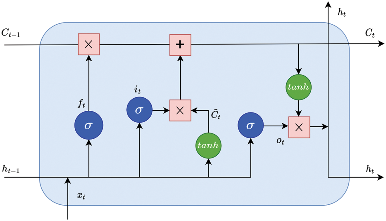
Figure 1: The structure of an LSTM unit

These gates take on different roles in the learning process and can improve training results. In particular, the forget gate ft chooses to erase unnecessary information from the previous state, the output gate ot specifies how the LSTM unit will respond, and the input gate it controls the method for adding new input data.

The correlation throughout the data in the sequence of inputs is captured by the unit. Fig. 1 illustrates detail each unit in the LSTM.

In an LSTM unit, a chain of calculations is performed and lets the LSTM network learn long-term. The calculations of ht and ct at the tth step of the learning process are presented below. Where Ui and Wi are matrices present input and recurrent weights; bi is the bias; σ is a sigmoid activation function, and C~t is the candidate activation.

With an input sequence data x=(x1,x2,…,xt−1,xt) the hidden (output) state h=(h1,h2,…,ht−1,ht) and the unit state c=(c1,c2,…,ct−1,ct). The first input value x1 is used by the first LSTM unit to generate the first hidden state h1 and the first updated unit state c1. And then, at time step t, input value xt and hidden state ht−1 are used by LSTM unit to calculate hidden state ht and the updated unit state ct.

The forget gate is a critical component of LSTMs that decides what information to keep and discard. It removes irrelevant information from the unit’s internal state, allowing LSTM to obtain long-term dependencies. The forget gate ft for a certain time step t can be calculated as follows:

ft=σ(Wf,xxt+Wf,hht−1+bf)(12)

where σ∈[0,1] is the sigmoid function, Wf,x is the forget weight matrix, Wf,h is the forget-hidden weight matrix, and bf is the bias. The input gate it is a control gate that determines whether the information is updated or supplemented to the memory unit. It is calculated using a sigmoid function at time t, as shown as below:

it=σ(Wi,xxt+Wi,hht−1+bi)(13)

where Wi,x and Wi,h are the weight matrix, and the input gate bias bi, respectively.

Then, the value of updating unit state ct at time step t is determined using the value of forget gate ft and the value of input gate it. In which ft controls the amount of information retained or discarded from the unit state ct−1 at time t − 1, the input controls the information inputs at the current time. The candidate value c~t−1 represents new potential information that needs to be added to the internal state of the memory unit. The values Wc~,x, and Wc~,h correspond to the weight matrix and the bias vector of the updated unit state. The value of c~t−1 is defined as follows:

c~t=tan⁡h(Wc~,xxt+Wc~,hht−1+bc~)(14)

After that, the new memory unit state ct is calculated based on the previous memory unit state and the Hadamard (∘) element-wise product, as follows:

ct=ft∘ct−1+it∘c~t(15)

Finally, the output gate ot and the hidden state ht to the next time step are defined as follows:

ot=σ(Wo,xxt+Wo,hht−1+bo)

ht=ot∘tan⁡h(ct)(16)

3  Proposed Complex Fuzzy LSTM Model for Temporal-Related Forecasting Problems

This section of the paper proposes the use of a complex fuzzy LSTM model for temporal-related forecasting problems, this includes some components: complex fuzzy LSTM for temporal-related forecasting issues, components of complex fuzzy LSTM unit, and a complex fuzzy LSTM network architecture that takes care of the effect of cycle time in the model.

3.1 Time-Series Forecasting Problem

In this proposal, we are concerned with the problems of time series forecasting. Formally, given a series of time-stamped values X={x1,x2,…,xT} where xT∈Rn, n is the variable dimension, our objective is to forecast a number of future signals in a rolling method. We assume that {x1,x2,…,xT} are available in order to forecast xT+δ, where δ is the desired horizon forward of the present timestamp. Similarly, we suppose that X={x1,x2,…,xT+1} are available in order to predict the value of the next timestamp, xT+δ+1. Hence, the input matrix of the time series estimating issue is as XT={x1,x2,…,xT}∈Rx×T at timestamp T. The prediction horizon is typically determined by the particular needs of the application, such as those for weather indices like precipitation, temperature, etc.; or the horizon of interest for traffic usage typically hours, while normal seconds or minutes forecast will be useful for stock market data.

In forecasting with time series data, good handling of time-cycle variables will bring higher forecasting efficiency in many cases. A time-cyclical variable is a variable whose change is influenced by the time cycle, and is repetitive within a certain period of time. This type of data differs from other trend of change by time, such as time-decay element, and therefore proper prediction models have to be designed in the way to consider the temporal nature and characteristics of data like time-cycle.

3.2 Proposed Complex Fuzzy LSTM Model

This section presents a complex fuzzy LSTM model with complex fuzzy input data related to time cycle factors. The complex fuzzy LSTM network (CFLSTM) is a deep learning framework that handles complex fuzzy data pertaining to time cycle elements and long-term and short-term movements. In the context of the proposed model, a time cyclical variable is well presented by a suitable complex fuzzy number formation. The Formula (1) in Section 2.1 addresses how the time cycle element is presented in phase of complex fuzzy. And then, this element is processed in gates of fuzzy LSTM by new proposed operations introduced in next section. In general, a brief description of the CFLSTM net architecture is shown in Fig. 2. And in the sections that follow, each component of the CFLSTM net will be discussed in detail.

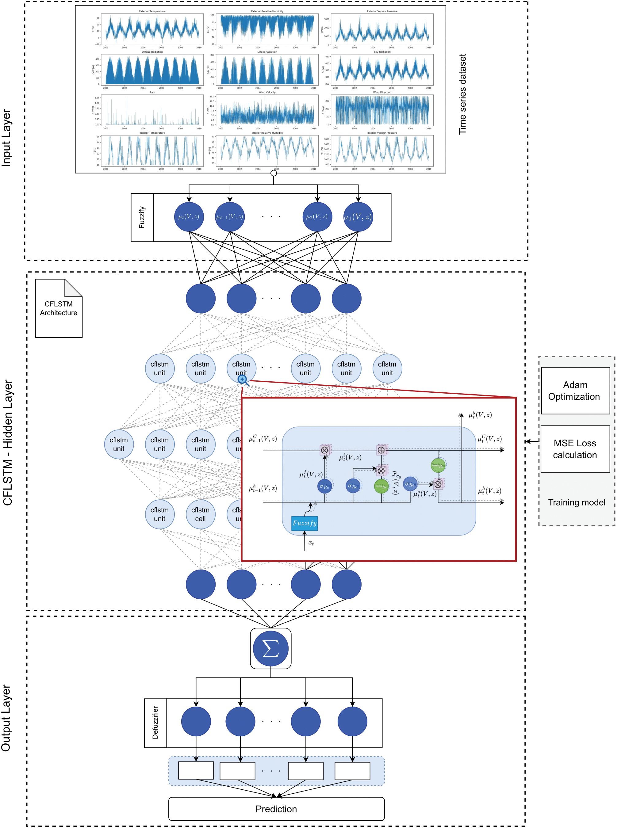
Figure 2: Proposed CFLSTM architecture

The input, hidden, and output layers are three basic components of the CFLSTM network. Below is an explanation of each component’s specifics.

Input layer: This layer is responsible for preprocessing the input data set, which includes processing, structuring, and dividing it for model learning and testing. Assume that at time t, the input vector is processed with a time delay p represented by vector {xt−p,…,xt−2,xt−1}. Next, the vector is then fuzzified using the fuzzy functions as in Section 2.2.

CFLSTM hidden layer and training model: Building the LSTM network architecture and training the model using the training data are the responsibilities of the hidden layer. In Sections 3.3, 3.4 we introduce the basic CFLSTM hidden layer in the network architecture, in which one node of hidden layer employs a CFLSTM unit. Section 3.3 presents a proposal of a unique CFLSTM unit architecture that extends the classical LSTM unit to process complex fuzzy input data, and to account for the effects of cycle time on time-series information. The detail of the CFLSTM unit includes active function and operations of gates is presented in the same section.

The input to this hidden layer is a set of complex fuzzy value vectors, and the loss function utilized during model learning is the MSE function. This study trains the model settings using the Adam optimization approach. Meanwhile, the complex fuzzy LSTM network’s details are being learned using the backpropagation through time (BPTT) algorithm.

Output layer: The proposed LSTM’s output layer defuzzes the hidden layer output from the hidden layer in order to anticipate the data. Either complicated defuzzification routines or a linear layer can be used to execute the defuzzification process. If a linear layer is utilized, the hidden layer’s complex values’ real and imaginary values are aggregated together to generate a real value. The final predicted true value result is produced by processing the inverse data with the earlier encoders.

3.3 CFLSTM Unit

As mentioned above, the hidden layer in the CFLSTM architecture includes CFLSTM units, and the detail of the proposed CFLSTM unit is represented in Fig. 3. In this section, the complex fuzzy values of the variables are used in μt(V,z)=μt,Re(V)+jμt,Im(z) form for the next calculations. Where μt,Re(V) and μt,Im(z) represent the real and imaginary parts of complex fuzzy numbers, respectively.

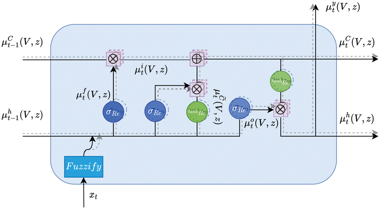
Figure 3: The structure of a complex fuzzy LSTM unit

At the time t, the input value xt is fuzzified to complex fuzzy values using one of the CFMF in Section 2.2.

The gates of the CFLSTM unit are calculated according to the formula as follows:

Input gate at time t is calculated according to the Formula (17):

μt,Rei=σ(Re{μi,xW(V,z)+μi,hW(V,z)μt−1h(V,z)+μib(V,z)});μt,Imi=σ(Im{μi,xW(V,z)+μi,hW(V,z)μt−1h(V,z)+μib(V,z)});(17)

The forget gate is calculated according to the Formula (18)

μt,Ref=σ(Re{μf,xW(V,z)+μf,hW(V,z)μt−1h(V,z)+μfb(V,z)});μt,Imf=σ(Im{μf,xW(V,z)+μf,hW(V,z)μt−1h(V,z)+μfb(V,z)});(18)

The candidate value μtc~ represents new potential information that needs to be added to the internal state of the memory unit. The values μc~,xW, μc~,hW and μc~W are corresponding to weight matrix and the bias vector of the updated unit state. The value of μtc~ is defined as follows:

μt,Rec~=tan⁡h(Re{μc~,xW(V,z)+μc~,hW(V,z)μt−1h(V,z)+μc~b(V,z)});μt,Imc~=tan⁡h(Im{μc~,xW(V,z)+μc~,hW(V,z)μt−1h(V,z)+μfc~(V,z)});(19)

After that, the new memory unit state μtc is calculated based the previous memory unit state and the Hadamard (∘) element-wise product, as follows:

μt,Rec=μt,Ref∘μt−1,Rec+μt,Rei∘μt,Rec~;μt,Imc=μt,Imf∘μt−1,Imc+μt,Imi∘μt,Imc~;(20)

The output gate μto is defined as follows:

μt,Reo=tan⁡h(Re{μo,xW(V,z)μtx(V,z)+μo,hW(V,z)μt−1h(V,z)}+μob(V,z));μt,Imo=tan⁡h(Im{μo,xW(V,z)μtx(V,z)+μo,hW(V,z)μt−1h(V,z)}+μob(V,z));(21)

Finally, the hidden state μth to next time step is defined as follows:

μt,Reh=μt,Reo∘tan⁡h(μt,Rec);μt,Imh=μt,Imo∘tan⁡h(μt,Imc);(22)

where σ and tan⁡h are activation functions of complex numbers. Some activation functions of complex numbers are given in Table 1.

3.4 CFLSTM Architecture Detail

Classical LSTM architectures often do not care about the time period problem in network architecture. In many practical problems, the state of a unit at time kΔt has a strong impact on the forecast results at time t, where k is the number of cycles and Δt is a period of time. Therefore, in this section, we present an architecture that is concerned with the time period of the CFLSTM network. The CFLSTM architecture for the time period is shown in Fig. 4.

Figure 4: CFLSTM architecture with period

A CFLSTM unit at time t takes as input the aggregated unit state and hidden state from previous times, with a period of Δt. The aggregated unit and hidden state are estimated by the formula as follows:

The aggregated unit state with window size Δw at kth period is calculated as shown in the Formula (23).

μk,∑Δw,Rec=1Δw∑∀wi∈ΔwRe{μt−(k∗Δt±wi)c(V,z)};μk,∑Δw,Imc=1Δw∑∀wi∈ΔwIm{μt−(k∗Δt±wi)c(V,z)};(23)

And the aggregated hidden state with window size Δw at kth period is calculated as shown in Formula (24).

μk,∑Δw,Reh=1Δw∑∀wi∈ΔwRe{μt−(k∗Δt±wi)h(V,z)};μk,∑Δw,Imh=1Δw∑∀wi∈ΔwIm{μt−(k∗Δt±wi)h(V,z)};(24)

Then, the previous aggregated unit state by period k is calculated by the Formula (25).

μ∑Δt,Rec=1k∑i=0kσ(μk,∑Δw,Rec);μ∑Δt,Imc=1k∑i=0kσ(μk,∑Δw,Imc);(25)

The previous aggregated hidden state by period k is calculated by the Formula (26).

μ∑Δt,Reh=1k∑i=0kσ(μk,∑Δw,Reh);μ∑Δt,Imh=1k∑i=0kσ(μk,∑Δw,Imh);(26)

The next gates of the CFLSTM unit at time t are calculated by using the previous aggregated unit state μ∑Δtc and aggregated hidden state μ∑Δth by period k and window size Δw as a previous state to compute the gates.

The CFLSTM architecture is an extension of the traditional LSTM architecture. When k=0 and Δw=1, the CFLSTM architecture reverts to the conventional LSTM architecture.

3.5 Time Complexity of a CFLSTM

Briefly, assuming the input size is D, the hidden state size is H, window size Δw, length of the time series is N, and number of CFLSTM cells is M, based on Formulas (17)–(19), the time complexity of each gate in the CFLSTM unit is O (2D.H+2H2+2H) and then single CFLSTM has time complexity O (8H.D+8H2+16H+Δw). Meanwhile, the time complexity of conventional is O (4D.H+4H2+12H). Assume that the training process stops in N number of iterations (number of epochs), its time complexity is N.O (L.M(8H.D+8H2+16H+Δw)), where L is the input time series, and M is the number of CFLSTM cells.

4  Results of Experiments and Application

The experimental comparison of the proposed model is covered in this section, along with datasets, evaluative measurements, and comparison models. Three comparison scenarios are used to show the efficacy and advantages of the proposed model compared to other models: the model developed using a complex fuzzy set (ANCFIS) and the model developed using only machine learning algorithms (LSTM and Fuzzy LSTM).

4.1 Experimental Datasets and Evaluative Metrics

The study used three datasets—one set of precipitation monitoring data observed by month, one set of temperature data observed by day, and one set of standard UCI data about car sharing in Seoul collected hourly—to illustrate the benefits of the proposed model in forecasting time series datasets. The datasets’ specifics are as follows:

(1) The World Bank’s published precipitation dataset. From 1901 through 2021, this data was observed over a 12-month period. Due to their varied geographical locations, the precipitation data from three provinces in Vietnam—Hanoi, Thua Thien-Hue, and Ho Chi Minh—were chosen to evaluate the proposed model’s relationship to meteorological parameters, including time series and cycles. With data on precipitation for three provinces—Ha Noi, Thua Thien Hue, and Ho Chi Minh, and one third of data series are selected to display in Fig. 5 to better present data characteristic in visualization.

Figure 5: The one-third series of the precipitation dataset at Vietnam

(2) Daily minimum temperature in Melbourne, Australia dataset. This dataset contains 3650 observations of the daily min/max temperature in Melbourne, Australia, from 1981–1990, min = 0 and max = 26.3. Fig. 6 shows temperature data for Melbourne, Australia in the first one-third sub-set of original data.

Figure 6: The one-third series of the temperature dataset at Melbourne, Australia

(3) A typical UCI time series database is the demand for bike sharing in Seoul. The dataset provides an hourly rental bicycle count for the Seoul Bike Sharing System. It has 8760 observations spread out throughout 24 h from 01 December to 30 November 2017. The first one-third sub-set of the original dataset for bike sharing in Seoul is shown in Fig. 7. The sub-set is selected to better present data characteristics in visualization.

Figure 7: The one-third series of the Seoul bike sharing demand dataset

Evaluation methods and metrics: The study compares the model that was proposed to LSTM [37], Fuzzy LSTM [29], and ANCFIS [34] on the three metrics of Root Mean Squared Error (RMSE); Mean Absolute Error (MAE) and Symmetric Mean Absolute Percentage Error (SMAPE), which are designed to empirically demonstrate the efficiency of the proposed model:

MAE=∑i=1n|y^i−yi|n;(27)

RMSE=∑i=1n(y^i−yi)2n;(28)

SMAPE=∑i=1n|y^i−yi|(|y^i|+|yi|)/2n;(29)

In this instance, y^i is the value that the model predicts, and yi is the actual value that was seen.

4.2 Experimental Results

Experimental environment: The experimental process was conducted on computers with the following specifications: Intel(R) Core(TM) i9-9900K CPU @ 3.60 GHz; 16 GB RAM; Python language and PyTorch library were used to install and run the experiments.

Experimental process: For each dataset, the data was splitted into training dataset and testing dataset randomly. The proposed model was trained on training set with the parameters presented in Table 2. After building a model, it was used to test on the testing set and report the result. This process is repeated 10 times, and the value of error metrics is average of 10 testing times.

The CFLSTM model’s parameters is setted as follows:

Experimental results: After our test was complete, the following results were obtained: In Fig. 8, which depicts the learning process, the loss function values for each dataset are displayed.

Figure 8: Training process of proposed models for different data series

The Fig. 8 shows that with the learning rate setted at 0.0003 and other parameters presented in Table 2, the models convergence reach after 600 epochs. After epoch 600, the loss values reduce very slowly.

According to the period parameters k = 1, 2, 3, Table 3 and Figs. 9–11 display the results of the predictions made by CFLSTM for each dataset: Precipitation Vietnam, Melbourne Temperature, and Seoul Bike Sharing.

Figure 9: CFLSTM’s results for the precipitation Vietnam dataset

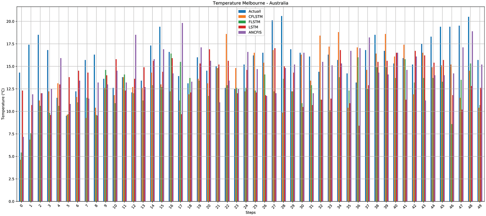
Figure 10: CFLSTM’s results for the Melbourne temperature dataset

Figure 11: CFLSTM’s results for the Seoul bike sharing dataset

The result in Table 3 suggests that the models usually give better results when k>0, and for different data series, the best found k parameter is different. For the dataset of Seoul bike sharing the optimal result reached at k=1, and the optimal result reached at k>1 for other datasets.

Results of algorithm performance metrics were estimated by average values of 10 times running the test. Note that the results depicted in Figs. 9–11 are the best case in all testing times, that present the loss and the trend of prediction performance.

Table 3 shows the MAE and RMSE and SMAPE results on three datasets: Precipitation Vietnam, Melbourne temperature, and Seoul Bike Sharing. As shown in Table 3, the time period factor has a strong impact on the forecast results, with MAE and RMSE gradually decreasing with k = 0, 1, 2, 3, respectively. This is especially pronounced for the Precipitation Vietnam and Melbourne temperature datasets. Therefore, finding this parameter is one of the important tasks when using proposed CFLSTM in applications.

4.3 Comparison and Analysis

By contrasting the outcomes of the proposed model with those of three other models-LSTM [37], Fuzzy LSTM [29], and ANCFIS [34]-the benefits of the suggested CFLSTM model are shown in this section.

Table 4 and Figs. 9–11 show the results of the models’ forecasting using three datasets that are related to the temporal factors. As shown in Table 4, the CFLSTM model using k=1 has significantly lower MAE, RMSE and SMAPE values than the LSTM and Fuzzy LSTM models. Compared with the ANCFIS neural network applying complex fuzzy theory, the proposed model also gives lower MAE, MSE and SMAPE measure results on experimental datasets. This demonstrates that when forecasting data relating to time factors, such as time series and time periods, the suggested CFLSTM model outperforms conventional models like LSTM, Fuzzy LSTM, and ANCFIS.

Besides above advantage, as mentioned above the proposed CFLSTM is more time complexity than the classical LSTM model. This is the trade off for handling time-cycle factor in manner of complex fuzzy set and the extending operations of CFLSTM gates. However, the experiment with datasets above show that this consuming time is till handleable with the hardware configuration mentioned in Section 4.2. In cases of larger data set or real-time forecasting, the model would require high computational resource and it need further experiment to make complete judgement. Furthermore, in practice there is the risk of overfitting in the training process and this effects the accuracy of a designed model on new, unseen data. Users can apply some techniques in the training process to avoid this risk, that includes setting of suitable drop-out rate and batch size.

5  Conclusions

This study combines complex fuzzy theory with LSTM to create a CFLSTM neural network. In the complex fuzzy LSTM neural network, we are interested in the period-time factor in the input data, and use complex fuzzy process to better tackle these factors. The designed model could empower the LSTM architecture in processing the time cycle factors. The proposed model has been experimentally installed and verified through 03 data sets: precipitation monitoring data of three regions of Hanoi, Hue, and Ho Chi Minh City from 1901–2021; daily temperature monitoring data from Melbourne-Australia; and Seoul bike sharing demand data from UCI. The proposed model shows that the prediction error through 2 indicators, MAE and RMSE, is smaller than that of the LSTM, Fuzzy LSTM, and ANCFIS models. The forecast results of the proposed model give quantitative predictive value. Rainfall closely follows the observed real trend for the time period datasets.

Experimental results indicate that the CFLSTM model demonstrates significant potential for forecasting time series data, however it also has higher computational complexity than classical LSTM. Furthermore, additional research is required to thoroughly evaluate the trade-off between improved accuracy and increased consuming time. Consequently, future research efforts will focus on advancing the mathematical operations underlying the CFLSTM operator and identifying efficient computational strategies for handling large datasets.

Acknowledgement: The authors are grateful to all the editors and anonymous reviewers for their comments and suggestions.

Funding Statement: This work was funded by the Research Project: THTETN.05/23-24, Vietnam Academy of Science and Technology.

Author Contributions: Study conception and design: Nguyen Tho Thong, Cu Nguyen Giap, Nguyen Long Giang, Luong Thi Hong Lan; data collection: Luong Thi Hong Lan, Nguyen Van Quyet; analysis and interpretation of results: Nguyen Tho Thong, Cu nguyen Giap, Nguyen Long Giang; draft manuscript preparation: Nguyen Tho Thong, Luong Thi Hong Lan. All authors reviewed the results and approved the final version of the manuscript.

Availability of Data and Materials: The datasets used in this study are openly available from UCI at https://archive.ics.uci.edu/dataset/560/seoul+bike+sharing+demand, accessed on 18 June 2023, and from the corresponding author on reasonable request.

Ethics Approval: Not applicable.

Conflicts of Interest: The authors declare that they have no conflicts of interest to report regarding the present study.

References

1. N. Bacanin et al., “Multivariate energy forecasting via metaheuristic tuned long-short term memory and gated recurrent unit neural networks,” Inf. Sci., vol. 642, 2023, Art. no. 119122. doi: 10.1016/j.ins.2023.119122. [Google Scholar] [CrossRef]

2. C. Huang, H. R. Karimi, P. Mei, D. Yang, and Q. Shi, “Evolving long short-term memory neural network for wind speed forecasting,” Inf. Sci., vol. 632, no. 20, pp. 390–410, 2023. doi: 10.1016/j.ins.2023.03.031. [Google Scholar] [CrossRef]

3. P. Li, H. Gu, L. Yin, and B. Li, “Research on trend prediction of component stock in fuzzy time series based on deep forest,” CAAI Trans. Intell. Technol., vol. 7, no. 4, pp. 617–626, 2022. doi: 10.1049/cit2.12139. [Google Scholar] [CrossRef]

4. D. N. Tuyen et al., “Rainpredrnn: A new approach for precipitation nowcasting with weather radar echo images based on deep learning,” Axioms, vol. 11, no. 3, 2022, Art. no. 107. doi: 10.3390/axioms11030107. [Google Scholar] [CrossRef]

5. F. Karim, S. Majumdar, H. Darabi, and S. Chen, “LSTM fully convolutional networks for time series classification,” IEEE Access, vol. 6, pp. 1662–1669, 2017. doi: 10.1109/ACCESS.2017.2779939. [Google Scholar] [CrossRef]

6. F. Karim, S. Majumdar, H. Darabi, and S. Harford, “Multivariate LSTM-FCNS for time series classification,” Neural Netw., vol. 116, no. 2, pp. 237–245, 2019. doi: 10.1016/j.neunet.2019.04.014. [Google Scholar] [PubMed] [CrossRef]

7. T. Ergen and S. S. Kozat, “Unsupervised anomaly detection with LSTM neural networks,” IEEE Trans. Neural Netw. Learn. Syst., vol. 31, no. 8, pp. 3127–3141, 2019. doi: 10.1109/TNNLS.2019.2935975. [Google Scholar] [PubMed] [CrossRef]

8. B. Lindemann, B. Maschler, N. Sahlab, and M. Weyrich, “A survey on anomaly detection for technical systems using LSTM networks,” Comput. Ind., vol. 131, no. 3, 2021, Art. no. 103498. doi: 10.1016/j.compind.2021.103498. [Google Scholar] [CrossRef]

9. T. Mahmood, Z. Ali, D. Prangchumpol, and T. Panityakul, “Dombi-normalized weighted bonferroni mean operators with novel multiple-valued complex neutrosophic uncertain linguistic sets and their application in decision making,” Comput. Model. Eng. Sci., vol. 130, no. 3, pp. 1587–1623, 2022. doi: 10.32604/cmes.2022.017998. [Google Scholar] [CrossRef]

10. L. T. H. Lan, D. T. T. Hien, N. T. Thong, F. Smarandache, and N. L. Giang, “An anp-topsis model for tourist destination choice problems under temporal neutrosophic environment,” Appl. Soft Omput., vol. 136, no. 7, 2023, Art. no. 110146. doi: 10.1016/j.asoc.2023.110146. [Google Scholar] [CrossRef]

11. S. Aghabozorgi, A. S. Shirkhorshidi, and T. Y. Wah, “Time-series clustering–A decade review,” Inf. Syst., vol. 53, no. 12, pp. 16–38, 2015. doi: 10.1016/j.is.2015.04.007. [Google Scholar] [CrossRef]

12. H. Du, S. Du, and W. Li, “Probabilistic time series forecasting with deep non-linear state space models,” CAAI Trans. Intell. Technol., vol. 8, no. 1, pp. 3–13, 2023. doi: 10.1049/cit2.12085. [Google Scholar] [CrossRef]

13. J. Gu et al., “Research on short-term load forecasting of distribution stations based on the clustering improvement fuzzy time series algorithm,” Comput. Model. Eng. Sci., vol. 136, no. 3, pp. 2221–2236, 2023. doi: 10.32604/cmes.2023.025396. [Google Scholar] [CrossRef]

14. S. Khan and H. Alghulaiakh, “Arima model for accurate time series stocks forecasting,” Int. J. Adv. Comput. Sci. Appl., vol. 11, no. 7. 2020. doi: 10.14569/IJACSA.2020.0110765. [Google Scholar] [CrossRef]

15. S. Siami-Namini and A. S. Namin, “Forecasting economics and financial time series: ARIMA vs. LSTM,” arXiv preprint arXiv:1803.06386, 2018. [Google Scholar]

16. S. Mehrmolaei and M. R. Keyvanpour, “Time series forecasting using improved ARIMA,” in 2016 Artif. Intell. Robot. (IRANOPEN), IEEE, 2016. [Google Scholar]

17. F. Li and C. Wang, “Develop a multi-linear-trend fuzzy information granule based short-term time series forecasting model with k-medoids clustering,” Inf. Sci., vol. 629, no. 4, pp. 358–375, 2023. doi: 10.1016/j.ins.2023.01.122. [Google Scholar] [CrossRef]

18. A. Borovykh, S. Bohte, and C. W. Oosterlee, “Conditional time series forecasting with convolutional neural networks,” arXiv preprint arXiv:1703.04691, 2017. [Google Scholar]

19. M. Castán-Lascorz, P. Jiménez-Herrera, A. Troncoso, and G. Asencio-Cortés, “A new hybrid method for predicting univariate and multivariate time series based on pattern forecasting,” Inf. Sci., vol. 586, no. 4, pp. 611–627, 2022. doi: 10.1016/j.ins.2021.12.001. [Google Scholar] [CrossRef]

20. X. Fan, Y. Wang, and M. Zhang, “Network traffic forecasting model based on long-term intuitionistic fuzzy time series,” Inf. Sci., vol. 506, no. 1, pp. 131–147, 2020. doi: 10.1016/j.ins.2019.08.023. [Google Scholar] [CrossRef]

21. A. Zeroual, F. Harrou, A. Dairi, and Y. Sun, “Deep learning methods for forecasting COVID-19 time-series data: A comparative study,” Chaos, Solit. Fractals, vol. 140, no. 50, 2020, Art. no. 110121. doi: 10.1016/j.chaos.2020.110121. [Google Scholar] [PubMed] [CrossRef]

22. Y. Dong, L. Xiao, J. Wang, and J. Wang, “A time series attention mechanism based model for tourism demand forecasting,” Inf. Sci., vol. 628, no. 3, pp. 269–290, 2023. doi: 10.1016/j.ins.2023.01.095. [Google Scholar] [CrossRef]

23. S. Guo, Y. Lin, N. Feng, C. Song, and H. Wan, “Attention based spatial-temporal graph convolutional networks for traffic flow forecasting,” in Proc. AAAI Conf. Artif. Intell., vol. 33, no. 1, pp. 922–929, 2019. doi: 10.1609/aaai.v33i01.3301922. [Google Scholar] [CrossRef]

24. B. Wang, F. Gao, L. Tong, Q. Zhang, and S. Zhu, “Channel attention-based spatial-temporal graph neural networks for traffic prediction,” Data Technol. App., vol. 58, no. 1, pp. 81–94, 2024. doi: 10.1108/DTA-09-2022-0378. [Google Scholar] [CrossRef]

25. K. Bandara, C. Bergmeir, and H. Hewamalage, “LSTM-MSNet: Leveraging forecasts on sets of related time series with multiple seasonal patterns,” IEEE Trans. Neural Netw. Learn. Syst., vol. 32, no. 4, pp. 1586–1599, 2020. doi: 10.1109/TNNLS.2020.2985720. [Google Scholar] [PubMed] [CrossRef]

26. H. Abbasimehr and R. Paki, “Improving time series forecasting using LSTM and attention models,” J. Ambient Intell. Humaniz. Comput., vol. 13, no. 1, pp. 1–19, 2022. doi: 10.1007/s12652-020-02761-x. [Google Scholar] [CrossRef]

27. N. Tran, T. Nguyen, B. M. Nguyen, and G. Nguyen, “A multivariate fuzzy time series resource forecast model for clouds using LSTM and data correlation analysis,” Procedia Comput. Sci., vol. 126, no. 6, pp. 636–645, 2018. doi: 10.1016/j.procs.2018.07.298. [Google Scholar] [CrossRef]

28. A. Safari, R. Hosseini, and M. Mazinani, “A novel deep interval type-2 fuzzy LSTM (DIT2FLSTM) model applied to COVID-19 pandemic time-series prediction,” J. Biomed. Inform., vol. 123, no. 7, 2021, Art. no. 103920. doi: 10.1016/j.jbi.2021.103920. [Google Scholar] [PubMed] [CrossRef]

29. M. K. Langeroudi, M. R. Yamaghani, and S. Khodaparast, “Fd-LSTM: A fuzzy LSTM model for chaotic time-series prediction,” IEEE Intell. Syst., vol. 37, no. 4, pp. 70–78, 2022. doi: 10.1109/MIS.2022.3179843. [Google Scholar] [CrossRef]

30. D. Ramot, M. Friedman, G. Langholz, and A. Kandel, “Complex fuzzy logic,” IEEE Trans. Fuzzy Syst., vol. 11, no. 4, pp. 450–461, 2003. doi: 10.1109/TFUZZ.2003.814832. [Google Scholar] [CrossRef]

31. G. Selvachandran et al., “A new design of mamdani complex fuzzy inference system for multiattribute decision making problems,” IEEE Trans. Fuzzy Syst., vol. 29, no. 4, pp. 716–730, 2019. doi: 10.1109/TFUZZ.2019.2961350. [Google Scholar] [CrossRef]

32. L. T. H. Lan, T. M. Tuan, T. T. Ngan, N. L. Giang, V. T. N. Ngoc and P. Van Hai, “A new complex fuzzy inference system with fuzzy knowledge graph and extensions in decision making,” IEEE Access, vol. 8, pp. 164899–164921, 2020. doi: 10.1109/ACCESS.2020.3021097. [Google Scholar] [CrossRef]

33. C. Li and T. -W. Chiang, “Complex neurofuzzy ARIMA forecasting new approach using complex fuzzy sets,” IEEE Trans. Fuzzy Syst., vol. 21, no. 3, pp. 567–584, 2012. doi: 10.1109/TFUZZ.2012.2226890. [Google Scholar] [CrossRef]

34. O. Yazdanbakhsh and S. Dick, “Time-series forecasting via complex fuzzy logic,” in Frontiers of Higher Order Fuzzy Sets, 2015, pp. 147–165. [Google Scholar]

35. O. Yazdanbakhsh and S. Dick, “FANCFIS: Fast adaptive neuro-complex fuzzy inference system,” Int. J. Approx. Reason., vol. 105, no. 3, pp. 417–430, 2019. doi: 10.1016/j.ijar.2018.10.018. [Google Scholar] [CrossRef]

36. N. L. Giang, N. Van Luong, L. T. H. Lan, T. M. Tuan, and N. T. Thang, “Adaptive spatial complex fuzzy inference systems with complex fuzzy measures,” IEEE Access, vol. 11, pp. 39333–39350, 2023. doi: 10.1109/ACCESS.2023.3268059. [Google Scholar] [CrossRef]

37. S. Hochreiter and J. Schmidhuber, “Long short-term memory,” Neural Comput., vol. 9, no. 8, pp. 1735–1780, 1997. doi: 10.1162/neco.1997.9.8.1735. [Google Scholar] [PubMed] [CrossRef]

38. Z. Chen, S. Aghakhani, J. Man, and S. Dick, “ANCFIS: A neurofuzzy architecture employing complex fuzzy sets,” IEEE Trans. Fuzzy Syst., vol. 19, no. 2, pp. 305–322, 2010. doi: 10.1109/TFUZZ.2010.2096469. [Google Scholar] [CrossRef]

39. C. Li and T. -W. Chiang, “Complex fuzzy computing to time series prediction multi-swarm PSO learning approach,” in Intell. Inform. Database Syst.: Third Int. Conf., ACI-IDS 2011, Daegu, Republic of Korea, Berlin Heidelberg, Springer, 2011, pp. 242–251. [Google Scholar]

40. C. Li and T. -W. Chiang, “Function approximation with complex neuro-fuzzy system using complex fuzzy sets-a new approach,” New Gener. Comput., vol. 29, no. 3, pp. 261–276, 2011. doi: 10.1007/s00354-011-0302-1. [Google Scholar] [CrossRef]

41. R. Shoorangiz and M. H. Marhaban, “Complex neuro-fuzzy system for function approximation,” Int. J. Appl. Electron. Phys. Robot., vol. 1, no. 2, pp. 5–9, 2013. doi: 10.7575/aiac.ijaepr.v.1n.2p.5. [Google Scholar] [CrossRef]

42. R. Hata and K. Murase, “Generation of fuzzy rules by a complex-valued neuro-fuzzy learning algorithm,” Intell. Inform., vol. 27, no. 1, pp. 533–548, 2015. [Google Scholar]

43. K. Tachibana and K. Otsuka, “Wind prediction performance of complex neural network with ReLU activation function,” in 2018 57th Annu. Conf. Soc. Instrum. Control Eng. Japan (SICE), Nara, Japan, IEEE, 2018, pp. 1029–1034. [Google Scholar]

44. P. Virtue, X. Y. Stella, and M. Lustig, “Better than real: Complex-valued neural nets for MRI fingerprinting,” in 2017 IEEE Int. Conf. Image Process. (ICIP), Beijing, China, IEEE, 2017, pp. 3953–3957. [Google Scholar]

45. T. Kim and T. Adali, “Fully complex backpropagation for constant envelope signal processing,” in Neural Netw. Signal Process. X. Proc. 2000 IEEE Signal Process. Soc. Workshop (Cat. No. 00TH8501), Sydney, NSW, Australia, IEEE, 2000, vol. 1, pp. 231–240. [Google Scholar]

46. R. Savitha, S. Suresh, N. Sundararajan, and P. Saratchandran, “A new learning algorithm with logarithmic performance index for complex-valued neural networks,” Neurocomputing, vol. 72, no. 16–18, pp. 3771–3781, 2009. doi: 10.1016/j.neucom.2009.06.004. [Google Scholar] [CrossRef]

47. N. Guberman, “On complex valued convolutional neural networks,” arXiv preprint arXiv:1602.09046, 2016. [Google Scholar]

48. Y. Özbay, “A new approach to detection of ECG arrhythmias: Complex discrete wavelet transform based complex valued artificial neural network,” J. Med. Syst., vol. 33, no. 6, pp. 435–445, 2009. doi: 10.1007/s10916-008-9205-1. [Google Scholar] [PubMed] [CrossRef]

49. N. Benvenuto and F. Piazza, “On the complex backpropagation algorithm,” IEEE Trans. Signal Process., vol. 40, no. 4, pp. 967–969, 1992. doi: 10.1109/78.127967. [Google Scholar] [CrossRef]

50. D. T. La Corte and Y. M. Zou, “Newton’s method backpropagation for complex-valued holomorphic multilayer perceptrons,” in 2014 Int. Joint Conf. Neural Netw. (IJCNN), Beijing, China, IEEE, 2014, pp. 2854–2861. [Google Scholar]

51. T. Nitta, “Solving the XOR problem and the detection of symmetry using a single complex-valued neuron,” Neural Netw., vol. 16, no. 8, pp. 1101–1105, 2003. doi: 10.1016/S0893-6080(03)00168-0. [Google Scholar] [PubMed] [CrossRef]

52. H. Leung and S. Haykin, “The complex backpropagation algorithm,” IEEE Trans. Signal Process., vol. 39, no. 9, pp. 2101–2104, 1991. doi: 10.1109/78.134446. [Google Scholar] [CrossRef]