Value Function Mechanism in WSNs-Based Mango Plantation Monitoring System

1  Introduction

The plantation sector supports domestic and export needs in Taiwan, one of which is mango plantations. Based on data from the Taiwan Council of Agriculture, mango plantations have increased in the last 5 years both in terms of production and the amount of plantation land. In 2021, the yield of mango plantations in Taiwan will reach 171,662 million metric tons with an agricultural land area of 16,393 hectares. With high levels of mango production in Taiwan, mango is in the top 5 of plantation products exported to several countries, mainly the United States, Japan, Hong Kong, Singapore, and Mainland China. The demand for mango exports needs to be balanced with balanced production results to meet domestic and export needs, especially with the challenges faced, including the shortage of labor, farmer aging, and global competition [1]. One of the efforts made to maintain stability and optimize the production of mango plantations is to monitor the environmental conditions of the mango plantation [2]. Monitoring which is carried out continuously has a positive impact on mango plantations in controlling potential plant diseases, facilitating irrigation arrangements where monitoring can be known through soil moisture, and optimal plant growth through temperature and humidity conditions. However, several problems that occur in efforts to monitor the condition of mango plantations, especially conventional monitoring, are high labor costs, the lack of data analysis processes that provide insights for users, and monitoring carried out was not in real-time conditions. The use of technology can be an alternative in overcoming problems related to monitoring, where several studies have been carried out by combining plantation technology, plantation engineering, and integration with technological devices such as IoT, deep learning, and machine vision [3,4] to support the mango plantation production process. The implementation of IoT technology that integrates a variety of sensors to monitor crops provides many advantages for farmers, both in terms of the precision of the resulting data, validity, ease of implementation, and cost-effectiveness. So that farmers can easily monitor plantation conditions in real-time and remotely. The IoT technology could be adopted in order to maintain, monitor, and control the agricultural system by integrating with AI technology, such as fault detection for Japanese plum [5], greenhouse fig plantation monitoring systems [6], smart irrigation using IoT [7], real-time monitoring for lettuce growth in hydroponics [8]. The IoT technology could also be integrated with wireless sensor networks (WSNs) in the physical layer to obtain real-time data from multiple sensors or devices. This constant influx of information enables better monitoring, automation, and resource management, revolutionizing industries and creating a more interconnected and data-driven system.

To achieve automation in the monitoring plantation system, WSNs technology is employed, integrating nodes to gather input from specific parameters, process this data, and produce output as actuators and real-time data. Belupu et al. [9] developed a WSNs tool as part of monitoring in rural areas to see how the banana plants are growing. WSNs technology is connected to LoRA then the data is stored in the NoSQL database. Benyezza et al. [10] collaborated WSNs with fuzzy logic, where the system can run according to the rules built to control various plant varieties. Meanwhile, Muhammad et al. [11] utilized GPRS-GSM technology in implementing WSNs in porang plantations. This study does not only utilize WSNs technology in plantation monitoring but in combination with deep reinforcement learning (DRL) as part of the system in making a decision or analytical data on the results of reading nodes in the form of real-time conditions. Table 1 shows the results of a comparative analysis of this study with the previous research:

This paper is organized into several sections as follows: Section 2, a literature review, describes the related works and theoretical aspects related to the study. Section 3 presents the materials and methods. Section 4, results and discussions, presents the findings of the experiment and examines the proposed DQN model applied to real data in the mango plantation environment. Section 5 concludes the work.

2  Literature Review

2.1 Related Works

Related work regarding DRL implementation in the monitoring system, among others, was carried out by De Castro et al. [12] in the agriculture sector. They utilized DRL combined with random trees, employing unmanned aerial vehicles (UAVs) for path planning to detect pests in olive trees. The experiment utilizes a scenario with 4 test points, A, B, C, and D, which are distributed across 3 paths: AB, BC, and CD. The test results show that the DRL and random trees combination method shows a run time of 8.2 m/s. Din et al. [13] used multi-agent in DRL implementation which uses the dual deep Q-network (DDQN) method in the field of precision agriculture (PA). The test scenario is through comparison with other algorithms, i.e., uniform coverage (UC), individual Q-learning (IQL), and behavior-based robotics coverage (BBR). The final results indicate that the DDQN achieves higher accuracy, with an 85% coverage area, compared to UC, IQL, and BBR, which average below 80%. Li et al. [14] employed DRL on wheat crop based on mobile edge computing. Agent is designed with a combination of deep Q-network (DQN), with experimental results showing lower energy consumption by 128%. Zhou [15] implemented DRL on agricultural irrigation which aims to control irrigation and save water resources.

The AI-driven techniques could be integrated into WSNs in order to enhance the performance of the monitoring system, as represented in the previous study. AgriTera was invented to estimate the quality and ripeness of fruit by non-invasive accuracy through sub-terahertz wireless signals. Two parameters are employed, including Brix and Dry Matter to estimate fruit ripeness and quality. In the experimental stage, by comparing with the ground truth, AgriTera can estimate Brix and Dry Matter with an outstanding normalized RMSE of 0.55% [16]. Aryai et al. [17] implemented a metaheuristic-driven machine learning routing protocol (MDML-RP) in the monitoring system, which is motivated by integrating machine learning’s real-time capabilities and metaheuristic’s superior route optimization methods. In the simulation experiment, the MDML-MP model has superior performance compared to the existing metaheuristic, heuristic, and protocol of machine learning. Memarian et al. [18] introduced TSFIS-GWO which is the metaheuristic learning model combined with fuzzy heuristic for wireless network reactive routing protocol. This method’s purpose is to take advantage of both fuzzy heuristics’s speed for real-time routing and metaheuristics’ efficacy for offline hyperparameter tuning. The fuzzy inference system is Takagi-Sugeno in conjunction with Gray Wolf optimizer. Experiment results demonstrate that the proposed TSFIS-GWO model is effective in providing real-time solutions to optimize the performance of wireless network protocol.

There are several statistical tools to optimize precision agricultural control including machine learning, data mining, and predictive models. Kocian et al. [19] described that statistical methods could be applied to the system to predict future data. There are several combined statistical techniques and machine learning technologies that could be implemented to enhance the performance of precision farming: low-order statistics, regression, classification method, clustering, artificial neural networks, and Bayesian time-series forecasting. Furthermore, reinforcement learning could provide the system with more intelligence by agent-based decision-making. The system can solve complex problems from the related environment by several parameters. The successful implementation of reinforcement learning can be seen in computer games, energy management, and medical diagnosis systems. This approach can also be applied in agricultural fields to optimally solve complex tasks in dynamic environments. Tao et al. [20] employed a combined imitation learning and reinforcement learning to optimize crop management by controlling nitrogen fertilization and water irrigation. The simulation involves a decision support system for agrotechnology transfer. To maintain a large number of stated variables, the deep Q-network is employed so that it can achieve optimum policies. Experimental simulations in maize crops indicate a profit improvement of more than 45%.

Meanwhile, in the study, DRL is combined with WSNs to build an intelligent mango plantation monitoring system. DRL operates through an agent that uses the state information read by the WSNs from the mango plantation environment to generate an action. This action takes the form of a recommendation, indicating whether the environmental conditions are ‘optimal,’ ‘sub-optimal,’ or ‘not-optimal.’ The state that becomes the basis for the agent in carrying out the action consists of three parameters, including humidity, soil moisture, and temperature. The agent processes the state through a learning model, which in this case employs the Q-network that consists of knowledge in the form of scenarios of environmental conditions in the form of states and actions. The Q-network is composed of a deep neural network (DNN) arrangement that has previously processed data for training. The action produced by the agent then becomes feedback on the model, which is called a reward. So that the agent’s knowledge will continue to enhance along with new data and information from the received state.

2.2 Markov Decision Process (MDP)

The implementation of Markov Decision Process (MDP) mathematical framework is widely used for decision-making in the field of reinforcement learning in dynamic, uncertain, and random environments [21]. Within the MDP there is a terminology agent which has a role as a decision-making entity based on environmental conditions. The agent acts to decide action a based on state s, with the transition from each state represented by reward r. Eq. (1) represents how s, a, r are related in a cycle [22], where si, ai, ri are the initial conditions in a neutral condition. st, at, rt represent immediate returns in one cycle and at the end the agent transitions each episode until it reaches the final condition sterminate.

(si, ai, ri)→(st, at, rt)→(st+1, at+1, rt+1)→…→sterminate(1)

The final target in MDP is to achieve the optimal return in the form of policy π* which is formulated using Eq. (2) which for given state s, argmaxa∈A specifies the action that maximizes Q-value policy which is represented by Qπ∗(s, a) [23].

π∗(s)=argmaxa∈AQπ∗(s, a)(2)

The agent has been given an understanding of the environmental conditions in the form of a state, then determines what action to take and the reward that becomes the basis for producing the next state [24]. The MDP value function can be represented by the Bellman equation as shown by Eq. (3) below:

V(s)=max[a]{sum[s′, r]P(s′, r|s, a)×[r+γ×V(s′)]}(3)

In Eq. (3), V(s) denotes the value of state s, while max[a]{ … } represents the maximum possible action value of a. P(s′, r|s, a) is a sequential probability where the movement from state s to state s′ and there is a reward r when action a is performed. The reward, represented by r, is obtained after action a is performed. The notation of γ denotes a discount factor that functions as a counterweight between the immediate reward and the future reward. Singh et al. [25] described that network devices can be solved with a framework of constrained MDP. Generally, the MDP framework has a set of states and actions that are both finite and discrete. This is because the model must determine the most efficient path within a continuous state and action space [26]. De Giacomo et al. [27] used MDP in the construction of a digital twin in smart manufacturing which is a bridge between the real and virtual worlds in determining models, predicting, optimizing, and understanding related to real assets. MDP aims to produce optimal policies from certain scenarios. The final results indicate that the optimal policy derived from the MDP can select the best service, characterized by low cost and a minimal chance of breaking.

2.3 Deep Reinforcement Learning

Basically, machine learning is divided into two parts: supervised and unsupervised learning. However, in its development, another development emerged from machine learning, i.e., reinforcement learning (RL) [23]. RL has a fundamental difference from supervised learning in that RL works based on specific scenarios to determine the best path based on agent decisions called actions. The agent in RL gets the input parameter in the form of the state of the environment and determines what action to take, by generating a reward as a basis for consideration to produce a new state in the next phase [28]. In RL, MDP is the basis for modeling the environment and how agents interact with the environment to produce actions or decisions [29]. The components contained in RL consist of environment, agent, policy, and reward which are visually represented by Fig. 1.

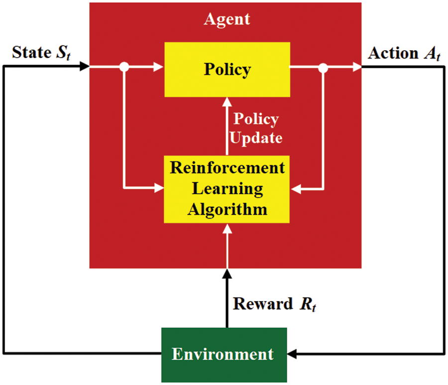
Figure 1: The component of reinforcement learning

In Fig. 1, the agent receives the state St from the environment as the basic parameter for the agent to make decisions. In the decision-making process, there is an RL algorithm that interacts with the policy as an approximator or selector for the best decision that can be made by the agent. The output of the decision is represented in the form of an action At which will later return to the environment to become a cumulative reward during the process of carrying out the task. Learning algorithms update knowledge by continuously updating policies based on conditions from state, action, and reward [30]. Cumulative rewards based on action and state, then multiplied by a discount factor γ as represented in Eq (4):

Rt=rt+γ2rt+2+…+γnrt+n=∑t=0T−1γtrt+1(4)

RL is combined with deep neural networks to become deep reinforcement learning which can handle problems that have high-dimensional and continuous state or action [31]. In DRL, agents employ deep neural networks (DNN) to estimate the policy and value functions as formulated in Eq. (5):

πθ=Pr(a|s,θ)≈π(a|s)(5)

Several studies related to DRL include the work of Elaziz et al. [32], who employed a method combining deep reinforcement learning (DRL) with a variational autoencoder (VAE) for detecting anomalies in the business process. The scenarios contained in the dataset are divided into training data by 80% and test data by 20%. From the results of the model evaluation, the highest accuracy is 92.98%. Hou et al. [33] implemented actor-critic algorithm as a real-time process simulation in DRL to produce the best model. Based on the matrix evaluation, the proposed model is a DRL-based recommender system model (DRR-Max) with the best accuracy. In this research, DRL implementation is combined with deep Q-network (DQN) through a series of scenarios represented in the dataset. Modeling is carried out with variations in initial parameters to produce DQN models with the best accuracy to produce reliable, precise, and valid models.

3  Materials and Methods

3.1 System Architecture

In general, the current system of the plantation monitoring system consists of three layers: the physical layer, the network layer, and the application layer. The physical layer consists of integrating sensor devices with microcontrollers. The sensor reads environmental conditions in the form of soil moisture, temperature and humidity conditions which are then processed by the microcontroller so that they can be represented as the current condition of the plantation environment. The data is then transmitted to the network layer, where in this layer there is a Wi-Fi module as a transmitter with the user via the application layer. In the network layer data can be stored into the cloud platform database or sent directly to the user. While the application layer serves as the top layer where the user can interact directly with the system, it is also important to consider how sensor readings on the physical layer are transmitted in real-time. Fig. 2 illustrates the current system for monitoring plantations.

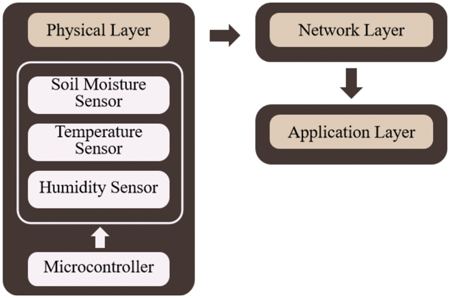
Figure 2: Monitoring plantation current system

The existing system, which refers to the IoT architecture, consists of the physical layer, network layer, and application layer, the improvements and integration have been made to the physical layer and network layer, which are later called the sensor and network layer. In the sensor and network layer, it integrates various sensors, microcontrollers, and Wi-Fi modules into interconnected nodes through a structured network called wireless sensor networks (WSNs). This aims to increase the efficiency of transmitting the results of data readings carried out by sensors on parameters so that they can be accessed quickly by the user. So the architectural context of the concept in this study is integration between the basic architecture of IoT with improvements in part of the physical layer through WSNs. The proposed system architecture in the study is represented by Fig. 3 where there are three layers: (1) sensor and network layer, (2) data analytic layer, and (3) application layer. As the explanation mentioned above, the proposed system has advantages wherein the integration of the physical layer is in the form of WSNs which consist of sensor nodes, microcontrollers, and Wi-Fi modules, which provide optimal speed and data processing. Besides, there is a data analytic layer which is an implementation of DRL. The results of reading data on the sensor and network layer are not only limited to the output of real-time conditions, but also the system can analyze the trend of these conditions so as to provide recommendations for the user to make certain decisions. In terms of features compared to the current system, the proposed system is more complex to produce precise and reliable output. WSNs and DRLs are the main features of data processing in an architecture system where it not only collects some data, but data is stored and analyzed through the data analytic layer.

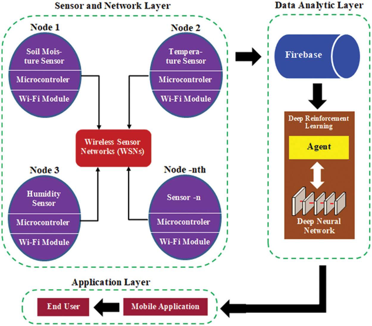
Figure 3: System architecture proposed

At the sensor and network layer, several nodes interact with each other to form a WSN, where each node comprises sensor components, microcontrollers, and Wi-Fi modules. Node 1 is a soil moisture sensor integrated with a microcontroller and Wi-Fi module. Similarly, node 2 and node 3 are the temperature sensor and humidity sensor, respectively. The-nth node indicates that more than 3 nodes can be implemented in the WSNs. The results of reading real-time condition data from the sensor and network layer are then transmitted to the data analytic layer, where Firebase serves as a cloud-based storage system, distributing data in real-time. In the data analytic layer, there is a DRL that processes real-time data before it is distributed to the next layer. Inside the DRL, the agent uses a deep neural network to determine which action to use. In this study, the action performed by the agent is in the form of a binary classification where the agent determines the real-time conditions of the mango plant environment in “optimal”, “sub-optimal” or “not-optimal” conditions. In detail, the mechanism for processing and iterating data in DRL is described in Section 3.3. After the data is processed in the data analytic layer, the next step is to distribute the data to the application layer which uses an Android-based mobile application that can be directly accessed by end users.

The communication process between the sensor and network layer to the Firebase uses the message queuing telemetry transport (MQTT) protocol mechanism. The MQTT protocol works based on machine-to-machine communication where in this case the WSN communicates with Firebase. In the MQTT protocol, there are terms publisher and subscriber where in this case the WSN device acts as a publisher which transmits data through MQTT as a broker to Firebase. MQTT distributes real-time data to Firebase through a cloud gateway and Firebase receives data to redistribute data to mobile applications. In the data network between the mobile application and the Firebase cloud, it uses the hypertext transfer protocol (HTTP) which functions as a real-time data encoder from Firebase to be accessed by the mobile application.

3.2 Configuration of Wireless Sensor Networks (WSNs)

A WSNs integrates sensor and microcontroller components as interacting nodes to form a mesh topology network. Interconnection between nodes is carried out with a Wi-Fi network through a Wi-Fi module device with the type ESP-8266. The sensors in the WSNs use a humidity sensor of the DHT-11 type, a temperature sensor of the LM-35 type, and a soil moisture sensor of the capacitive soil moisture sensor type. Meanwhile, the microcontroller in the study uses Arduino UNO R3. Mesh topology is a type of network in a WSN where nodes consisting of sensors, microcontrollers, and Wi-Fi modules are connected and can communicate directly. The advantage of this mesh topology is that if there is a loss of connection at one node, the other nodes will back-up connectivity so that data is still read in real-time and does not interfere with the reliability and validity of reading environmental data in real time [34]. Within the WSNs, each node consisting of a sensor component, microcontroller, and Wi-Fi module is deployed in a mango plantation environment to read how real-time humidity, temperature, and soil moisture conditions are. Furthermore, the data acquisition process between nodes in the WSNs is carried out in the form of periodic and continuous real-time data reading results. The process of transmitting data is carried out using the MQTT protocol through real-time data uploading to Firebase cloud data. Visually the WSN configuration is represented in Fig. 4 below.

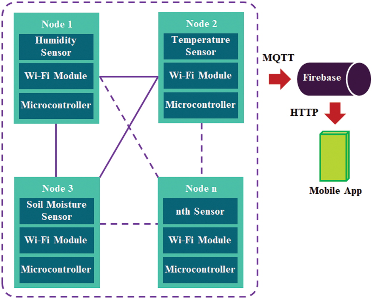
Figure 4: WSNs configuration

The hardware structure diagram, which is a representation of Fig. 4, can be seen in Fig. 5, where the nodes of the humidity, temperature and soil moisture sensors are connected to each other. Firebase, a cloud database platform, receives data for transmission to Android-based mobile gadgets.

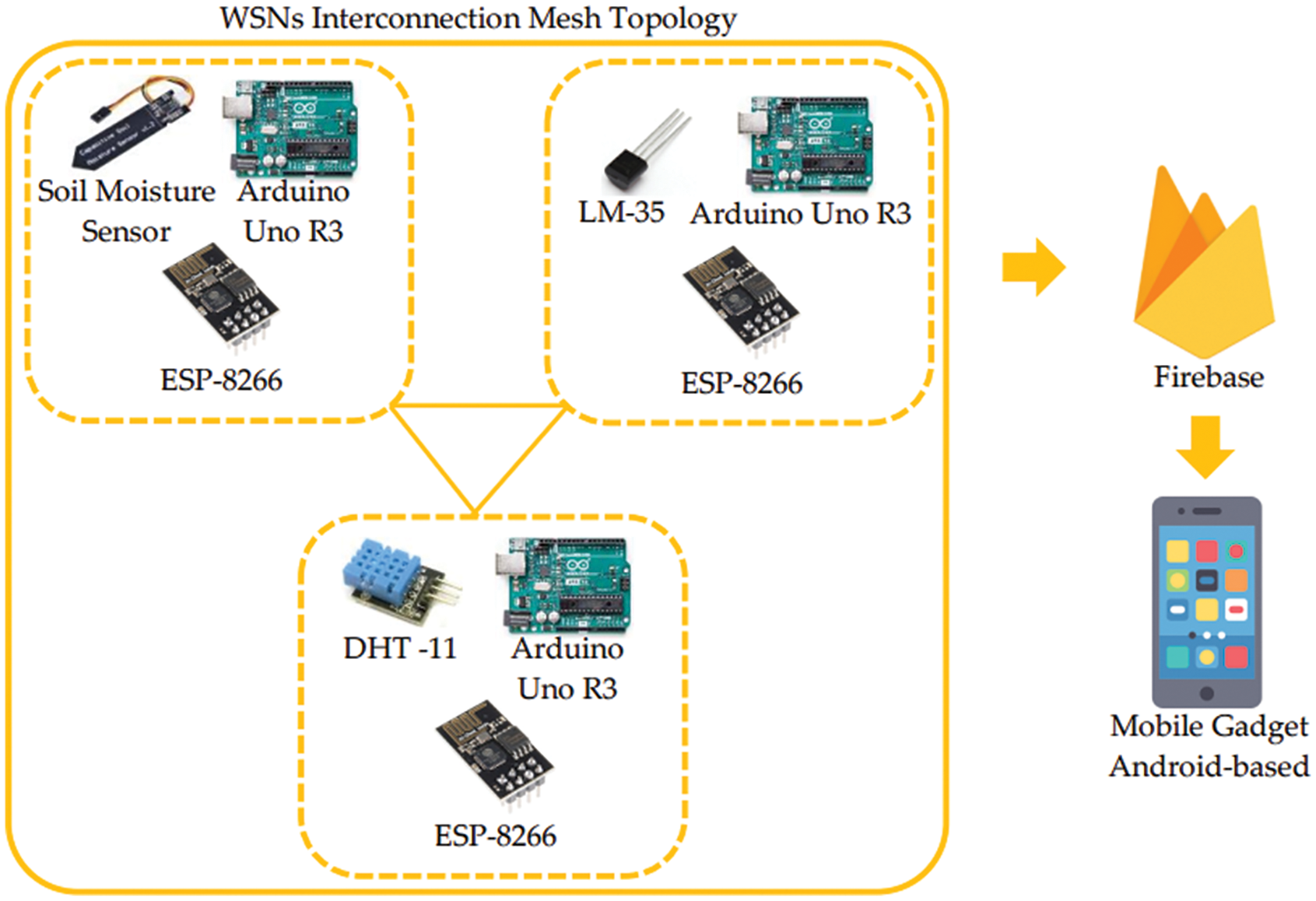
Figure 5: Hardware structure diagram

3.3 Construction of Deep Reinforcement Learning (DRL)

As explained in the previous section, this study uses DRL in data processing by combining reinforcement learning and deep neural networks (DNN) because the system works based on the agent’s performance in processing state into action. Specifically, the DNN model implemented in the DRL architecture is multi-layer perceptrons (MLP) which has the function of carrying out computational Q-value process Q-learning. In this study, MLP has the advantage of handling general data such as numerical and text data, also conducting the computational efficiency regarding less parameters involved in the computational process. Model scenarios need to be made to become basic knowledge for agents in making decisions. Scenario refers to Q-learning, which consists of state and action. In the Q-learning development stage, the state-action scenario uses DNN to produce optimal results, so it is necessary to conduct a training model. The environment is the basis for providing the initial conditions to the agent in the form of state (s), which consists of conditions of humidity (H), temperature (T), and soil moisture (M) which become a set s = [H, T, M]. For example, the results of sensor readings in real-time conditions for the mango plant environment for humidity are 56%, temperature 28°C, and soil moisture is 45%, then the state parameter is represented by s = [56, 28, 45], then s is forwarded to the Agent as the basis for data processing. DNN works to process s data through a layer consisting of neurons in the input layer, hidden layer, and output layer. This study uses four layers including 1 input layer, 2 hidden layers, and 1 output layer. Policy (π) synergizes with processing neurons in the DNN to map s to the action (a). a produced from DNN processing is a recommendation for the environmental conditions of the mango plantation environment whether they are in “optimal”, “sub-optimal” or “not-optimal” conditions. Reward (r) is feedback from the environment to the Agent on how optimal the resulting action is, and becomes a consideration for the Agent to determine the next a, apart from based on s. Fig. 6 represents the DRL process flow in this study.

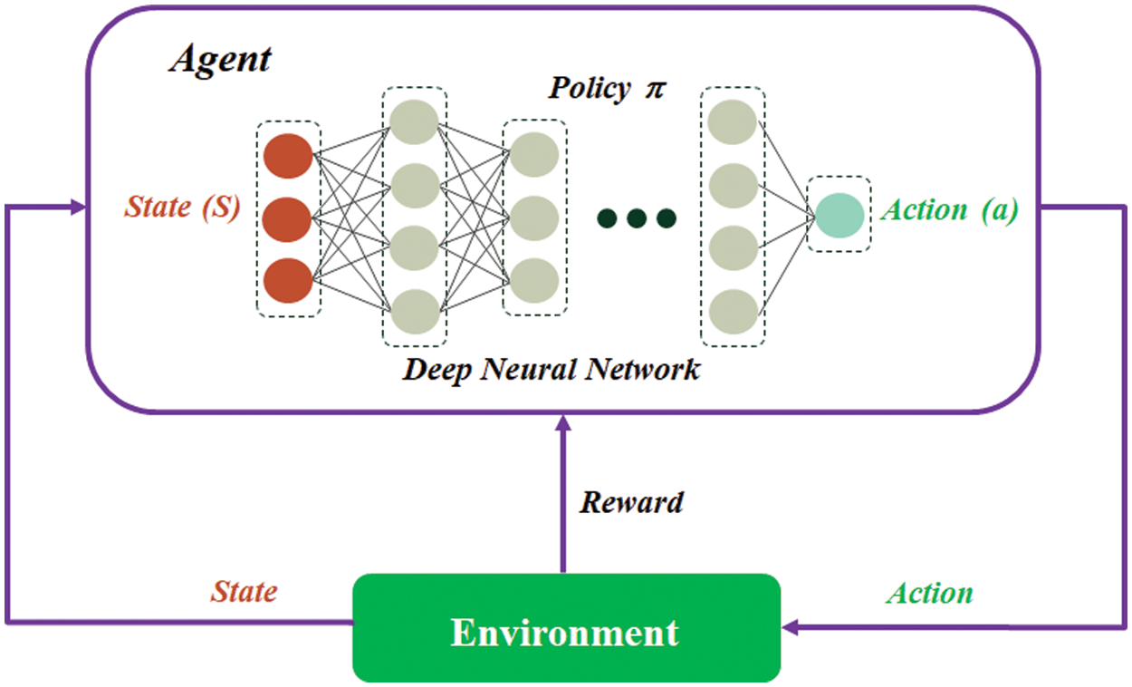
Figure 6: Process of DRL in the study

Technically, the DNN model implemented in DRL is a deep Q-network (DQN) that works based on a Q-value (action-value function) based on the given state. The state is a set of datasets consisting of scenarios of “optimal” and “not optimal” conditions based on humidity, temperature, and soil moisture parameters. In DQN, initialization of Q-values is carried out based on a predetermined Q-function, then the selection of action a is based on state s. Reward r is based on environmental conditions read by the environment, which consists of humidity (H), temperature (T), and soil moisture (M). If the parameters meet the “optimal” conditions, then r will give a positive value, otherwise, r will give a negative value. After giving r, there is an updating of the Q-value which refers to the following Bellman formulation in Eq. (6):

Qnew(s, a)=Q(s, a)+α[r(s, a)+γ×maxQ′(s′, a′)−Q(s,a)](6)

In Eq. (6) above, the updated Q-value consisting of s [H, T, M] and a is represented by Qnew(s, a). The formulation is carried out with the current Q-value, which is indicated by Q(s, a) plus the sum of the rewards r(s, a) with a discount rate γ, which is multiplied by the highest value of the Q-value in the form of maxQ′(s′, a′) and reduced by current Q-value Q(s, a). A learning rate α is implemented to seek model optimization in determining Qnew(s, a). Meanwhile, γ is a value between 0 and 1 [0, 1], which represents how much the agent determines the future reward. DQN works through a neural network to produce optimal and accurate actions. The state is the basis for a neural network to perform computational processes.

3.4 Construction of Deep Q-Network (DQN) Modeling by Q-Value Dataset

As an initial parameter, a Q-value is needed which contains a dataset of parameter scenarios for “optimal”, “sub-optimal” and “not-optimal” conditions based on humidity, temperature, and soil moisture “optimal” conditions are the normal conditions required by a mango plantation to grow optimally by looking at the conditions of humidity, temperature, and soil moisture [35]. Table 2 represents the “optimal” environmental conditions for mango plantation.

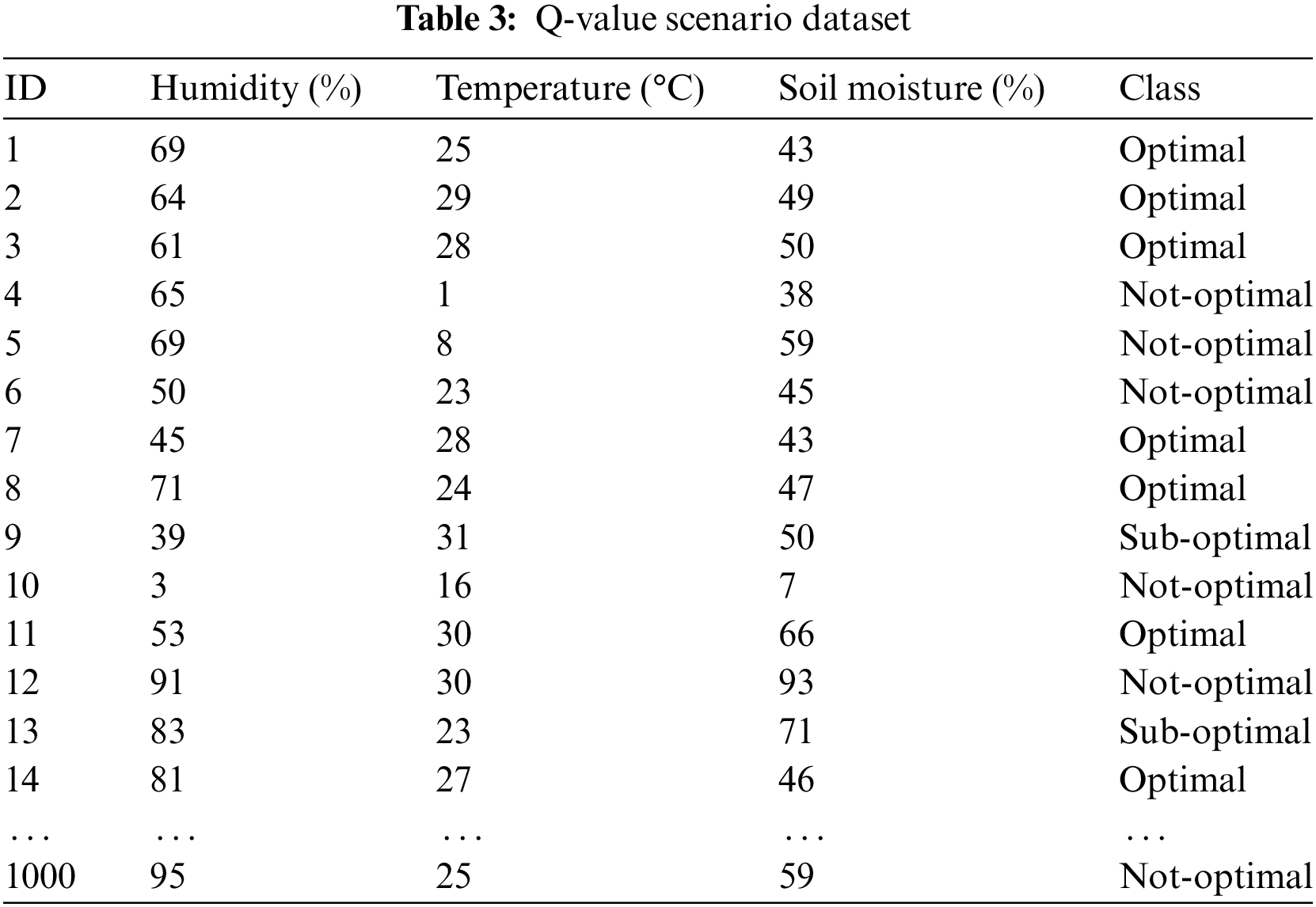
From the optimal conditions referred to in Table 2 above, a model scenario is generated with “optimal,” “sub-optimal,” and “not-optimal” class conditions. If all parameters match the optimal conditions in Table 2, then the class label is “optimal.” Otherwise, if the parameter is less than or exceeds the optimal value by 1%~2%, then it is included in the “sub-optimal” class condition. Meanwhile, the condition is “not-optimal” if the parameters exceed the “sub-optimal” condition. This model scenario is a dataset that will later be used as an initial parameter of how the agent explores its environment to produce an action in the form of recommendations for whether the environmental conditions are “optimal,” “sub-optimal,” or “not-optimal.” The scenarios that were implemented amounted to 1500 data including “optimal,” “sub-optimal” and “not-optimal” conditions of 500, 500, and 500 data, respectively. Table 3 represents the dataset scenarios developed in this study.

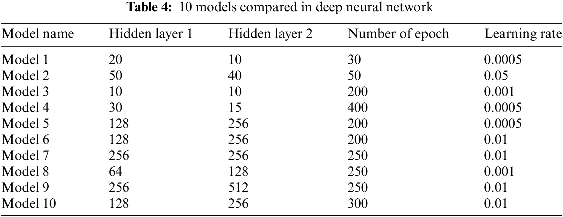
Previous studies related to modeling in agriculture were conducted by some researchers. Youness et al. [36] implemented machine learning in the field of agriculture for smart irrigation. The implemented model is a classification model task with an accuracy level of approximately 90%. Worachairungreung et al. [37] used random forest modeling in oil palm plantations to control soil index, water index, and vegetation index. Based on the modeling evaluation, the resulting accuracy is 93.41%. In this study to produce the best accuracy, it will implement deep learning modeling through deep neural networks (DNN) to the Q-value scenario dataset. DNN comparison is carried out by performing hyper parameters tuning on the hidden layer, learning rate, and number of epochs. From the comparison model, it can be seen that the best value is in terms of accuracy, F1 score, precision, and recall based on the resulting confusion matrix. In this study there are 10 DNN models compared, as shown in Table 4.

3.5 Flowchart of Experimental Process

In this study, the experimental process is divided into several parts to develop an intelligent plantation monitoring system that is easy to implement, precise, and reliable, i.e., (1) validating of WSNs accuracy by ensuring that the nodes contained in WSNs produce good accuracy in environmental readings based on parameters of humidity, temperature, and soil moisture; (2) analysis of the implemented model which aims to provide the best model accuracy used in this study to produce valid and accurate output; and (3) analysis of DRL by analyzing how the agent makes decisions based on environmental parameters of the mango plant, then processes them into decision output in the form of “optimal”, “sub-optimal” or “not-optimal” environmental conditions. Fig. 7 shows the flowchart of the experimental process which begins with integrating all sensors, in this case, the humidity sensor, temperature sensor, and soil moisture sensor with Arduino Uno R3 microcontroller and Wi-Fi module. The next stage is configuring WSNs where nodes are interconnected to form a mesh topology. The process of reading the environment of mango plantations by WSNs is based on parameters of humidity, temperature, and soil moisture. The results of the readings are then analyzed by making comparisons through measurement tools. Technically, the accuracy weight is indicated by the mean absolute percentage error (MAPE) by calculating the absolute percentage error between actual result (at) and prediction result (pt), which is formulated in Eq. (7):

MAPE=1n∑t=1n|at−ptat|(7)

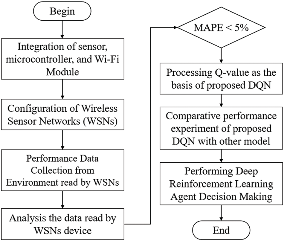
Figure 7: Flowchart of experimental process

In this case, if the MAPE is less than 5%, then the Q-value will be continued as the basis for the DQN model using deep neural network (DNN) analysis at the processing stage, and if the MAPE is equal to or greater than 5%, then processing will be carried out again by the reading of environmental data using WSNs. Q-value processing is carried out by developing dataset scenarios, which are the basis for the proposed DQN. The optimization process is carried out by hyper parameter tuning on the dataset. Next, the proposed DQN is compared with other models to see how the model developed performs. The final stage is to carry out DRL in decision-making through the user interface to see how the agent perceives the actual environment of the mango plantation, whether it is “optimal,” “sub-optimal,” or “not-optimal.”

4  Results and Discussion

4.1 Validating of WSNs Accuracy

Validating the accuracy of WSNs is conducted by collecting data from the mango plantation environment based on humidity, temperature, and soil moisture. This stage is also part of validating the performance and networking characteristics of the WSNs whether accurate or less. The data collection process is carried out in 13 different data timeframes starting at 6 a.m. to 6 p.m. every hour. At the time of data collection, the temperature was around 25°C~30°C with the weather being relatively sunny and no rain. Fig. 8 shows how the interconnection of components between microcontroller devices, Wi-Fi modules with humidity sensors, temperature sensors, and soil moisture sensors. The distance between the device and the mango plantation is 1 m. Therefore, the device can read effectively around the mango plantation environment. Soil moisture is planted on the ground with a distance of 1 m in mango plantation and the depth of planting soil moisture is 2 cm.

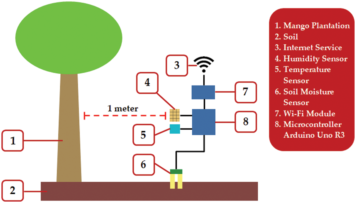
Figure 8: Environmental setup configuration

Furthermore, Fig. 9 is the actual condition of the mango plantation where the WSNs nodes are located at a radius of 1 m from the tree. Three nodes are interconnected, with a white box serving as a temperature sensor, a red box as a moisture sensor, and a blue box as a humidity sensor. Inside each box are sensor components, a microcontroller, a Wi-Fi module, and a portable power supply.

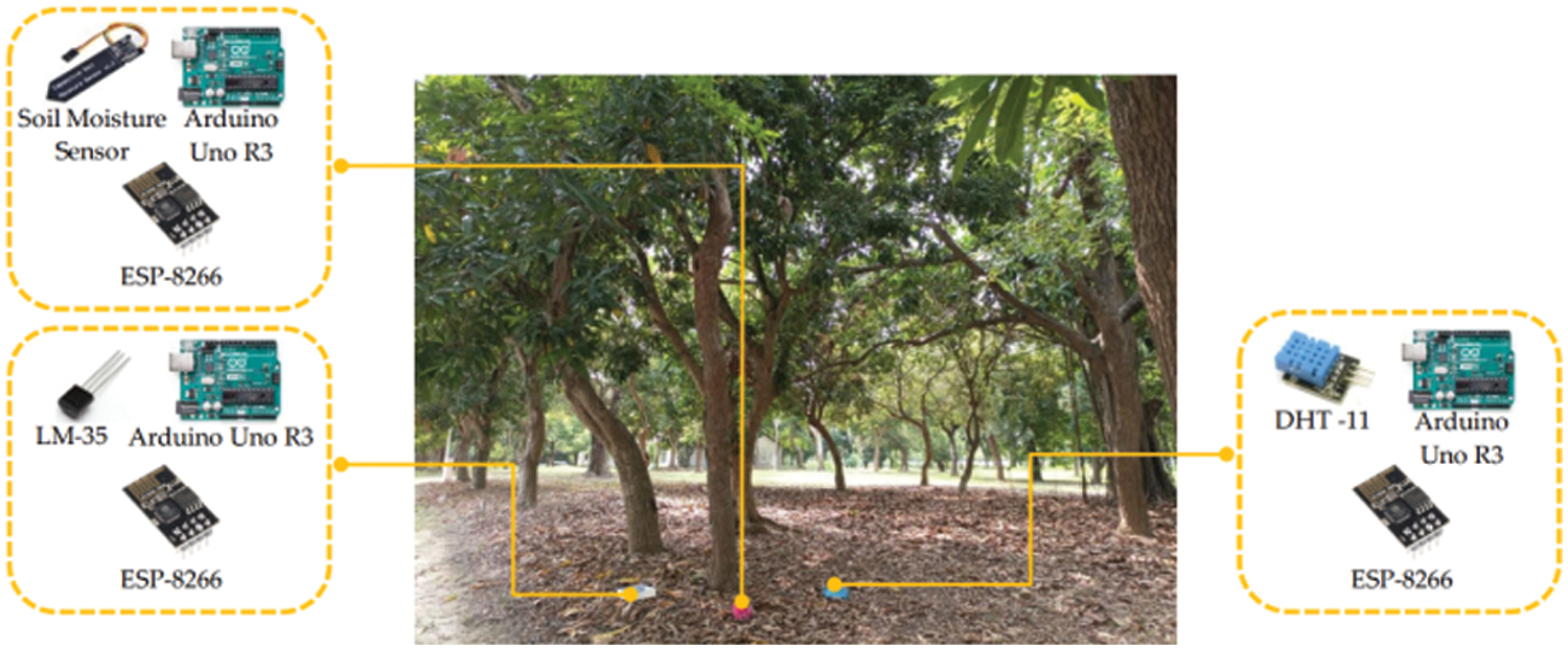
Figure 9: Actual environment condition

The process of reading data from WSNs nodes is transmitted to the Firebase cloud as real-time data. Fig. 10 is a sample of real-time data sourced from reading WSNs nodes, where there are three variables and values consisting of humidity with a value of 72 (in percentage units), soil_moisture with a value of 38 (in percentage units), and temperature with a value of 28.9 (in °C units).

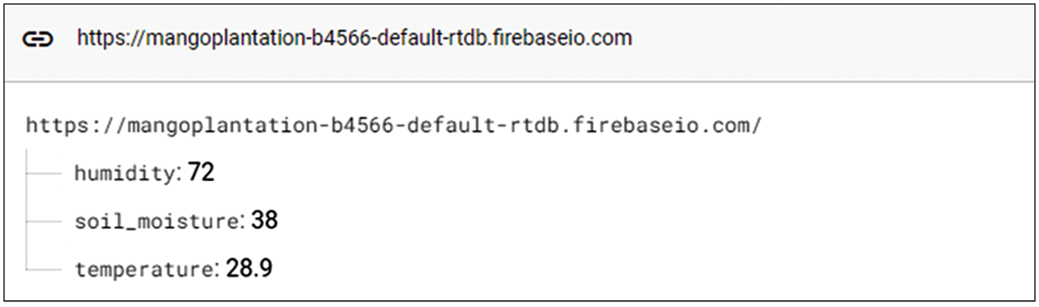
Figure 10: Actual environment condition

To measure the quality of the accuracy of readings from the device, a comparison is conducted by measuring instruments, i.e., a digital hygrometer, a digital thermometer, and a digital soil moisture analyzer. The results of the measuring instrument become a benchmark for counting the gap that is resulted by WSNs devices. The validation measurement results can be seen in Table 5, where there are 13-time frames consisting of WSNs results (device results), measurement tool results, and error percentage (EP). The humidity result is represented by H, while temperature and soil moisture are represented by T and S, respectively. There are differences and similarities between measurements produced by devices and measurement tools. For example, at measurement 06:00 a.m., the humidity produced by the device is 80%, while the measurement tools are 83%. However, there are some similarities in the calculations; for example, at a humidity of 08:00 a.m., measurements based on devices and measurement tools produce a humidity of 74%. The difference in measurement results between devices and measurement tools is an absolute gap, which then becomes the basis for calculating the error percentage (EP), which is formulated in Eq. (8):

EP=abs(m−a)a×100%(8)

where abs(m − a) is the value of the absolute gap, m is the result of calibrated measurement instruments as the standard measurement devices including a digital hygrometer, digital thermometer, and digital soil moisture to validate the result based on developed device. Meanwhile, a is the result of device measurements. So based on the calculation of error percentage (EP), the highest humidity EP is obtained at 06:00 a.m. by 3.75%. In temperature EP, the highest percentage is at 06:00 a.m., while the highest soil moisture EP is found at 08:00 a.m. and 09:00 a.m. with a percentage of 5.26%. The average EP of each parameter—humidity, temperature, and soil moisture—is 1.61%, 1.02%, and 2.25%, respectively. The mean absolute percentage error is the average value of all EP parameters, which produces 1.63% of MAPE.

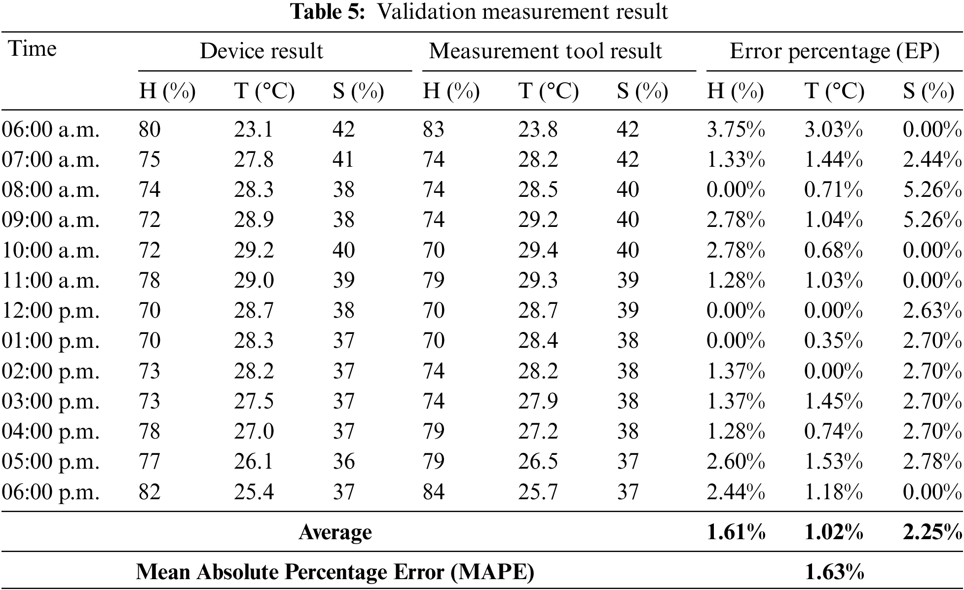
The resulting MAPE of 1.63% indicates that the results of the WSNs reading of the environment are good where in this study the threshold specified for MAPE is less than 5%, as stated in Section 3.5. Another insight with the MAPE value is that it can be seen that the accuracy percentage with the 100% formulation minus MAPE, where if MAPE is 1.63% then the accuracy percentage is 98.37%.

4.2 Analysis of Proposed DQN Model Implemented

In this study, 10 models were determined with initial parameter variations consisting of the number of neurons in layer 1, the number of neurons in layer 2, the number of epochs, and the learning rate. The activation function implemented in all modeling is “softmax” which supports multiple classes. The percentages for train data and test data are 80% and 20%, respectively. The results of modeling 10 models in the form of accuracy, F1 score, loss, memory usage, and inference time. For accuracy results and F1 scores refer to Eqs. (9) and (10), respectively.

Accuracy=(TP+TN)(TP+FP+TN+FN)(9)

F1Score=2×(P×R)(P+R)(10)

Eq. (9) is an accuracy formulation where the sum of true positives (TP) and true negatives (TN) is divided by all data consisting of false positives (FP), false negatives (FN), TP, and TN. Meanwhile, the F1 score is resulted from precision (P) multiplied by recall (R) and then divided by the sum of P and R. The results of these calculations are then multiplied by 2. P is generated by calculating TP divided by the sum of TP and FP, while R is TP divided by the sum of TP and FN. Table 6 shows the modeling results of 10 models where the accuracy range is from 64.8% to 97.6%. The lowest accuracy is found in model 2 with a percentage of 64.6% and an F1 score of 0.70. Referring to Section 3.4, model 2 has neurons in hidden layer 1 with a value of 50, hidden layer 2 with a value of 40, number of epochs of 50, and a learning rate of 0.05. Loss commonly referred to as the “loss function” shows how much the mismatch between the predicted output from machine learning modeling and the expected output. So the smaller the resulting loss, the more precise the model is built. In model 2 it can be seen that the loss is 0.58.

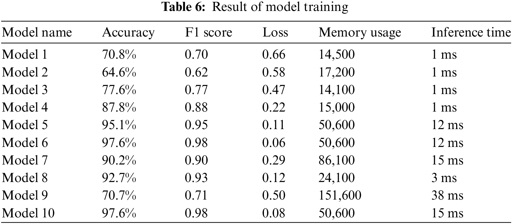
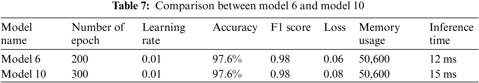
The highest accuracy in Table 6 is found in model 6 and model 10 with a percentage of 97.6% with the F1 score having the same value of 0.98. So in this case it is necessary to consider other things such as the value of the loss function. In model 6, the resulting loss function is 0.06 while model 10 shows 0.08. From the aspect of memory usage, both have the same value, that is 50,600. The inference time, which represents how long the model takes to perform the computational process, shows that model 6 and model 10 have an inference time of 12 and 15 ms, respectively. Based on these considerations, it is evident that model 6 has better efficiency than model 10. In summary, Table 7 shows a comparison between model 6 and model 10.

In order to validate the performance of the proposed DQN developed through Q-value, a comparative experiment was carried out with other models, i.e., individual Q-learning (IRL), uniform coverage (UC), and Naïve Bayes classifier (NBC). Initial parameters in the experimental process include an epoch number of 200, a learning rate of 0.01, and a batch size of 32. Table 8 represents the performance results of the trained model. There are four evaluation metrics, i.e., accuracy, recall, precision, and F1 score. Of the four models, the proposed DQN has a higher performance score compared to other models, where the accuracy value is 97.60%, recall is 0.970, precision is 0.974, and F1 score is 0.972. Overall, Fig. 11 represents the visualization of the performance model. In Fig. 11d, the highest F1 score is in the proposed DQN, while the lowest F1 score is in the IRL model. The UC model has an F1 score that is almost close to the proposed DQN.

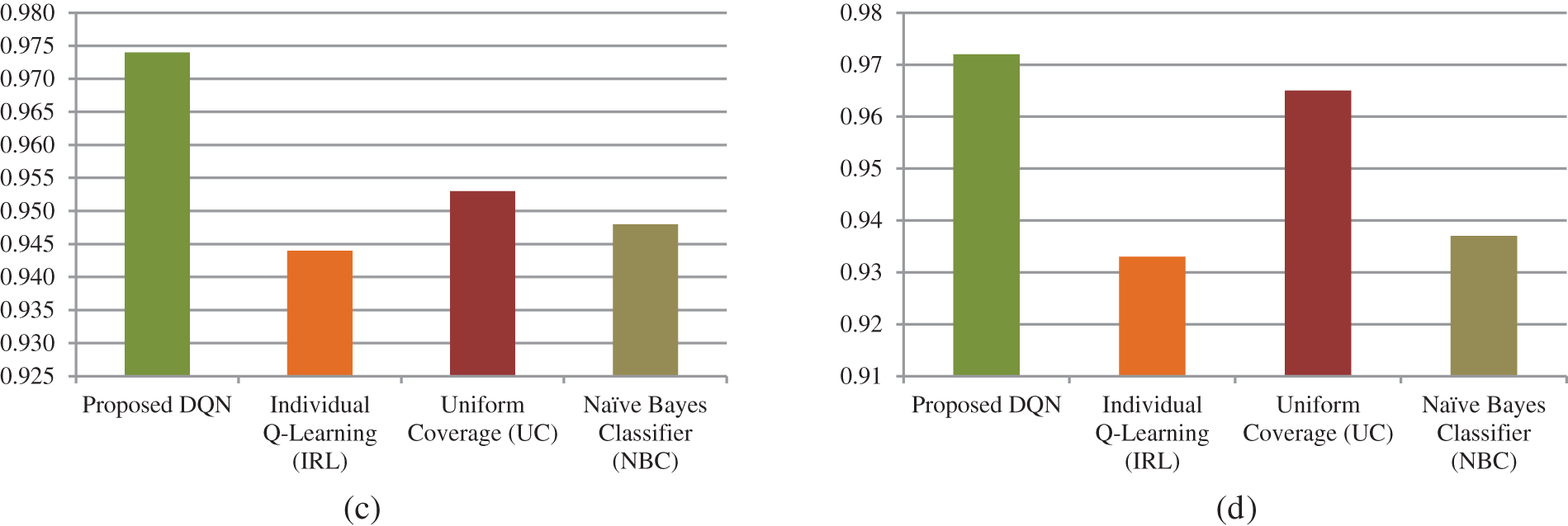
Figure 11: Model performance result. (a) Accuracy. (b) Recall. (c) Precision. (d) F1 score

Comparative analysis is also conducted to the existing previous study, which was conducted by Farkhodov et al. [38] by implementing DRL Tf-agent-based for the agricultural fields to track the unreal game engine in AirSim block simulation under different conditions and weather changes. Experimental stages indicate performance efficiency was obtained at an epoch of 400 and had achieved an accuracy percentage of 92%. Ahmadi et al. [39] employed DQRE-SCnet model as the deep-Q-reinforcement learning based on spectral clustering. The method integrates the federated learning strategy in order to distribute the node network in the cloud platform. The experimental simulation employs three different datasets including MNIST, fashion mnist, and CIFAR-10 which gain the accuracy percentage of 92.30%, 88.13%, and 58.38%, respectively. Said et al. [40] developed DQLRFMG which is the combination of several methods including deep-Q-learning, logistic regression, and deep forest multivariate classification to grade the fruit. The experiment involves three different datasets: Kaggle-fruit360, Front phenotyping dataset, and ImageNet sample. The experimental result indicates that the proposed model has the improvement of accuracy, precision, recall, and AUC. Fig. 12 represents the comparative analysis of the proposed method in this study compared to the previous study explained above.

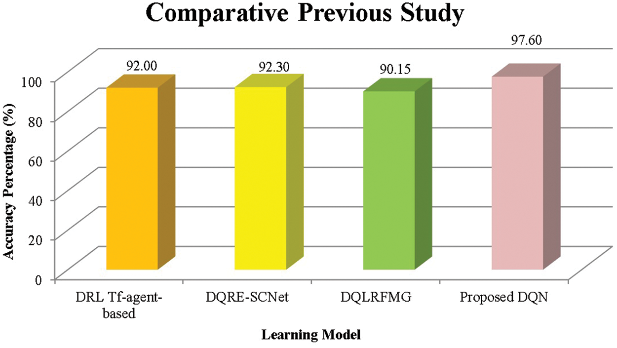
Figure 12: Comparative previous study

4.3 Experiment of Deep Reinforcement Learning

The user interface is made to represent how the agent in DRL works to produce output based on humidity, temperature, and soil moisture parameters. Fig. 13 shows the design of the user interface with part (a) which is the main menu and part (b) the result menu user interface which has 3 displays of real-time conditions from the mango plantation and information columns on the current state of the mango plantation environment based on three parameters. Android-based system platform with minimum specification Android version 4.0, 1 giga-byte random access memory, 100 megabytes of storage, and 1 GHz processor. The purpose of Fig. 13 is to show how the user interface built on the DRL system is used to facilitate interaction between the user and the system, where the display of humidity value, temperature value, and soil moisture value is the real-time condition of the mango plantation environment. Users can see how changes in environmental conditions through these three parameters. Meanwhile, at the bottom of the resulting menu, there are two recommendations for the decision of the DRL agent based on three parameters, where the system will decide whether the conditions of the three parameters are “optimal”, “sub-optimal” or “not-optimal”.

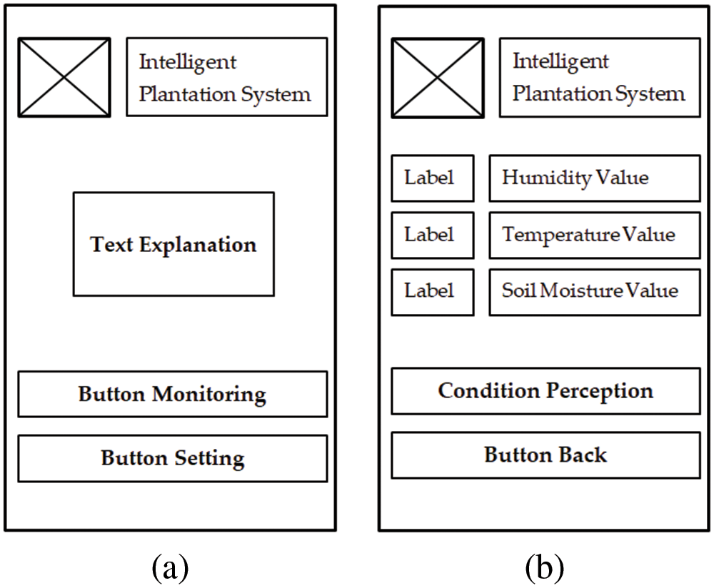
Figure 13: User interface. (a) Main menu. (b) Result menu

Furthermore, to assess the quality of the implemented modeling, a test scenario was created. In this study, there were 22 test scenarios with data collection under different conditions and varying characteristics of humidity, temperature, and soil moisture. The 22 test scenarios represent various conditions in the mango planting environment, for example in scenario 19 where the expected value is “not-optimal” with the parameters humidity is 48%, temperature is 20°C, and soil moisture is 55%. The data collection process was carried out at a temperature value of 20°C (around 3~4 a.m.) with random humidity and soil moisture conditions. Likewise scenario 18, with an expected value of “not optimal”, where soil moisture is conditioned to a value of 74% through over-watering, but with random humidity and temperature conditions. So the total of 22 test scenarios on the system that represent a variety of environmental conditions whether “optimal”, “sub-optimal” or “not-optimal” is representative to demonstrate the effectiveness of the method. Table 9 shows the test results of the DRL system where there are three parameter columns, the expected value is the basis for comparison of the system being tested, as well as the DRL system column which is the result of system testing. In the test scenario conditions are divided into 12 data records for “optimal” conditions, 5 data records for “sub-optimal” conditions, and 5 data records for “not-optimal” conditions. Data collection was carried out randomly in several places in the mango plantation environment with variations in humidity, temperature, and soil moisture conditions.

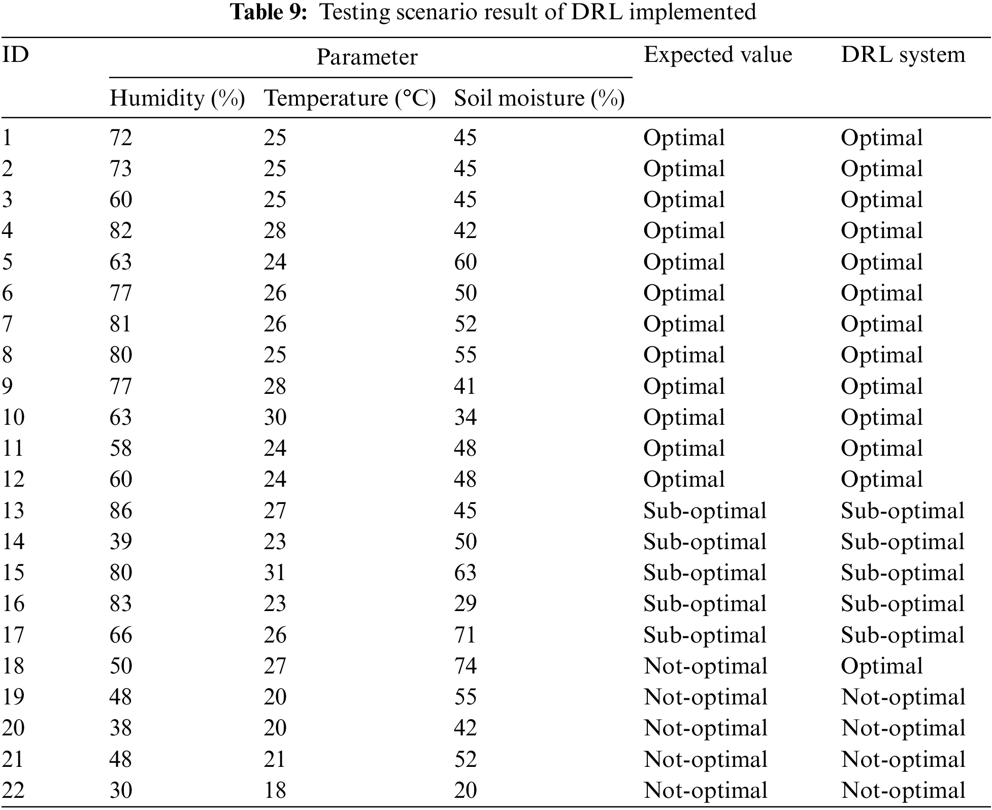
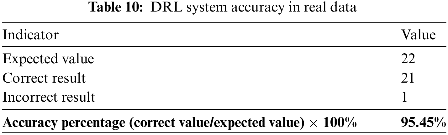
From the test results in Table 9, there is 1 test result with an incorrect result which is at test ID 18. The expected value, which is a benchmark for comparison, is listed as “not-optimal”, because the soil moisture exceeds the specified threshold. Meanwhile, the results of the DRL system test on the environmental conditions of the mango plantation showed “optimal” results. If it is further analyzed, this can be caused by an error generated by the system that reads data close to the specified threshold. Overall the test results, the DRL system has the accuracy of the test results in as many as 21 scenarios out of 22 scenarios. So if it is presented, it will produce an accuracy of 95.45%. Table 10 represents the details of the accuracy of the DRL system test on the mango plantation environment.

4.4 Evaluation of Cost Efficiency

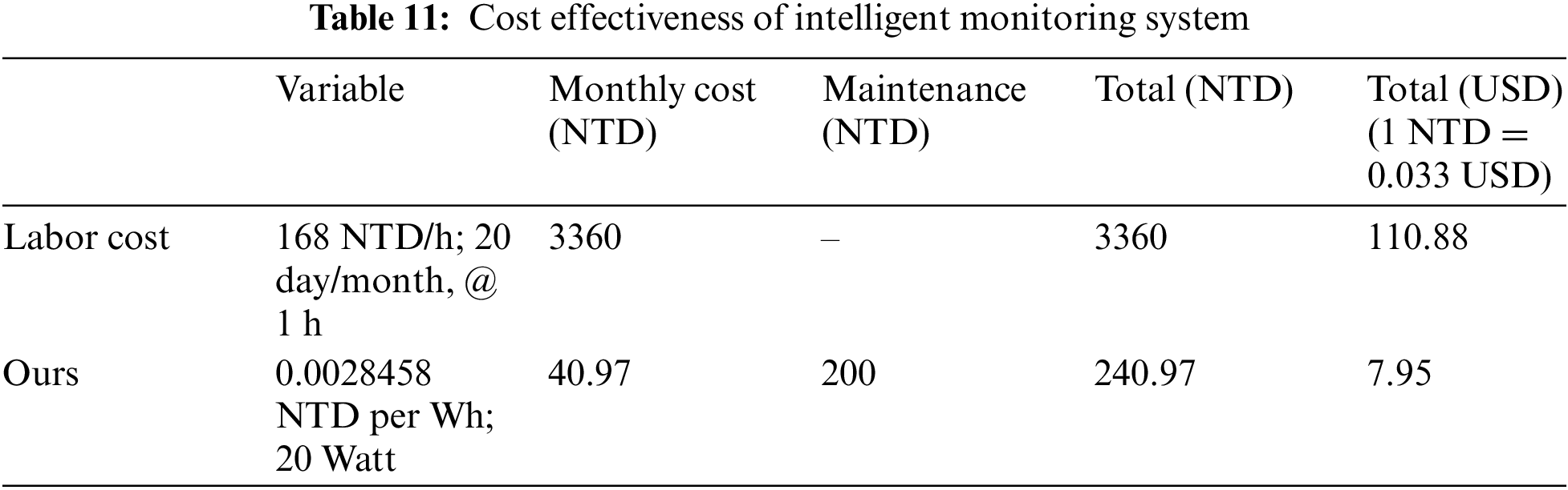
In evaluating cost efficiency, the components used are variables that are charged in the use of intelligent monitoring system costs compared to labor costs. Thus, the evaluation of cost efficiency does not discuss how much capital costs are charged to build an intelligent plantation monitoring system. When compared with labor costs, based on data from the Ministry of Labor in Taiwan, the hourly basic wage is 168 NTD [41]. As a comparison, it is assumed that the average working hour for monitoring workers is one hour per day with a working day of 5 days so that a week is 5 working days or a month is 20 working days. The total cost of labor is 168 NTD multiplied by 20 working days and one hour per day, resulting in a minimum cost of 3360 NTD per month which is charged to labor costs to carry out routine plantation monitoring.

Meanwhile, in the use of an intelligent monitoring system, the cost component charged is the use of electric power and maintenance costs. The maximum power in this intelligent system is 20 W assuming use for 24 h and used for 1 month (30 days), so the accumulated monthly usage hours is 24 h multiplied by 30 days resulting in 720 h of use for 1 month. So if used in a month, then 20 W multiplied by 720 h. Electric power usage based on Taiwan’s standard electricity cost is 2.8458 NTD per kilowatt-hour (kWh) [42]. Because the use of electric power is 20 W, the cost of electricity needs to be converted per watt-hour (Wh) to 0.0028458 per Wh. So if it is calculated the cost of electricity for a month is 720 h multiplied by 20 W multiplied by the electricity rate of 0.0028458 per Wh, resulting in an electricity cost of 40.97 NTD per month. As for the maintenance costs required for component replacement and calibration, it is assumed to be 200 NTD, so the overall cost of electricity and maintenance for the intelligent plantation system is 240.97 NTD. Table 11 describes the cost-effectiveness evaluation between the intelligent plantation monitoring system and labor costs.

5  Conclusion

The intelligent plantation monitoring system provides convenience in plantation management, especially mango plantations, through artificial intelligence technology that is accurate, easy to implement, reliable, and low-cost. A series of steps are carried out to produce precise device quality, which begins with testing the WSNs to find out the quality of the sensors used. At this stage, it produces a mean absolute percentage error (MAPE) of 1.63% or an accuracy of 98.37%. The Q-value dataset uses deep neural network modeling as a basis for the proposed DQN model, which will be implemented in the DRL agent. Comparative experiments to see the proposed DQN performance were carried out on individual Q-learning (IRL), uniform coverage (UC), and Naïve Bayes classifier (NBC). Based on the comparative experiment results, it was found that the proposed DQN had higher scores on the four evaluation metrics of accuracy, recall, precision, and F1 score. Based on the experimental results in real data, the intelligent plantation monitoring system has the advantage that, based on device testing, it can read the environmental conditions of the mango plantation with an accuracy of 95.45%. Meanwhile, in cost efficiency aspect, when compared to labor costs, the monthly cost of the intelligent plantation monitoring system is much more efficient.

However, the proposed method which employs the value function mechanism called DQN has limitations especially in computational cost if it is integrated with a huge amount of data. As the prevention suggestion to address this issue, data could be parted into small amounts of batch data and the model can conduct computational processes in parallel to obtain the memory consumption efficiency. As a continuation of development, the intelligent plantation monitoring system can be used as the basis for an integrated intelligent plantation system, where the system can provide the entire plantation process, starting from monitoring, maintenance, applying fertilizers and organic pesticides, harvesting processes, and post-harvesting processes. The system improves the quality of agricultural yields by combining artificial intelligence technology, which produces accurate, precise, easy-to-implement, reliable, and low-cost data processing.

Acknowledgement: This research was supported by the Department of Electrical Engineering at the National Chin-Yi University of Technology. The authors would like to thank the National Chin-Yi University of Technology, Takming University of Science and Technology, Taiwan, for supporting this research.

Funding Statement: The authors received no specific funding for this study.

Author Contributions: Conceptualization, Wen-Tsai Sung and Indra Griha Tofik Isa; methodology, Indra Griha Tofik Isa; software, Indra Griha Tofik Isa; validation, Sung-Jung Hsiao; formal analysis, Wen-Tsai Sung; writing—original draft preparation, Indra Griha Tofik Isa; writing—review and editing, Sung-Jung Hsiao. All authors reviewed the results and approved the final version of the manuscript.

Availability of Data and Materials: Data sharing does not apply to this article as no datasets were generated or analyzed during the current study.

Ethics Approval: Not applicable.

Conflicts of Interest: The authors declare that they have no conflicts of interest to report regarding the present study.

References

1. M. Y. Wu and C. K. Ke, “Development and application of intelligent agricultural planting technology—The case of tea,” in Proc. IS3C 2020, Taichung, Taiwan, 2020, pp. 43–44. [Google Scholar]

2. N. Roslan, A. A. Aznan, R. Ruslan, M. N. Jaafar, and F. A. Azizan, “Growth monitoring of harumanis mango leaves (Mangifera indica) at vegetative stage using SPAD meter and leaf area meter,” in Proc. MEBSE, Bogor, Indonesia, 2018, pp. 1–6. [Google Scholar]

3. M. Cruz, S. Mafra, E. Teixeira, and F. Figueiredo, “Smart strawberry farming using edge computing and IoT,” Sensors, vol. 22, no. 15, pp. 1–33, 2022, Art. no. 5866. doi: 10.3390/s22155866. [Google Scholar] [PubMed] [CrossRef]

4. K. Kipli et al., “Deep learning applications for oil palm tree detection and counting,” Smart Agric. Technol., vol. 5, pp. 1–8, 2023, Art. no. 100241. doi: 10.1016/j.atech.2023.100241. [Google Scholar] [CrossRef]

5. A. Barriga, J. A. Barriga, M. J. Monino, and P. J. Clemente, “IoT-based expert system for fault detection in Japanese Plum leaf-turgor pressure WSN,” Internet of Things, vol. 23, no. 1, pp. 1–33, 2023, Art. no. 100829. doi: 10.1016/j.iot.2023.100829. [Google Scholar] [CrossRef]

6. M. F. Ibrahim et al., “IoT monitoring system for fig in greenhouse plantation,” J. Adv. Res. Appl. Sci. Eng. Technol., vol. 31, no. 2, pp. 298–309, 2023. doi: 10.37934/araset.31.2.298309. [Google Scholar] [CrossRef]

7. V. Viswanatha et al., “Implementation of IoT in agriculture: A scientific approach for smart irrigation,” in IEEE 2nd MysuruCon, Mysuru, India, 2022, pp. 1–6. [Google Scholar]

8. S. B. Dhal et al., “An IoT-based data-driven real-time monitoring system for control of heavy metals to ensure optimal lettuce growth in hydroponic set-ups,” Sensors, vol. 23, pp. 1–11, 2023, Art. no. 451. doi: 10.3390/s23010451. [Google Scholar] [PubMed] [CrossRef]

9. I. Belupu, C. Estrada, J. Oquelis, and W. Ipanaque, “Smart agriculture based on WSN and Node.js for monitoring plantations in rural areas: Case region Piura, Peru,” in Proc. 2021 IEEE CHILEAN, CHILECON 2021, Valparaiso, Chile, 2021, pp. 1–6. [Google Scholar]

10. H. Benyezza, M. Bouhedda, R. Kara, and S. Rebouh, “Smart platform based on IoT and WSN for monitoring and control of a greenhouse in the context of precision agriculture,” Internet of Things, vol. 23, pp. 1–18, 2023, Art. no. 100830. doi: 10.1016/j.iot.2023.100830. [Google Scholar] [CrossRef]

11. A. R. Muhammad, O. Setyawati, R. A. Setyawan, and A. Basuki, “WSN based microclimate monitoring system on porang plantation,” in Proc. 2018 EECCIS 2018, Batu, Indonesia, 2018, pp. 142–145. [Google Scholar]

12. G. G. R. De Castro et al., “Adaptive path planning for fusing rapidly exploring random trees and deep reinforcement learning in an agriculture dynamic environment UAVs,” Agriculture, vol. 13, no. 2, pp. 1–25, 2023, Art. no. 354. doi: 10.3390/agriculture13020354. [Google Scholar] [CrossRef]

13. A. Din, M. Yousoof, B. Shah, M. Babar, F. Ali and S. Ullah, “A deep reinforcement learning-based multi-agent area coverage control for smart agriculture,” Comput. Electr. Eng., vol. 101, pp. 1–11, 2022, Art. no. 108089. doi: 10.1016/j.compeleceng.2022.108089. [Google Scholar] [CrossRef]

14. Y. Li et al., “Research on winter wheat growth stages recognition based on mobile edge computing,” Agriculture, vol. 13, no. 3, pp. 1–16, 2023, Art. no. 534. doi: 10.3390/agriculture13030534. [Google Scholar] [CrossRef]

15. N. Zhou, “Intelligent control of agricultural irrigation based on reinforcement learning,” in Proc. ICEMCE, Xi’an, China, 2020, pp. 1–6. [Google Scholar]

16. S. S. Afzal, A. Kludze, S. Karmakar, R. Chandra, and Y. Ghasempour, “AgriTera: Accurate non-invasive fruit ripeness sensing via sub-terahertz wireless signals,” in 29th Annu. Int. Conf. Mobile Comput. Netw. (ACM MobiCom’23), Madrid, Spain, 2023, pp. 1–15. [Google Scholar]

17. P. Aryai et al., “Real-time health monitoring in WBANs using hybrid Metaheuristic-Driven Machine Learning Routing Protocol (MDML-RP),” AEU-Int. J. Electron. Commun., vol. 168, pp. 1–15, 2023, Art. no. 154723. doi: 10.1016/j.aeue.2023.154723. [Google Scholar] [CrossRef]

18. S. Memarian et al., “TSFIS-GWO: Metaheuristic-driven takagi-sugeno fuzzy system for adaptive real-time routing in WBANs,” Appl. Soft Comput., vol. 155, pp. 1–19, 2024, Art. no. 111427. doi: 10.1016/j.asoc.2024.111427. [Google Scholar] [CrossRef]

19. A. Kocian and L. Incrocci, “Learning from data to optimize control in precision farming,” Stats, vol. 3, no. 3, pp. 239–245, 2020. doi: 10.3390/stats3030018. [Google Scholar] [CrossRef]

20. R. Tao et al., “Optimizing crop management with reinforcement learning and imitation learning,” in Proc. Int. Joint Conf. Auton. Agents Multiagent Syst., AAMAS, London, UK, 2023, pp. 2511–2513. [Google Scholar]

21. R. J. Boucherie and N. M. V. Dijk, General theory. in Markov Decision Processes in Practice. Cham, Switzerland: Springer International Publishing AG, pp. 3–5, 2017. Accessed: Dec. 20, 2023. [Online]. Available: https://link.springer.com/book/10.1007/978-3-319-47766-4 [Google Scholar]

22. Z. Pan, G. Wen, Z. Tan, S. Yin, and X. Hu, “An immediate-return reinforcement learning for the atypical Markov decision processes,” Front. Neurorobot., vol. 16, pp. 1–20, 2022. doi: 10.3389/fnbot.2022.1012427. [Google Scholar] [PubMed] [CrossRef]

23. R. S. Sutton and A. G. Barto, Reinforcement Learning: An Introduction, 2nd ed. Cambridge, USA: The MIT Press, pp. 57–62, 2018. [Google Scholar]

24. L. Xia, X. Guo, and X. Cao, “A note on the existence of optimal stationary policies for average Markov decision processes with countable states,” Automatica, vol. 151, pp. 1–8, 2023, Art. no. 110877. doi: 10.1016/j.automatica.2023.110877. [Google Scholar] [CrossRef]

25. R. Singh, A. Gupta, and N. B. Shroff, “Learning in constrained markov devision processes,” IEEE Trans. Control Netw. Syst., vol. 10, no. 1, pp. 441–453, 2023. doi: 10.1109/TCNS.2022.3203361. [Google Scholar] [CrossRef]

26. V. Anantharam, “Reversible Markov decision processes and the Gaussian free field,” Syst. Control Lett., vol. 169, pp. 1–8, 2022, Art. no. 105382. doi: 10.1016/j.sysconle.2022.105382. [Google Scholar] [CrossRef]

27. G. De Giacomo, M. Favorito, F. Leotta, M. Mecella, and L. Silo, “Computers in industry digital twin composition in smart manufacturing via Markov decision processes,” Comput. Ind., vol. 149, pp. 1–10, 2023, Art. no. 103916. doi: 10.1016/j.compind.2023.103916. [Google Scholar] [CrossRef]

28. M. Morales, Balancing immediate and long-term goals. in Grokking Deep Reinforcement Learning, 1st ed. Shelter Island, NY, USA: Manning Publication Co., pp. 66–77, 2020. [Google Scholar]

29. P. Winder, “Markov decision process, dynamic programming, and Monte Carlo methods,” in Reinforcement Learning Industrial Application of Intelligent Agents, 1st ed. Sebastopol, USA: O’Reilly Media, Inc., pp. 25–57, 2021. [Google Scholar]

30. L. Graesser and W. L. Keng, “Reinforce,” in Foundation of Deep Reinforcement Learning: Theory and Practice in Python. Boston, USA: Addison Wesley Publishing, Inc., pp. 26–30, 2019. [Google Scholar]

31. Y. Matsuo et al., “Deep learning, reinforcement learning, and world models,” Neural Netw., vol. 152, pp. 267–275, 2022. [Google Scholar] [PubMed]

32. E. A. Elaziz, R. Fathalla, and M. Shaheen, “Deep reinforcement learning for data‐efficient weakly supervised business process anomaly detection,” J. Big Data, vol. 10, no. 33, pp. 1–35, 2023. doi: 10.1186/s40537-023-00708-5. [Google Scholar] [CrossRef]

33. Y. Hou, W. Gu, W. Dong, and L. Dang, “A deep reinforcement learning real-time recommendation model based on long and short-term preference,” Int. J. Comput. Intell. Syst., vol. 16, no. 4, pp. 1–14, 2023. [Google Scholar]

34. Z. Q. Mohammed Ali and S. T. Hasson, “Simulating the wireless sensor networks coverage area in a mesh topology,” in Proc. 4th ICASE, Kurdistan Region, Iraq, 2022, pp. 387–390. [Google Scholar]

35. Food and Agriculture Organization of The United Nations, Food and Agriculture Microdata Catalogue (FAM). Rome, Italy: FAO-UN, 2023. Accessed: Dec. 23, 2023. [Online]. Available: https://www.fao.org/food-agriculture-microdata/en/ [Google Scholar]

36. H. Youness, G. Ahmed, and B. El Haddadi, “Machine learning-based smart irrigation monitoring system for agriculture applications using free and low-cost IoT platform,” in Proc. ICM, Casablanca, Morocco, 2022, pp. 189–192. [Google Scholar]

37. M. Worachairungreung, K. Thanakunwutthirot, and N. Kulpanich, “A study on oil palm classification for ranong province data fusion and machine learning algorithms,” Geogr. Technica, vol. 18, no. 1, pp. 161–176, 2023. doi: 10.21163/GT_2023.181.12. [Google Scholar] [CrossRef]

38. K. Farkhodov, S. H. Lee, J. Platos, and K. R. Kwon, “Deep reinforcement learning tf-agent-based object tracking with virtual autonomous drone in a game engine,” IEEE Access, vol. 11, pp. 124129–124138, 2023. doi: 10.1109/ACCESS.2023.3325062. [Google Scholar] [CrossRef]

39. M. Ahmadi et al., “DQRE-SCnet: A novel hybrid approach for selecting users in federated learning with deep-Q-reinforcement learning based on spectral clustering,” J. King Saud Univ.-Comput. Inf. Sci., vol. 34, no. 9, pp. 7445–7458, 2022. doi: 10.1016/j.jksuci.2021.08.019. [Google Scholar] [CrossRef]

40. A. G. Said and B. Joshi, “DQLRFMG: Design of an augmented fusion of deep Q learning with logistic regression and deep forests for multivariate classification and drading of fruits,” Int. J. Recent Innov. Trends Comput. Commun., vol. 11, no. 7, pp. 270–281, 2023. doi: 10.17762/ijritcc.v11i7.7937. [Google Scholar] [CrossRef]

41. Department of Standards and Equal Employment-Ministry of Labor (Taiwan), “Minimum wage to be adjusted to NT$25,250 per month and NT$168 per hour starting January 1, 2022,” Ministry of Labor (Taiwan). Apr. 28, 2022. Accessed: Nov. 13, 2023. [Online]. Available: https://english.mol.gov.tw/21139/21156/47768/post [Google Scholar]

42. C. -L. Lee, “Electricity Tariff Examination Council Decides Not to Adjust Electricity Prices for Second Half of 2022; Extends Summer Months for High-Voltage Customers, Reduces Rates for Non-Summer Months,” Bureau of Energy, Ministry of Economic Affairs (Taiwan). 2022. Accessed: Nov. 20, 2023. [Online]. Available: https://www.moeaboe.gov.tw/ECW/English/news/News.aspx?kind=6&menu_id=958&news_id=28220 [Google Scholar]