
 Submit a Paper
 Propose a Special lssue
 Open Access
ARTICLE

Vehicle Head and Tail Recognition Algorithm for Lightweight DCDSNet
1 School of Informatics and Engineering, Suzhou University, Suzhou, 234000, China
2 School of Informatics and Engineering, Suzhou Vocational College of Civil Aviation, Suzhou, 234122, China
3 Institute of Machine Learning and Systems Biology, School of Electronics and Information Engineering, Tongji University, Shanghai, 201804, China
* Corresponding Author: Kaijie Zhang. Email:
(This article belongs to the Special Issue: Metaheuristics, Soft Computing, and Machine Learning in Image Processing and Computer Vision)
Computers, Materials & Continua 2024, 80(3), 4451-4473. https://doi.org/10.32604/cmc.2024.051764
Received 14 March 2024; Accepted 01 July 2024; Issue published 12 September 2024
 View Full Text
 Download PDF
Abstract
In the model of the vehicle recognition algorithm implemented by the convolutional neural network, the model needs to compute and store a lot of parameters. Too many parameters occupy a lot of computational resources making it difficult to run on computers with poor performance. Therefore, obtaining more efficient feature information of target image or video with better accuracy on computers with limited arithmetic power becomes the main goal of this research. In this paper, a lightweight densely connected, and deeply separable convolutional network (DCDSNet) algorithm is proposed to achieve this goal. Visual Geometry Group (VGG) model is improved by utilizing the convolution instead of the fully connected module, the deeply separable convolution module, and the densely connected network module, with the first two modules reducing the parameters and the third module allowing the algorithm to have more features in a limited number of parameters. The algorithm achieves better results in the mine vehicle recognition dataset. Experiments show that the recognition accuracy is improved by 4.41% compared to VGG19 and the amount of parameters is reduced by 71% compared to VGG19.Keywords
With the proposed goal of intelligent mine construction, the intelligence of mineral resources transportation links has become one of the important research topics [1,2], and this paper mainly focuses on the field of intelligent transportation systems (ITS) [3]. ITS was initially proposed by scholars in the United States and Japan, aiming at solving the problems of road traffic congestion and traffic accidents. With the deepening of research, the system was extended to the whole process of road traffic transportation as well as research in the field of identification of mine transportation vehicles. Intelligent transportation system is an important part of intelligent mines, including intelligent monitoring and management [4], license plate recognition [5], real-time vehicle tracking and detection [6], vehicle fine identification, and vehicle head-tail recognition [7], and other advanced technologies to build a safe, efficient, and intelligent transportation system, whose core lies in the use of deep learning algorithms using pattern recognition technology in system development and implementation.
1.1 The Emergence of Deep Neural Networks
The problem of vanishing gradients made it impossible to train the parameters of deep neurons until Le Cun et al. Led the development of convolutional neural networks (CNNs) by proposing a primitive form of LeNet. The seminal work on CNNs came in 1998 when LeCun proposed the LeNet-5 model, a study that reviewed a variety of methods used for handwritten character recognition and compared them to the standard handwritten digit recognition tasks were compared. The comparison showed that convolutional neural networks outperformed all other types of models in terms of performance. The real breakthrough phase came in 2012 when a team led by Prof. Hinton entered the ImageNet image recognition competition and won first place by a landslide thanks to the superior performance of its deep learning algorithm, AlexNet, with classification accuracies that far exceeded those of traditional methods. The model succeeded for a number of reasons, including a large amount of labeled training data, namely ImageNet, a large labeled dataset provided by Fei-Fei Li’s team, as well as the support of computer hardware, with the emergence of GPU providing powerful support for complex computations [8]. In 2013, Matthew Zeiler and Rob Fergus of New York University designed the ZF Net which was improved by developing the Inverse Convolutional Network visualization technique. The Inverse Convolutional Network [9] helps in examining the different feature activations and their relation to the space of inputs using the ReLU activation function, cross entropy function as error function, and trained using batch stochastic gradient descent method.
1.2 Rise of Deep Convolutional Neural Networks
In 2014, researchers from the Computer Vision Group (Visual Geometry Group) at the University of Oxford, in conjunction with Google DeepMind, developed a deep convolutional neural network, VGGNet, which successfully constructed a 16–19-layer deep convolutional neural network consisting of iteratively stacked 3 × 3 convolutional kernels and 2 × 2 pooling kernels, and improved the performance by continually deepening the structure of the network [10], which resulted in this error rate of this model down to 7.3%. In the same year, InceptionNet appeared, which achieved very good classification performance while controlling the amount of computation and the number of parameters, with an error rate of 6.67% for the first five percent. In 2015, ResNet introduced a residual network structure, and since then many detection, segmentation, and recognition methods have been constructed on the basis of ResNet50 [11]. The CVPR 2017 Best Paper Award winner was the DenseNet densely connected convolutional network, which is based on the same basic idea as ResNet and realizes the extraction of feature information by introducing a dense connection mechanism [12]. In 2017, Google introduced MobileNet, a lightweight CNN (Convolutional Neural Network) designed for mobile and embedded devices. The network has evolved rapidly since its introduction with three versions v1, v2 and v3. It is more accurate compared to traditional CNN networks, but with a slight decrease in accuracy compared to the latest networks, but with a significant reduction in model parameters and computation [13]. In 2021, Li et al. proposed a deep convolutional neural network applied to head-tail identification of vehicles, and the accuracy curve of the experiments converged at about 95% [14]. In 2022, Zhang et al. proposed a real-time vehicle recognition and tracking system based on YOLOv5, and the results show that the system realizes vehicle recognition and tracking with very high recognition rate and recognition speed [7].
1.3 Organizational Structure of the Paper
The DCDSNet algorithm proposed in this chapter has its backbone network using the VGG19 framework by replacing the last three fully connected layers with 1 × 1 convolutional layers. Deeply separable convolution is introduced to address hardware limitations in memory access speed and throughput, which is achieved by increasing or decreasing the expansion factor to tune the convolutional space channels. The model is optimized using dense connectivity techniques to enable the DCDSNet model to extract feature information more comprehensively.
The content structure of this chapter is arranged as follows: Section 1 discusses the history of neural network algorithms and the significance of the research in this chapter by introducing the construction work of China’s intelligent mines; Section 2 analyzes the influence of the size of deep convolutional neural network parameters on the recognition rate as well as the related research work on the three improvement strategies; Section 3 introduces the DCDSNet network architecture with extremely three improvement strategies; Section 4 analyzes the model through experimental results to verifies the effectiveness of the model; Section 5 summarizes the work in this chapter and looks into the future direction of vehicle tracking research.
Convolutional neural networks enhance performance by deepening the network hierarchy, adjusting the width of the network, and changing the resolution of the input image; these adjustments greatly increase the number of variables in the network and the computational requirements. In deep learning, the number of parameters and the amount of computation are key metrics for evaluating the efficiency of an algorithm; where the amount of computation relates to the time complexity of the algorithm, and the number of parameters correlates to the space complexity. At the hardware level, the amount of computation directly affects the time required for computation, and the number of parameters corresponds to the consumption of computer memory resources. The following parameter count data of some common convolutional neural networks are shown in Table 1.
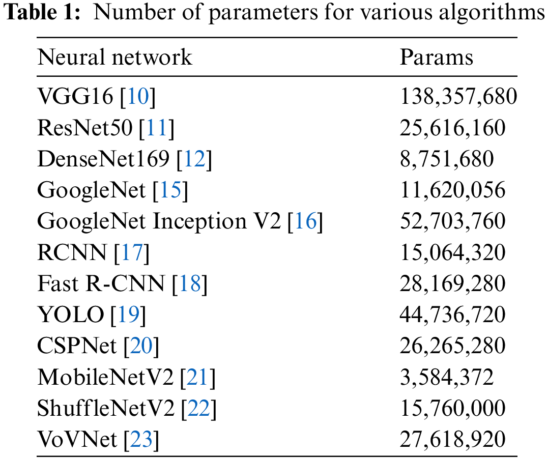
The larger the number of parameters, the greater the arithmetic requirement for the computer, and the stability and accuracy of the results depend largely on the tuning of the parameters. In order to solve the parameter tuning problem, the back propagation algorithm is introduced into the network, which feeds the results back to the neural network, finds the local optimal solution through the derivative, and changes the parameters of the neurons to optimize them, and then reaches the local minimum. When the parameters fall into the local optimal solution, the dropout strategy can intervene by setting some of the neuron parameters to zero during the iteration process, which not only prevents the parameters from being limited by the local optimal solution, but also shifts the initial values of the parameters to new values in order to find a better solution. This suggests that, theoretically, the more the network parameters and the greater the depth of the network, the better the performance should be. However, when backpropagating, a large number of parameters can make it difficult for the gradient to pass through the deep network, limiting the superposition of the network depth and thus triggering overfitting and slowing down the training. To address this problem, several approaches exist to reduce the number of model parameters such as lightweight processing while improving the accuracy of target recognition. The following briefly analyzes the improvement modules of three strategies aimed at solving the overfitting phenomenon as well as improving training efficiency.
2.1 Convolutional Layers Instead of Fully Connected Layers
Convolutional layers and fully connected layers have different roles and advantages in neural networks, and many studies have pointed out the application of convolutional layers in reducing the number of parameters, improving computational efficiency and model generalization ability. The convolutional layer can effectively reduce the number of model parameters and improve computational efficiency through its local connection, sparse connection and weight sharing. On the contrary, fully connected layers rely on the global information of the image and each neuron is connected to all neurons in the previous layer, resulting in a large number of parameters. However, it has been shown that the “maximal local” processing power of convolutional layers is essentially equivalent to the “global” processing power of fully connected layers, which means that in some cases it is possible to use convolutional layers as an alternative to fully connected layers, thus reducing the complexity of the model without sacrificing performance.
For specific applications, Cosmin Duta, Ionut et al. investigated a pyramid shaped neural convolutional structure that 5 can handle input images of different sizes without increasing the computational cost and the number of parameters [24]. In addition, Faster R-CNN enhances the expressiveness and generalization of the model by replacing the traditional selective search method with a region proposal network (RPN) and employing convolutional layers instead of fully connected layers. Similarly, YOLO [19] significantly improved the computational efficiency and accuracy of the model by using a convolutional neural network to implement a single inference on an image and replacing the fully connected layers with convolutional layers, developed a multilayer system model for real-time target detection based on an improved single multi-frame detector algorithm, which effectively improves the performance in the task of target detection by replacing the fully connected layers with convolutional layers. All these works demonstrate the significant advantages of convolutional layers in improving model efficiency, reducing parameters and enhancing performance, corroborating the feasibility and effectiveness of replacing fully-connected layers with convolutional layers in appropriate cases.
2.2 Deeply Separable Convolution Replaces Traditional Convolutional Layers
Deep separable convolutional networks, a convolutional neural network architecture applied in computer vision tasks, achieve the goal of improving network efficiency and accuracy by splitting the conventional convolution operation into two steps: deep convolution and point-by-point convolution. This architecture performs convolution operations on each channel of the input feature map individually through deep convolution, utilizing smaller convolution kernels such as 3 × 3 to effectively reduce the number of parameters and focus on local feature extraction. Subsequently, point-by-point convolution enhances the nonlinear capability of the model by merging information fromdifferent channels.
Recent research results demonstrate the advantages of depth-separable convolution for practical applications. Residual blocks can be used to successfully improve model performance and stability by replacing traditional convolutional layers with depth-separable convolution [11]. ShuffleNet achieves the goal of obtaining high performance while maintaining low computational complexity and number of parameters by replacing traditional convolutional layers with depth-separable convolution and introducing a random ordering operation to improve the nonlinearity of the model [25]. Similarly, SqueezeNet employs deeply separable convolution to replace the traditional convolutional layers and further reduces the number of parameters of the model through a squeezing operation [26].
In addition, the segmentation operation of depth-separable convolution optimizes the gradient flow during backpropagation and effectively mitigates the problems of gradient vanishing and gradient explosion, hence the important role of depth-separable convolution in improving the model training efficiency and performance robustness. Overall, depth-separable convolution, through its innovative structure, not only reduces the number of parameters but also enhances the nonlinear properties of the model, thus playing a key role in various image recognition and computer vision such astracking tasks.
The Densely Connected Networks module, inspired by shortcut connections in residual networks, introduces a method of feature fusion that is different from the direct addition of feature vectors. This approach not only enhances the information content in a particular feature graph, but also increases the dimensionality of the feature graph at each depth level, i.e., it extends both the depth of the feature graph and the dimensionality of the feature vectors. The dense connectivity algorithm model, which adopts the strategy of using the feature maps of all previous layers as inputs to each layer and using the feature maps of the current layer as inputs to all subsequent layers, is designed to not only alleviate the gradient vanishing problem but also enhance the feature propagation, and it significantly reduces the number of parameters of the model [12].
In addition, by introducing a dense connectivity strategy, also known as Dense Connected Graph Convolutional Network (DCGCN), this network is able to integrate local and non-local features to learn the representation of graph structures more efficiently [27]. In summary, the dense connected network effectively reduces the number of parameters while improving the model performance through its innovative feature fusion and parameter optimization strategies, and these advantages have been validated in different research and application scenarios.
3 Lightweight Scale-Adaptive Scaling Models
3.1 Diagram of VGGNet Network Structure and DCDSNet Network Structure
VGGNet extends the number of channels by introducing the concept of combining convolutional layers into blocks, i.e., VGG-blocks, and by not limiting the number of layers and channels of convolutional layers in a block. The design of multiple VGGNet networks is uniform. The difference lies in the design of the intermediate VGG-block blocks. In AlexNet, each layer contains only one convolution with a 7 × 7 convolution kernel. The most noticeable improvement in VGGNet is the reduction in the size of the convolution kernel and the increase in the number of convolution layers.
Using multiple small convolutional kernels instead of a single large convolutional kernel, not only reduces the number of parameters in the model but also increases the number of nonlinear mappings, which improves the network’s ability to adapt and fit.VGGNet goes from an 11-layer A model to a 19-layer E model, and the increase in the depth of the network significantly improves the recognition rates of the top1 and the top5. The structure of the VGG19 network structure is shown in Fig. 1 [10].
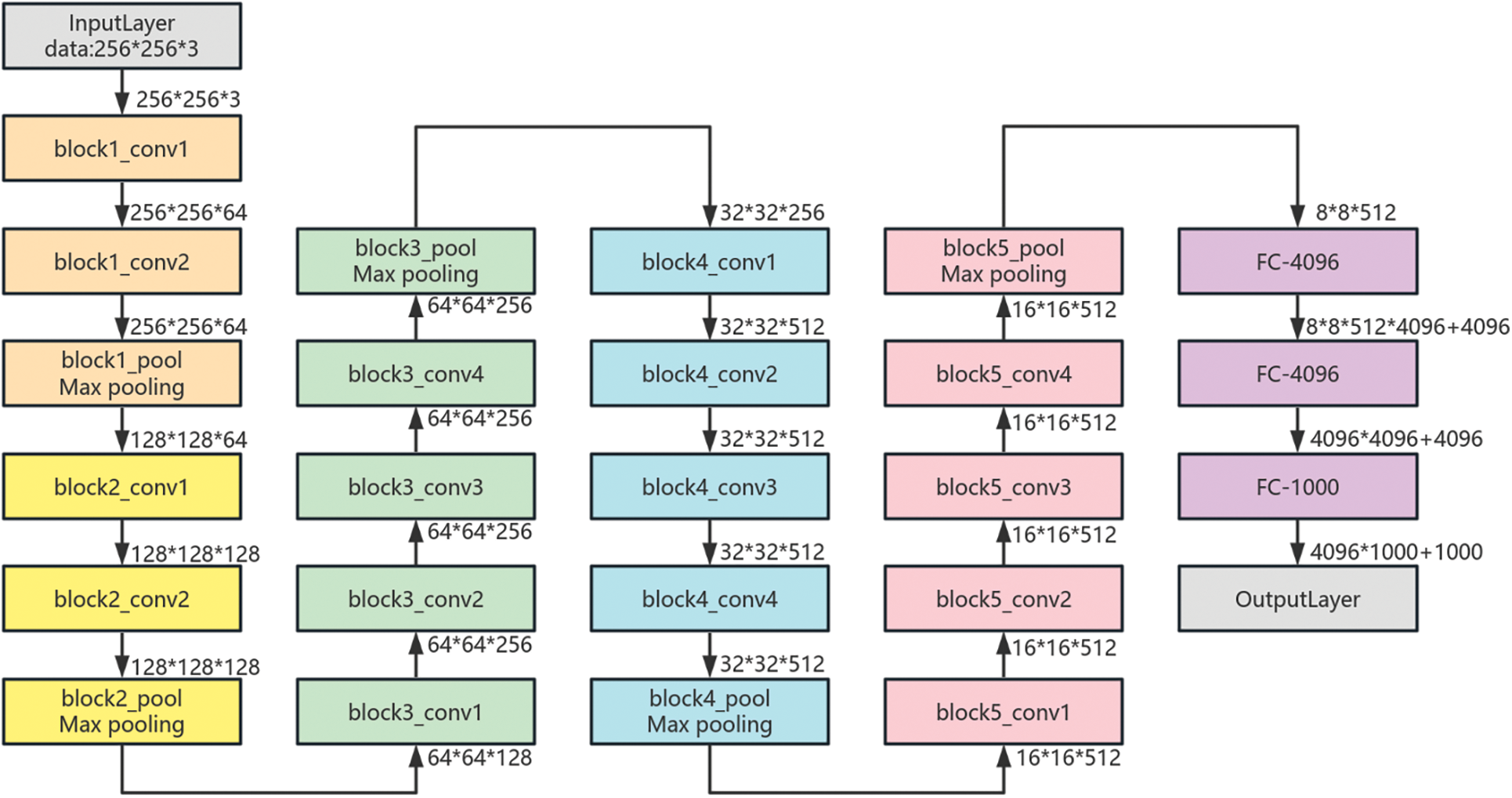
Figure 1: VGG19 network structure diagram
The VGG19 has 16 convolutional layers and consists of five convolutional modules, each of which maintains the same size and depth of the convolutional layers within each module and is connected by a maximum pooling layer. The first module contains two convolutional layers each using 64 3 × 3 convolutional kernels; the output of this module is connected to a maximal pooling layer using a 2 × 2 sliding window and a step size of 2. This configuration is used for the maximal pooling layer throughout the network; the second module similarly consists of two convolutional layers using 128 3 × 3 convolutional kernels; the third module consists of four 3 × 3 convolutional kernels using 256 convolutional layers; the fourth and fifth modules both contain four convolutional layers using 512 3 × 3 convolutional kernels, and the fifth module is followed by a maximum pooling layer and three fully connected layers. The input image is a 3-channel image of 224 × 224 size. Although the VGG19 model has excellent recognition performance, it has a very large number of parameters. The three fully connected layers of this network have a total of 102765544 parameters, which accounts for 71% of the total number of parameters in VGG19. The excessive number of parameters can lead to overfitting and reduce the computational speed.
According to the propagation process of feature maps in the VGG19 model, the length and width of the feature maps are halved for every maximum pooling layer passed, while the depth of the feature maps is increased for every convolutional layer passed. With the increase of layers in the model, the focus on the local information of the original image is gradually reduced, and instead the image features are redistributed in different depth layers, eventually, these feature maps are passed to the fully connected layer. Although the compression function of the fully connected layer has both advantages and disadvantages for the model as a whole, it compresses the feature map into a feature vector, such compression, although helps in data processing, has the disadvantage that it may lead to the loss of local information. It further makes the classification layer insufficient for feature extraction and affects the classification accuracy. The DCDSNet network proposed in this chapter is based on the VGG19 network framework. The overall structure of the DCDSNet network structure is shown in Fig. 2 below.
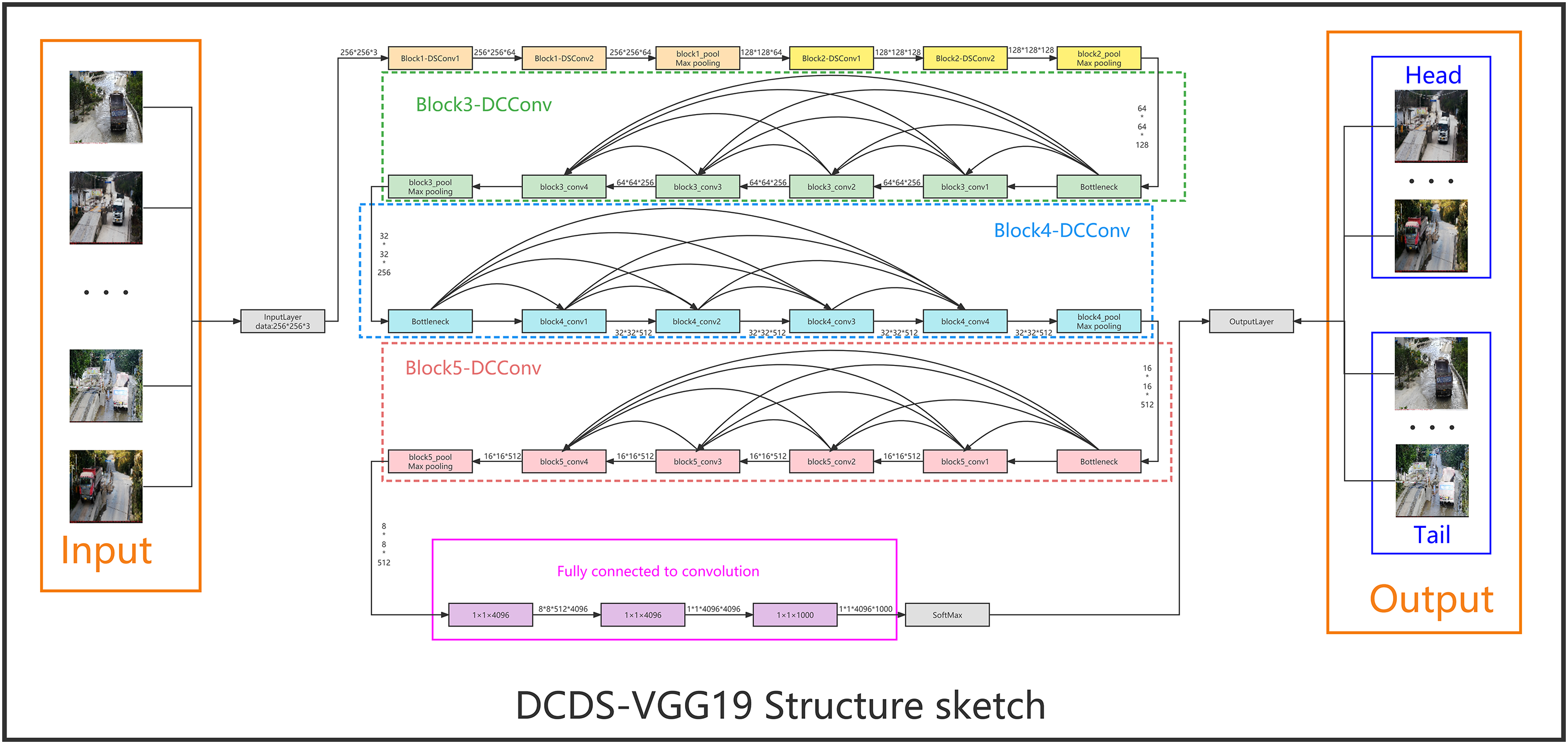
Figure 2: Schematic diagram of DCDSNet network structure framework
The DCDSNet algorithm whose backbone network uses the VGG19 framework greatly reduces the number of network parameters by replacing the last three fully connected layers with 1 × 1 convolutional layers. Depth separable convolution is introduced to replace the original convolution, to solve the limitations of hardware in memory access speed and throughput, and the number of convolution space channels is adjusted by increasing or decreasing the expansion factor, which is actually the convolution kernel, and each convolution kernel corresponds to an output channel, and the so-called channel is a feature map. The model is optimized using a dense connection technique, as shown in Fig. 2 Each stage uses cross-layer connections to input, shallow features into the deeper network modules that follow, enabling the DCDSNet model to extract feature information more comprehensively. The advantages of DCDNet utilizing smaller convolutional kernels are analyzed below, as well as the specific analysis of the DCDSNet network constructed by the three techniques convolution instead of full connectivity, deep separable convolution instead of the original convolution, and dense connectivity.
3.2 Computation and Sensory Fields for Small Convolutional Kernels
DCDSNet uses smaller convolution kernels for reasons such as less computational effort, a small number of parameters, and multi-level accumulation of small convolution kernels with equal receptive fields as large convolution kernels. Convolution involves more than computational effort, it also affects the sense field. Small convolutional kernels are easily deployed for mobile devices, can fulfill real-time processing, and are easy to train and other related. The size convolution kernel involves parameter updates, the size of the feature map, whether enough features are extracted, the complexity of the model, and the number of parameters. In order to highlight the computational advantages of small convolution kernel, the same conv 3 × 3, conv 5 × 5, conv 7 × 7, conv 9 × 9 and conv 11 × 11 are taken and convolved on 224 × 224 × 3 RGB maps, respectively. The parameters of the convolution layers and the size of the resulting feature maps are shown in Table 2 below.
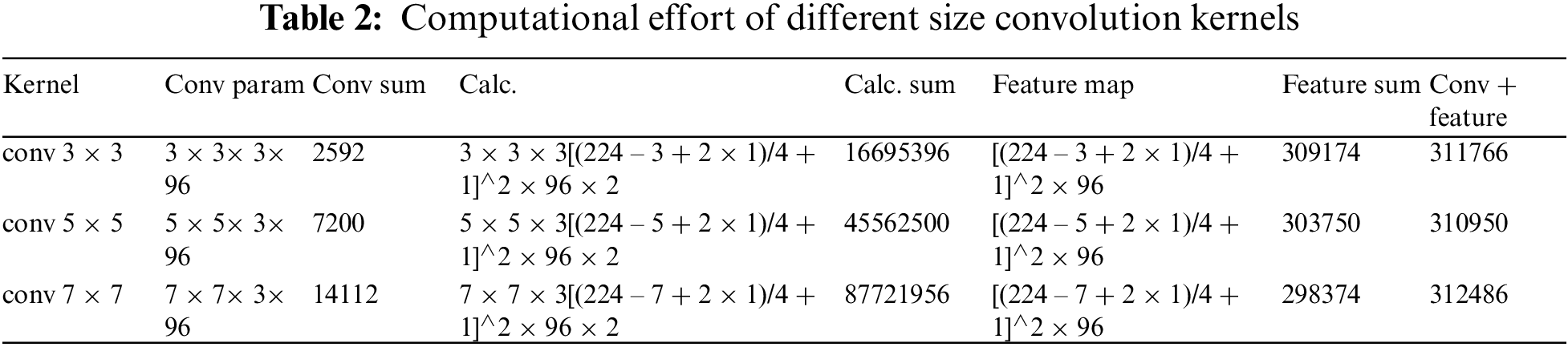
(1) From Table 2, we can see that the number of parameters of the feature map is not much affected by the size of the convolution kernel.
When looking at a single convolution kernel parameter or feature map parameter, the total number of parameters for both structures at different convolution kernel settings is approximately 300,000. However, this structure increases the computational effort of the convolution operation, which is reflected in the formulas listed in the table, where the final multiplication of the formulas by two denotes the multiplication and addition operations. For consistency, the step size here is set to 4. As can be seen from the data, the five different convolutional kernels amount to 16, 45, 140 and 200 million computations, respectively, which is a very large difference in computational volume. As far as the number of parameters is concerned, the convolutional kernel parameters are usually in the 100,000 level and rarely exceed one million. This is due to the fact that the number of parameters is the product of the number of neurons in the upper layer of the feature map and the number of fully connected kernels, as compared to the fully connected layer, thus increasing the computational effort. In addition, the combined use of multiple small convolutional kernels is also a factor. The ability to be smaller compared to a single large convolutional kernel is an important corroboration of the fact that DCDSNet utilizes small convolutional kernels. Also, the number of parameters is reduced.
(2) The sensory field of different convolutional kernels. As shown in Fig. 3, when convolving through three layers of conv 3 × 3 convolution, the elements of the bottom layer inputs can be thought of as the width or height of the feature map when the input neuron is convolved to obtain a neuron, meaning that each element of the bottom layer input corresponds to a neuron in the feature map generated after the convolution operation. These three networks correspond to the convolution kernels conv 3 × 3, conv 5 × 5, and conv 7 × 7 at layers 3, 1, and 1, respectively, with a step size of 1 and a padding of 0. Assuming an input of 7 for all three networks, it can also be seen that the stack of 2-layer 3 × 3 convolutions obtains a receptive field of size equivalent to a 1-layer 5 × 5 convolution, whereas the stack of 3-layer 3 × 3 convolutions obtains a receptive field equivalent to a 7 × 7 convolution. This is shown in Fig. 3.
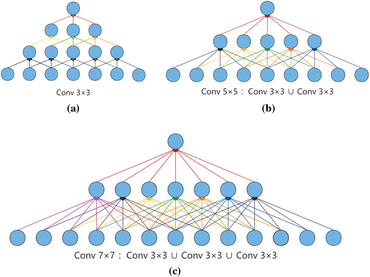
Figure 3: (a), (b) and (c) show the correlation between the three convolutional kernels
Or we can say that a three-layer conv 3 × 3 network with one neuron in the last two outputs sees a receptive field equal to the 3 in the previous layer, the 5 in the layer above it, and the 7 (i.e., the input) in the layer above it. The concept of a receptive field (receptive field) in a convolutional neural network (CNN) and how it expands as the number of layers in the network increases. The receptive field is the range of response of a particular neuron to a localized region of the input image in a CNN. In Fig. 3c, a three-layer convolutional network is depicted, with each layer using a 3 × 3 convolutional kernel.
In this network, it is assumed that we focus on one neuron in the last two outputs. The receptive field of this neuron is described as equal to 3 in the previous layer, 5 in the layer above it, and 7 in the layer above it, which means that in order to compute the output of this neuron, it needs to “perceive” a localized region of 3 × 3 in the previous layer, and each neuron in this localized region needs to perceive a localized region of 5 × 5 in the previous layer, and a localized region of 5 × 5 in the layer above it, as well as a localized region of 5 × 5 in the layer above it. and a 7 × 7 localized region in the previous layer. In other words, the response of this neuron to the input image is transmitted layer by layer through the convolution operation, with each layer expanding the receptive field. This layer-by-layer transfer allows the network to understand the global features of the input image at a higher level, allowing for more complex feature extraction and representation.
The rationalization for using 3 × 3 convolution instead of sensory field is explained by the advantages of using a small convolutional kernel over a large convolutional kernel having more activation functions, richer features and better discrimination. Using more convolutional kernels gives the decision function higher discriminative power, and in terms of the convolution itself, 3 × 3 is sufficient to capture more feature variations than 7 × 7: the nine units of 3 × 3, with the middle unit as the center of the receptive field, capture feature variations in the top, bottom, left, right, and diagonal [28]. The network is two layers deep, with two additional nonlinear ReLU functions, which allows the network to have more capacity and to be more discriminative.
3.3 Convolutional Alternative to Fully Connected
One of the more innovative features of the DCDSNet network structure is the switch from fully connected to convolutional [29], where the original three fully connected layers in the network were changed to one conv 7 × 7 and two conv 1 × 1 convolutional layers during the testing phase. This change left the network missing the fully connected layers. The feature maps in the middle of the network can be of different sizes, thus allowing the network to handle inputs of any size. The fully connected replacement for convolution is shown in Fig. 4.
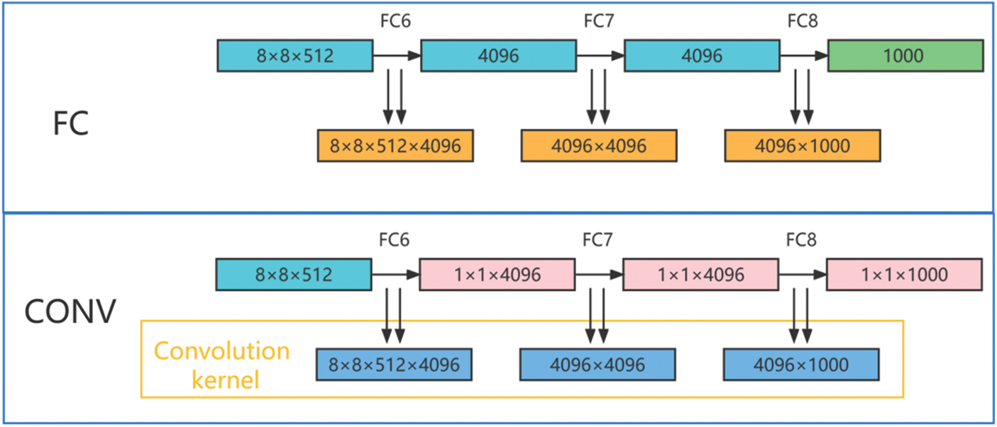
Figure 4: Convolutional alternative to fully connected comparison structure
Fig. 4 shows a comparison of convolution instead of fully connected structure. The top half shows the last three layers of the original VGG network which are fully connected layers their outputs are 4096, 4096, and 1000, respectively, and the bottom half shows the last three layers of the DCDSNet framework, where the last three layers become convolutional layers whose outputs are 1 × 1 × 4096, 1 × 1 × 4096, and 1 × 1 × 1000, respectively. the fully connected layer, FC6, with an output of 4096, receives an 8 × 8 × 512 feature map as input. In the fully connected layer, a total of 32,768 elements of 8 × 8 × 512 can be treated as a whole since there is no need to focus on the localization of the elements. All of these input elements are connected to each element of the output layer, i.e., each input will have 4096 outputs, and the size of the network is 8 × 8 × 512 × 4096. For FC7 with 4096 inputs and outputs, since each input is connected to an output, i.e., each output has 4096 connections, the total of 4096 inputs will have 4096 × 4096 connections, which gives the FC8 a parameter size of 4096 × 1000. In the DCDSNet network, when switching to convolution, the first convolution is used to obtain 4096 outputs, so the width and height of the 8 × 8 × 512 feature map must be reduced and the depth must be boosted. In addition, the 8 × 8 convolution reduces the width and height to 1 × 1 and increases the depth level to 4096, i.e., a 1 × 1 × 4096 feature map is obtained. The second convolution, since the input is also 1 × 1 × 4096, still produces a 1 × 1 × 4096 output, with the three dimensions width, height, and depth unchanged, so the size of the convolution kernel for this layer can be computed to be 1 × 1 as well, and the number of channels is also 4096. The convolution parameter for all 4096 outputs is then considered to have a size of (1 × 1 × 4096) × 4096. The third convolution is similarly computed as (1 × 1 × 4096) × 1000. Theoretically referencing the work of OverFeat [30], which can handle convolutional computations of arbitrary resolution without resizing the original image. The most obvious difference between convolution and fully-connected is the local connection, but both use global information, except that convolution utilizes it by stacking layers on top of each other. Fully-connected directly uses all the feature maps from the previous layer, with greater sparsity, whereas convolution obtains global information by increasing the depth of the network, layer by layer, based on the input from the current layer.
3.4 Introducing Deeply Separable Convolution
The original VGG took a long time to train the model due to the large number of parameters in the model, so the first two layers of convolution of the convolution block were replaced with depth separable convolution in the DCDSNet framework and the improved module was named Block-DSConv. The structure of the model is shown below in Fig. 5.
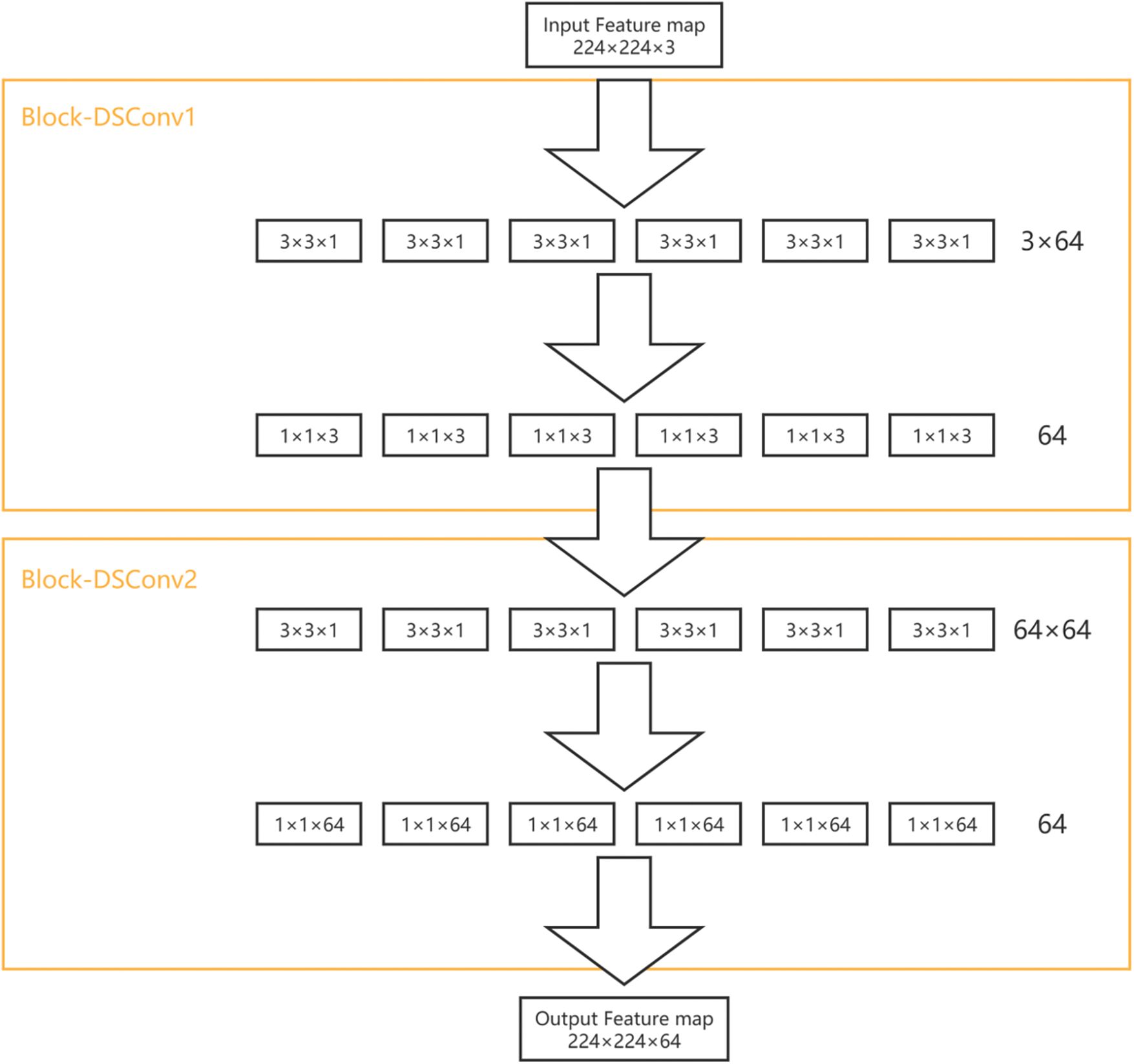
Figure 5: Block-DSConv structure diagram
(1) Comparison and calculation of the number of depth-separable convolutions compared to the original convolutional parameters. As can be seen in Fig. 5, the size of the resulting feature map is the same as that obtained for the original network. However, there is a significant difference between the two in terms of the number of parameters. Imagine that the input feature map has a given dimension such as
The depth separable convolution is calculated as shown in Eq. (2). Eq. (3) gives the relationship between the number of depth separable convolution parameters and the number of standard convolution parameters.
(2) As shown in Fig. 6, the comparison between depthwise separable convolution and traditional convolution is shown, and the parameter quantities of depthwise separable convolution and traditional convolution are calculated separately. If the size of the input feature map is 224 × 224 × 3, the first convolution module of the VGG19 model contains two convolutional layers, each containing 64 convolutional kernels. Among them, the first layer has 3 × 3 × 3 convolution kernels and the second layer has 3 × 3 × 64 convolution kernels, and each convolution layer is divided into channel-by-channel and point-by-point convolution. For example, in the first layer, a 3 × 3 × 3 convolution kernel is split into three separate convolution kernels of 3 × 3 size and 1 depth. In the second layer, a large convolutional kernel is then split into 64 smaller convolutional kernels. After using the depth-separable convolution technique, the size of the input feature map is maintained as 224 × 224 × 3. The size of the output feature map is 224 × 224 × 64. The number of parameters for the depth-separable convolution is 3 × 3 × 3 + 3 × 64 + 3 × 3 × 64 + 64 × 64 = 4891, whereas the sum of the number of parameters for the two convolution layers of the original network is 3 × 3 × 3 × 64 + 3 × 3 × 64 = 38,592. 64 × 64 = 38,592. the number of parameters is reduced by 87.33%, but the accuracy of the model is 90.35% for the same number of iterations, showing that the reduction of parameters also reduces the performance of the model. In order to solve this phenomenon, therefore the dense connectivity technique was introduced in DCDSNet to further improve the accuracy of the network.
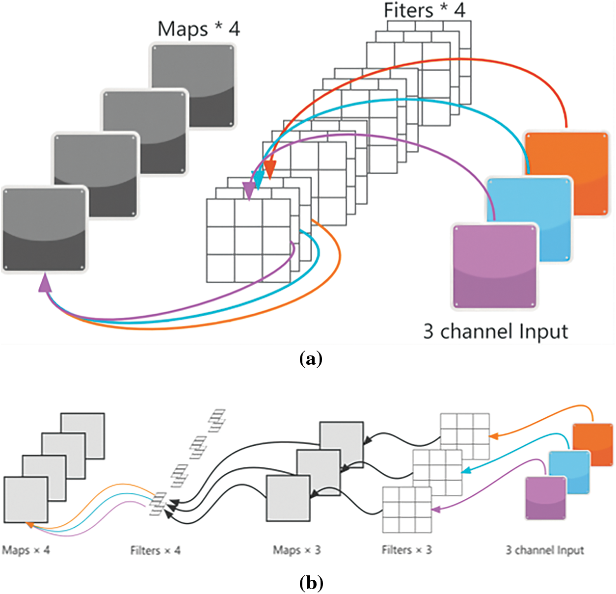
Figure 6: The upper a figure represents the conventional convolutional computation process, and the lower b figure represents the depth-separable convolutional computation process (Reprinted from Reference [17])
(3) Depth separable convolution is a convolution operation for extracting feature maps that combines deep convolution (DW) and pointwise convolution (PW) components. Compared to conventional convolution operations, deep separable convolution has a lower number of parameters and computational cost. However, deep convolutions are relatively computationally inefficient because they require a large number of data transfers compared to the number of floating-point operations performed, which means that the speed of memory access is a critical factor. Although there may be throughput limitations on alternative hardware, the memory architecture in the processor provides high bandwidth memory accesses that can significantly improve the performance of such computationally less efficient operations. Experimental data suggests that deep convolutions are most efficient when placed in MBConv blocks formed between two pointwise “projected” convolutions. These pointwise convolutions increase or decrease the dimensionality of the activations by adjusting the “expansion factor”, or convolution kernel, around the spatial depth convolution. While this expansion can lead to good task performance, it also creates a very large activation tensor that can dominate memory requirements and ultimately limit the maximum batch size that can be used.
In deep convolution (DW), each channel is processed by a separate convolutional kernel, ensuring that each channel is only affected by its corresponding convolutional kernel. This approach ensures that the number of feature maps in the output is exactly the same as the number of channels in the input. For example, when performing deep convolution on a three-channel 5 × 5 pixel color input image, the convolution is performed entirely in the two-dimensional plane, with each channel performed independently, resulting in three feature maps. The core of deep convolution is that it has the same number of convolution kernels as the number of channels in the input layer, generates one feature map per channel, and does not increase the number of feature maps. Furthermore, this operation processes each input channel independently and does not integrate information from different channels at the same location. Therefore, it is often necessary to combine these independent feature maps by punctuated convolution to create new feature maps.
The process of pointwise convolution (PW) is very similar to standard convolution in that it uses a convolution kernel of dimension 1 × 1 × M, where M represents the number of channels in the previous layer. The dimension of the convolution kernel is 1 × 1 × number of input channels×number of output channels. The feature of using 1 × 1 convolution is that the number of relevant convolution parameters can be computed, e.g., 1 × 1 × 3 × 4 = 12 for N_pointwise and 1 × 1 × 3 × 3 × 3 × 3 × 4 = 108 for C_pointwise. After performing pointwise convolution, the output is still a 4-feature map, which is of the same dimensions as those generated by regular convolution.
3.5 Densely Connected Network Modules
Theoretically, increasing network parameters and depth can improve network performance. However, in practice, these factors may lead to problems such as gradient vanishing or gradient explosion, which limit the depth and performance of the network. The backbone network of the DCDSNet model proposed in this chapter is chosen to be the VGG19 model, which is the deepest and most parameterized of the VGG networks, although it does not perform particularly well in current vehicle tracking networks, and in order to improve the tracking accuracy, the developers have used the dense connection technique to optimize the model. This improvement allows the DCDSNet model to extract feature information more efficiently, which enhances tracking accuracy on relevant datasets. The improved convolutional block is named Block-DCConv, a densely connected convolutional module. In densely connected networks, the dimension of the feature maps for each layer of the same convolutional module needs to be consistent. DCDSNet contains five convolutional modules with the same structure and feature map depth, which makes it particularly suitable for applying densely connected techniques [31]. The structure of Block-DCConv1 is shown in Fig. 7.
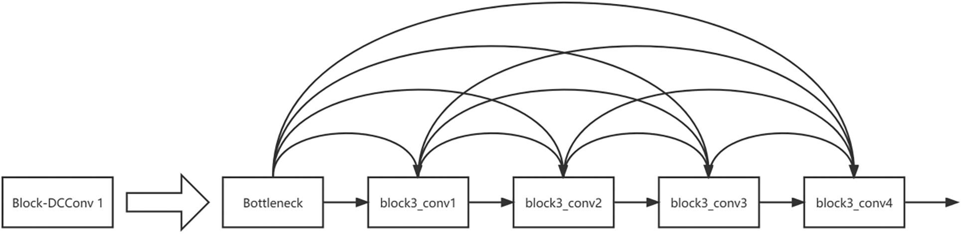
Figure 7: Schematic structure of Block-DCConv1 densely connected convolutional module
Block3_conv1 is a convolutional layer with 32 convolutional kernels of size 3 × 3, which is a reduction in the number of convolutional kernels compared to the 256 convolutional kernels of the same size in the original convolutional module. This adjustment is due to the rapid expansion of the number of channels in the feature map after Block-DCConv. The following equations demonstrate this change:
where
A bottleneck structure was added to Block-DCConv [32]. The bottleneck is a 1 × 1 point convolution, which also aims to reduce the dimension of the feature map and has the effect of reducing the number of parameters. The dimension of the feature map of the input layer is 128 × 56 × 56. Without the bottleneck structure, the parameters are 3 × 3 × 32 × 128 = 36,864, whereas with the addition of the bottleneck structure, the number of parameters is 3 × 3 × 32 × 64 + 1 × 1 × 64 × 128 = 26,624, which reduces the number of parameters by 10,240 for each convolutional layer.
In our experiments, we found that compared to VGG19, DCDSNet despite the reduction in the number of parameters, this leads to higher memory usage. The feature maps need to allocate new space in the graphics memory to store the fused feature maps during multiple fusions. Each convolutional module is stored in the format (3–i+1) and contains three Block-DCConv units, which in practice makes the memory consumption equivalent to the memory requirement of a six-layerconventional network.
4.1 Data Set Composition and Design Ideas
In this chapter, the proposed DCDSNet network is used to recognize and track mining trucks, there are 12,211 data images, including 4073 pictures of the front end and 4065 pictures of the rear end, and 7789 pictures of special vehicles that cannot be tracked by the original system, and this dataset is named as Truck-20000. the images are turned into video streams to complete the tracking, and statistics of tracking accuracy are provided. The first step is to divide the dataset with Python code, divide the dataset into training set and test set, and save them in the target folder respectively. The ratio of training set and test set is set to 3:2 for training and testing, respectively. The second step is to download the VGG19 model, tune through it and construct the DCDSNet model algorithm proposed in this chapter according to the three techniques, train the divided data to obtain the training model, and then test the data using the trained model to obtain the test results to realize the recognition and tracking of the mine carts. Fig. 8 shows the distribution of the number of images in the training and test sets in the dataset.
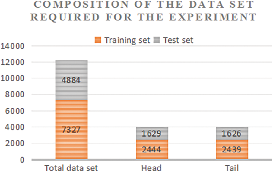
Figure 8: Division of dataset training set and test set
4.2 Development Environment and Network Parameters
The platform is based on the Python language and is developed using PyCharm version is 2020.3.3 ×64 and Anaconda3 as the development tool for the platform. Anaconda comes with many common third-party libraries such as Python and Anaconda Prompt.Torch is a third-party library for Python used in large-scale machine learning applications. It is well suited for image and video recognition and tracking.Torchvision can be used primarily to load images and perform simple operations on them. The experimental training environment is displayed in Table 3.
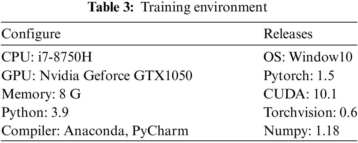
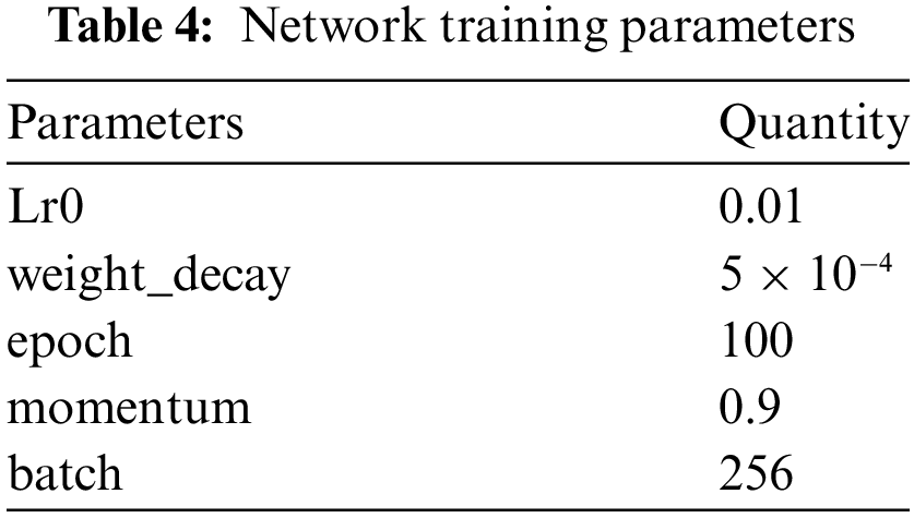
Table 4 shows the parameter configurations used in the experiments for network training. In supervised and deep learning, the learning rate Ir0 is a hyperparameter that can affect whether the objective function and its convergence time can reach a local minimum. A higher learning rate can speed up the learning of the network in the early stages of training and help the model approach the optimal solution faster. However, this can lead to larger fluctuations in the later stages, even causing the loss function value to fluctuate near the minimum, with large fluctuations and always difficult to reach the optimum, so the scheme used in this chapter is to use small batch gradient descent with the following parameters: the batch size is set to 256, and the momentum is set to 0.9. Momentum is a common technique used in the gradient descent method to accelerate convergence. The initial rate of learning was set to 0.01 and the decay coefficient of the weights was 5 × 10⁻⁴. For the weights layer, a stochastic initialization was used, initialized to a normal distribution with a mean of 0 and variance of 0.01. The width and height of the mining truck image data is 1920 and 1080, respectively, which is not suitable for training, so the data needs to be preprocessed to a width and height of 224. the name of the model used is DCDSNet.
In data preprocessing, we resize the image to 224 × 224, which meets the input requirements of the DCDSNet network, save the organized image set under the data file, pass the number of local data batches to be trained as a parameter, set the corresponding parameter mean = [0.5, 0.5, 0.5], variance std = [0.5, 0.5, 0.5] and then normalized. In the experiment, the image is first read and then resized to the specified size. After preparing the data import process, the training and test sets need to be sliced and diced, and the experiment involved in this paper slices the mining truck dataset according to the ratio of 3:2. For the training and test sets, the corresponding image data indexes need to be made first, i.e., two files train.txt and test.txt, respectively, each txt contains the directory of each image and the corresponding category. The weights and bias coefficients to be learned during the training process are stored through the defined training model train_model and the parameter best_model_wts, and the return values are received using the variable data structure commonly used in neural networks. After 100 training cycles, the training results obtained at the VGG19 model are shown in Fig. 9.
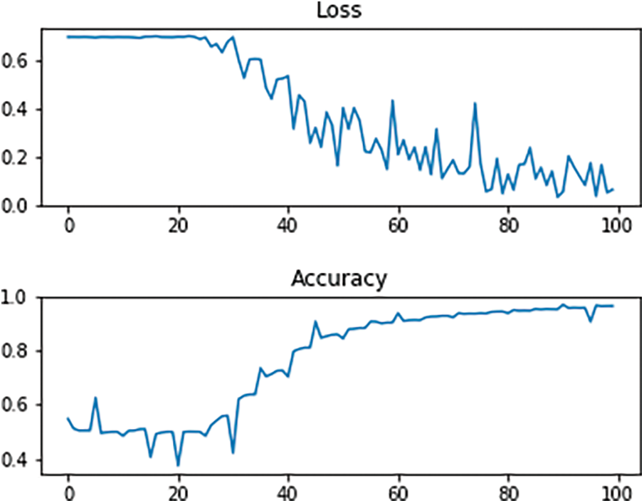
Figure 9: Training loss and accuracy change curves on VGG19 for 100 iterations
4.4 DCDSNet Network Test and Experimental Results Analysis
In our experiments, we will keep the best model and set the learning rate for the import dynamics. First, we generate a random image of size 224 × 224 and generate normally distributed random numbers with a standard deviation of 0.1 via the tf.random_normal function. Next, a placeholder for keep_prob is created and the inference_op function is called to construct the network structure of DCDSNet, obtaining the prediction, softmax, fc8, and the parameter list p, creating the session, and initializing the global parameters. The time consumption of DCDSNet in tensorflow is tested by executing the main function run_benchmark() of the evaluation. The results are retained and images are generated to output the Loss and Acc. For the accuracy of the experiments, we adjust the accuracy of the original ten cycles containing the training set as well as the test set, with batch_size set to 32 and epochs to 20 in Experiment 1, batch_size set to 32 and epochs to 30 in Experiment 2, batch_size set to 32 and epochs to 30 in Experiment 3, and batch_size set to 32 and epochs to 30 in Experiment 3. size is set to 32 and epochs to 100 and the output is shown in Fig. 10.
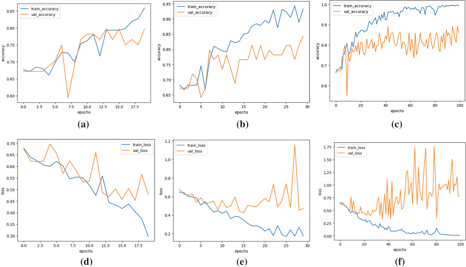
Figure 10: Curves of Acc, Loss of DCDSNet test model with increasing number of trainings, (a), (d) correspond to the change curves of Accuracy and Loss for 20 iterations of the algorithm in Experiment 1. (b), (e) correspond to the change curves of Accuracy and Loss for 30 iteration of the algorithm in Experiment 2. And (c), (f) correspond to the change curves of Accuracy and Loss for 100 iterations of the algorithm in Experiment 3
Fig. 10 represents the Accuracy and Loss changes of the DCDSNet model for three different experiments. Experiment 1 has 20 iterations, Experiment 2 has 30 iterations, and Experiment 3 has 100 iterations. Fig. 10a–c plots represent the three experiments Accuracy change curves gradually converge to about 0.95 with the increase of the number of training times, respectively. Fig. 10d–f plots represent the three experiments Loss change curves gradually converge to about 0.02 with the increase of the number of training times, respectively. the return value will be received, the value with the highest probability is taken, setting the gradient to zero, obtaining the loss and then calculating the loss to return, and then updating the parameters. The values obtained will be counted. The results are displayed in Table 5.
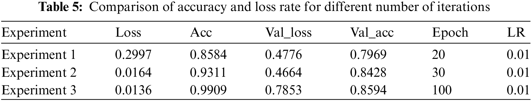
It is obvious from the results that the improved model has a significant improvement in accuracy compared to the unimproved VGG algorithm model, with the maximum value of Acc reaching 99.09% after training. In order to better analyze the values of the experimental results, we counted the results such as the accuracy of the front-end vehicle recognition experiments and the average accuracy of the recall tracking in the three experiments, and the results are displayed in Table 6.
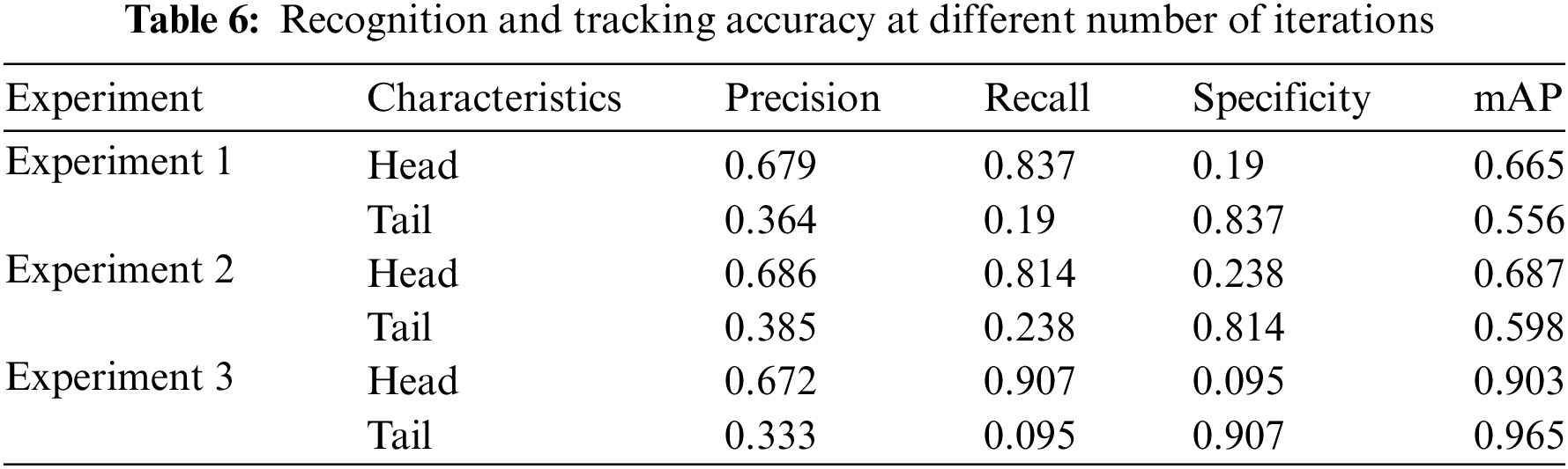
In Table 6, Accuracy measures how many of the results predicted by the binary classifier as positive instances are correct from a prediction point of view. Recall, on the other hand, evaluates the proportion of actual positive examples in the test set that were correctly recognized by the biclassifier, from the perspective of real results. Specificity is the proportion of true negative examples that the model is able to detect. mAP represents the average accuracy of the tracking, which increases with the number of iterations. In the experiments there is a significant improvement in the accuracy of the system as the training cycles are stacked.
4.5 Experiments with Mine Car Data
The traditional deep convolutional neural network based head and tail recognition system experiments use 16,000 images for training and 4000 head and tail for testing, and the experimental results show that the training accuracy curves are basically converged, and then we use the EfficientNet algorithm based head and tail recognition method to shorten the high-dimensional channels by changing the residual edges of the inverse residual module, introducing a deeply separable convolutional neural network and agent-normalized activation in the moving flip convolution module to offset the non-normalized sources of X- and Y-axis in different dimensions between each convolutional layer, and then improve the model detection rate, and the experimental results show that our network maintains a high accuracy while significantly reducing the Loss value, and the number of parameters is small, and the specific training parameters of the network and the analysis of the results are shown in Table 7.
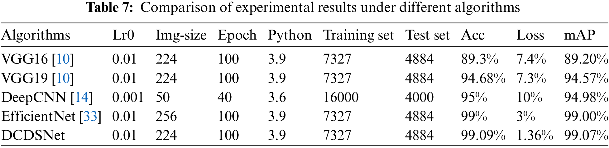
As can be seen from Table 7, for the sake of experimental reliability, we use the same homemade training set as well as the test set, and under the same experimental environment, the accuracy rate of DCDSNet is as high as 99.09%, and the tracking accuracy is 99.0%, which achieves a relatively high recognition accuracy and tracking average accuracy compared with the mainstream model, EfficientNet, and basically meets the mining environment’s basically meets the basic needs of mine car head and tail recognition and tracking in the mining environment.
To ensure what effect the different improvement methods would have on the VGG19 model, we decompose it into multiple models and experimentally validate each model so that the contribution of each module to the accuracy can be clarified in subsequent studies. The DSCVGG model is the model after improving the first two convolutional blocks of the VGG19 using only the deeply separable convolution, the DCCVGG model is the model after improving the first two convolutional blocks of the VGG19 using only the densely connected model after improving the first two convolutional blocks of VGG19, and the DCDSNet model combines all the improved methods. The basic experimental parameter settings as well as the results are shown in Table 8.
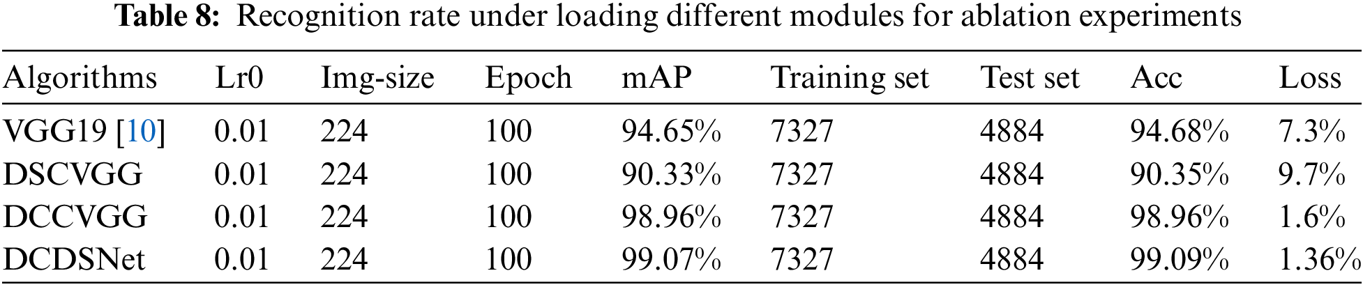
From the table, it can be seen that the DSCVGG model has a 4.33% decrease in accuracy for the same number of iterations as compared to the original network, which shows that the model’s performance decreases while using deeply separable convolution to reduce the parameters significantly. DCCVGG has a 4.28% increase in accuracy over the initial VGG19, which shows that the dense connectivity contributes to the improvement in accuracy. DCDSNet combines the two improved algorithms, which reduces the model parameters while ensuring the performance of the model, improving the performance by 4.41% compared to the original network. The average accuracy of the tracking shows a similar change.
In this paper, we propose a new network, DCDSNet, from real engineering practice, which mainly solves the problem of tracking and recognizing vehicles in the mining environment. The model combines densely connected networks, deeply separable convolution and convolutional alternatives to fully connect to optimize the infrastructure, and the effectiveness of the model is verified in experiments. Through the ablation experiments, it can be found that deep separable convolution can reduce the number of parameters significantly but at the expense of the model accuracy, but combining it with dense connectivity will improve the accuracy of the model significantly. Therefore, one can try to use the dense connectivity method in more models to improve the model performance. The algorithm was applied in the mining environment of mines to track vehicles achieved, better results than the earlier algorithms, according to the feedback of the cooperating companies, the missed recognition rate decreased by 30%. In addition, there are many unfavorable factors for vehicle recognition detection and tracking in the mining environment of mines, such as nighttime, dust, car wash, bad weather and other factors mentioned in the introduction. The dataset used in this algorithm contains images under these factors in achieving this current recognition rate, which helps companies to reduce the workload of manual guards. Further, with the emergence of newer technologies and algorithms, we strive to develop better detection, tracking, and recognition algorithms to meet the requirements of unattended intelligent monitoring systems for mining vehicles in real production scenarios.
Acknowledgement: We sincerely thank the School of Informatics and Engineering of Suzhou University for providing data and experimental equipment to support for this experiment. Special thanks to the teachers of Suzhou University for their coordinated guidance on the overall experiment implementation and deployment in the mine monitoring system process. Special thanks go to the faculty members of Suzhou Vocational College of Civil Aviation, Suzhou University, Tongji University, and Anhui University, whose expertise and insights played a key role in the research of this project. We would also like to thank the Suzhou University for providing the necessary financial to support that greatly facilitated our work. Finally, we would like to thank the contributing team members, colleagues, and participating students.
Funding Statement: This work was supported by the open project of National Local Joint Engineering Research Center for Agro-Ecological Big Data Analysis and Application Technology, “Adaptive Agricultural Machinery Motion Detection and Recognition in Natural Scenes”, AE202210. By the school-level key discipline of Suzhou University in China with No. 2019xjzdxk1. 2022 Anhui Province College Research Program Project of the Suzhou Vocational College of Civil Aviation, No. 2022AH053155.
Author Contributions: The authors confirm contribution to the paper as follows: study conception and design: Chao Wang, Kaijie Zhang; data collection: Dejun Li, Wei Xie, Xinqiao Wang, Xiaoyong Yu, Chao Wang, Kaijie Zhang; analysis and interpretation of results: Chao Wang, Kaijie Zhang; draft manuscript preparation: Kaijie Zhang, Chao Wang. All authors reviewed the results and approved the final version of the manuscript.
Availability of Data and Materials: The data that support the findings of this study are available from the corresponding author, Kaijie Zhang, upon reasonable request.
Ethics Approval: Not applicable.
Conflicts of Interest: The authors declare that they have no conflicts of interest to report regarding the present study.
References
1. N. O. Alsrehin, A. F. Klaib, and A. Magableh, “Intelligent transportation and control systems using data mining and machine learning techniques: A comprehensive study,” IEEE Access, vol. 7, pp. 49830–49857, Apr. 2019. doi: 10.1109/ACCESS.2019.2909114. [Google Scholar] [CrossRef]
2. J. Zhang, F. -Y. Wang, K. Wang, W. -H. Lin, X. Xu and C. Chen, “Data-driven intelligent transportation systems: A survey,” IEEE Trans. Intell. Transp. Syst., vol. 12, no. 4, pp. 1624–1639, Dec. 2011. doi: 10.1109/TITS.2011.2158001. [Google Scholar] [CrossRef]
3. Y. Lin, P. Wang, and M. Ma, “Intelligent transportation system(ITS): Concept, challenge and opportunity,” in IEEE 3rd Int. Conf. Big Data Secur. on Cloud (BigDataSecurity), IEEE Int. Conf. High Perform. and Smart Comput. (HPSC), and IEEE Int. Conf. Intell. Data and Secur. (IDS), Beijing, China, 2017, pp. 167–172. [Google Scholar]
4. L. Qi, “Research on intelligent transportation system technologies and applications,” in 2008 Workshop on Power Elect. Intell. Trans. Syst., Guangzhou, China, 2008, pp. 529–531. [Google Scholar]
5. R. Suryadithia, M. Faisal, A. S. Putra, and N. Aisyah, “Technological developments in the intelligent transportation system (ITS),” Int. J. Sci., Technol. & Manag., vol. 2, no. 3, pp. 837–843, May 2021. [Google Scholar]
6. M. A. Hannan, A. M. Mustapha, A. Hussain, and H. Basri, “Intelligent bus monitoring and management system,” Proc. World Congress on Eng. and Comput. Sci., vol. 2, pp. 24–26, Oct. 2012. [Google Scholar]
7. K. Zhang et al., “Research on mine vehicle tracking and detection technology based on YOLOv5,” Syst. Sci. & Control Eng., vol. 10, no. 1, pp. 347–366, Dec. 2022. doi: 10.1080/21642583.2022.2057370. [Google Scholar] [CrossRef]
8. A. Krizhevsky, I. Sutskever, and G. E. Hinton, “ImageNet classification with deep convolutional neural networks,” Commun. ACM, vol. 60, no. 6, pp. 84–90, May 2017. doi: 10.1145/3065386. [Google Scholar] [CrossRef]
9. M. D. Zeiler and R. Fergus, “Visualizing and understanding convolutional networks,” in Comput. Vis.–ECCV 2014: 13th European Conf., Zurich, Switzerland, Springer International Publishing, 2014,pp. 818–833. [Google Scholar]
10. K. Simonyan and A. Zisserman, “Very deep convolutional networks for large-scale image recognition,” Sep. 2014, arxiv:1409.1556. [Google Scholar]
11. K. He, X. Zhang, S. Ren, and J. Sun, “Deep residual learning for image recognition,” in 2016 IEEE Conf. Comput. Vis. and Pattern Recognit. (CVPR), Las Vegas, NV, USA, 2016, pp. 770–778. [Google Scholar]
12. G. Huang, Z. Liu, L. Van Der Maaten, and K. Q. Weinberger, “Densely connected convolutional networks,” in 2017 IEEE Conf. Comput. Vis. and Pattern Recognit. (CVPR), Honolulu, HI, USA, 2017, pp. 2261–2269. [Google Scholar]
13. A. G. Howard et al., “MobileNets: Efficient convolutional neural networks for mobile vision applications,” Apr. 2017, arxiv:1704.04861. [Google Scholar]
14. J. Li et al., “Deep convolution neural network based research on recognition of mine vehicle head and tail,” in Intell. Comput. Theories and Appl.: 17th Int. Conf., Shenzhen, China, Springer International Publishing, 2021, pp. 594–605. [Google Scholar]
15. C. Szegedy et al., “Going deeper with convolutions,” in 2015 IEEE Conf. Comput. Vis. and Pattern Recognit. (CVPR), Boston, MA, USA, 2015, pp. 1–9. [Google Scholar]
16. C. Szegedy, V. Vanhoucke, S. Ioffe, J. Shlens, and Z. Wojna, “Rethinking the inception architecture for computer vision,” in 2016 IEEE Conf. Comput. Vis. and Pattern Recognit. (CVPR), Las Vegas, NV, USA, 2016, pp. 2818–2826. [Google Scholar]
17. R. Girshick, J. Donahue, T. Darrell, and J. Malik, “Rich feature hierarchies for accurate object detection and semantic segmentation,” in 2014 IEEE Conf. Comput. Vis. and Pattern Recognit., Columbus, OH, USA, 2014, pp. 580–587. [Google Scholar]
18. R. Girshick, “Fast R-CNN,” in IEEE Int. Conf. Comput. Vis. (ICCV), Santiago, Chile, 2015, pp. 1440–1448 doi: 10.1109/ICCV.2015.169. [Google Scholar] [CrossRef]
19. J. Redmon, S. Divvala, R. Girshick, and A. Farhadi, “You only look once: Unified, real-time object detection,” in 2016 IEEE Conf. Comput. Vis. and Pattern Recognit. (CVPR), Las Vegas, NV, USA, 2016, pp. 779–788. [Google Scholar]
20. C. -Y. Wang, H. -Y. Mark Liao, Y. -H. Wu, P. -Y. Chen, J. -W. Hsieh and I. -H. Yeh, “CSPNet: A new backbone that can enhance learning capability of CNN,” in 2020 IEEE/CVF Conf. Comput. Vis. and Pattern Recognit. Workshops (CVPRW), Seattle, WA, USA, 2020, pp. 1571–1580. [Google Scholar]
21. M. Sandler, A. Howard, M. Zhu, A. Zhmoginov, and L. C. Chen, “MobileNetV2: Inverted residuals and linear bottlenecks,” in 2018 IEEE/CVF Conf. Comput. Vis. and Pattern Recognit., Salt Lake City, UT, USA, 2018, pp. 4510–4520. [Google Scholar]
22. N. Ma, X. Zhang, H. T. Zheng, and J. Sun, “ShuffleNet v2: Practical guidelines for efficient cnn architecture design,” in Proc. European Conf. Comput. Vis. (ECCV), Munich, Germany, 2018, pp. 116–131. [Google Scholar]
23. Y. Lee and J. Park, “CenterMask: Real-time anchor-free instance segmentation,” in 2020 IEEE/CVF Conf. Comput. Vis. Pattern Recognit. (CVPR), Seattle, WA, USA, 2020, pp. 13903–13912. [Google Scholar]
24. S. Ren, K. He, R. Girshick, and J. Sun, “Faster R-CNN: Towards real-time object detection with region proposal networks,” IEEE Trans. Pattern Anal. Mach. Intell., vol. 39, no. 6, pp. 1137–1149, Jun. 2016. doi: 10.1109/TPAMI.2016.2577031. [Google Scholar] [PubMed] [CrossRef]
25. X. Zhang, X. Zhou, M. Lin, and J. Sun, “ShuffleNet: An extremely efficient convolutional neural network for mobile devices,” in 2018 IEEE/CVF Conf. Comput. Vis. and Pattern Recognit., Salt Lake City, UT, USA, 2018, pp. 6848–6856. [Google Scholar]
26. F. N. Iandola, S. Han, MW. Moskewicz, K. Ashraf, WJ. Dally and K. Keutzer, “SqueezeNet: AlexNet-level accuracy with 50x fewer parameters and <0.5 MB model size,” Feb. 2016, arxiv:1602.07360. [Google Scholar]
27. Z. Guo, Y. Zhang, Z. Teng, and W. Lu, “Densely connected graph convolutional networks for graph-to-sequence learning,” Transact. Assoc. Computat. Linguist., vol. 7, no. 2, pp. 297–312, Jun. 2019. doi: 10.1162/tacl_a_00269. [Google Scholar] [CrossRef]
28. S. Albawi, T. A. Mohammed, and S. Al-Zawi, “Understanding of a convolutional neural network,” in 2017 Int. Conf. on Eng. and Technol. (ICET), Antalya, Turkey, 2017, pp. 1–6. [Google Scholar]
29. L-C. Chen, G. Papandreou, I. Kokkinos, K. Murphy, and A. L. Yuille, “DeepLab: Semantic image segmentation with deep convolutional nets, atrous convolution, and fully connected CRFs,” IEEE Trans. Pattern Anal. Mach. Intell., vol. 40, no. 4, pp. 834–848, Apr. 2018. doi: 10.1109/TPAMI.2017.2699184. [Google Scholar] [PubMed] [CrossRef]
30. P. Sermanet, D. Eigen, X. Zhang, M. Mathieu, R. Fergus and Y. LeCun, “Integrated recognition, localization and detection using convolutional networks,” Dec. 2013, arxiv:1312.6229. [Google Scholar]
31. Z. Y. Khan and Z. Niu, “CNN with depthwise separable convolutions and combined kernels for rating prediction,” Expert. Syst. Appl., vol. 170, no. 5, May 2021, Art. no. 114528. doi: 10.1016/j.eswa.2020.114528. [Google Scholar] [CrossRef]
32. B. Cui, X. Chen, and Y. Lu, “Semantic segmentation of remote sensing images using transfer learning and deep convolutional neural network with dense connection,” IEEE Access, vol. 8, pp. 116744–116755, Jun. 2020. doi: 10.1109/ACCESS.2020.3003914. [Google Scholar] [CrossRef]
33. C. Wang, K. Zhang, X. Yu, X. Xiong, and A. Zheng, “Lightweight and scale adaptive efficient backbone network for recognition,” Baltica J., vol. 36, no. 7, pp. 2–39, Jul. 2023. [Google Scholar]
Cite This Article
 Copyright © 2024 The Author(s). Published by Tech Science Press.
This work is licensed under a Creative Commons Attribution 4.0 International License , which permits unrestricted use, distribution, and reproduction in any medium, provided the original work is properly cited.
 Downloads
 Citation Tools