Unsupervised Time Series Segmentation: A Survey on Recent Advances

1  Introduction

In recent years, data-driven services, e.g., autonomous driving, and IoT applications, e.g., wearable sensing, have become an indispensable part of daily life, constantly generating a large amount of time series data, a.k.a., KPI (Key Performance Indicator) in AIOps (Artificial Intelligence for IT Operations) domain. These co-evolving multivariate time series time series carry rich information capturing different behaviors and facets of the monitored objects. Exploiting these latent states by segmenting time series could be beneficial for many real-world tasks, e.g., pattern recognition, and event detection [1–5]. Once these patterns are discovered, seemingly complicated time series can be summarized into a compact state sequence, facilitating the highlight elaboration on massive data and many downstream tasks.

Time series segmentation, as a classic problem, has been extensively studied and there are several reviews that systematically summarize these works. However, the term “time series segmentation” is somewhat overloaded in the context of time series analysis and may refer to at least three categories of work. To distinguish between these three categories, we formally name them change point detection (CPD) [6–8], boundary detection (BD) [4,5,9], and state detection (SD) [1–3]. Additionally, according to [5], the term “segmentation” may also refer to Piece-wise Linear Approximation (PLA) [10,11], which fits a time series with linear interpolation or regression but generally does not convey any semantics. PLA methods differ greatly from CPD, BD, and SD methods in their target tasks, and the confusion here is small, thus there is no need to further elaborate on this. Turning point is a similar concept to CP, which is defined as the location in time series where the gradient changes [12]. According to [12], a turning point is always a CP, but a CP may not necessarily be a turning point. We consider turning point detection (TPD) as an enhancement of CPD. Recent advancements in TPD, such as methods incorporating linear fitting for detecting trend turning points, have shown promising results in handling earth observation data [13]. Additionally, decomposition methods like least-squares wavelet analysis (LSWA) [14,15], Discrete and Continuous wavelet transforms (DWT and CWT) [16,17], and Empirical Mode Decomposition (EMD) [18,19], have also significantly contributed to the field by enabling detailed time-frequency analysis.

Before the formal review, let us highlight the scope of this paper by clarifying the concepts of CPD, BD, and SD. The concepts of CPD and BD are somewhat similar, both aim to find the change points in the characteristics of a time series, thereby segmenting the time series into segments. Gharghabi et al. [5] differentiate these two concepts by explaining that CPD methods focus more on finding change points in statistical properties within the time series, while in contrast, their methods focus more on the changes in the states/regimes of a time series, which are defined by shape characteristics within subsequences, these state/regime changes can occur even without obvious statistical property changes. SD methods differ from CPD and BD methods in that they aim to assign a state label to each time point, with boundary points being a natural byproduct of state assignment.

Existing surveys mainly focus on change point detection, thus overlooking the recent advancements in boundary detection and state detection. This paper differs from existing surveys in that it focuses on the recent advances in both change point detection and state detection, rather than change point detection methods, as these have already been thoroughly reviewed. An example of BD and CPD on the MoCap dataset is shown in Fig. 1, the BD methods aim to find the boundaries between semantic segments, but generally do not assign labels to each segment or rely on additional time series clustering algorithms to assign labels to each segment; In contrast, state detection methods usually do not explicitly search for boundary points, but focus on assigning a state label to each time point, as a result, the boundaries between segments are naturally formed.

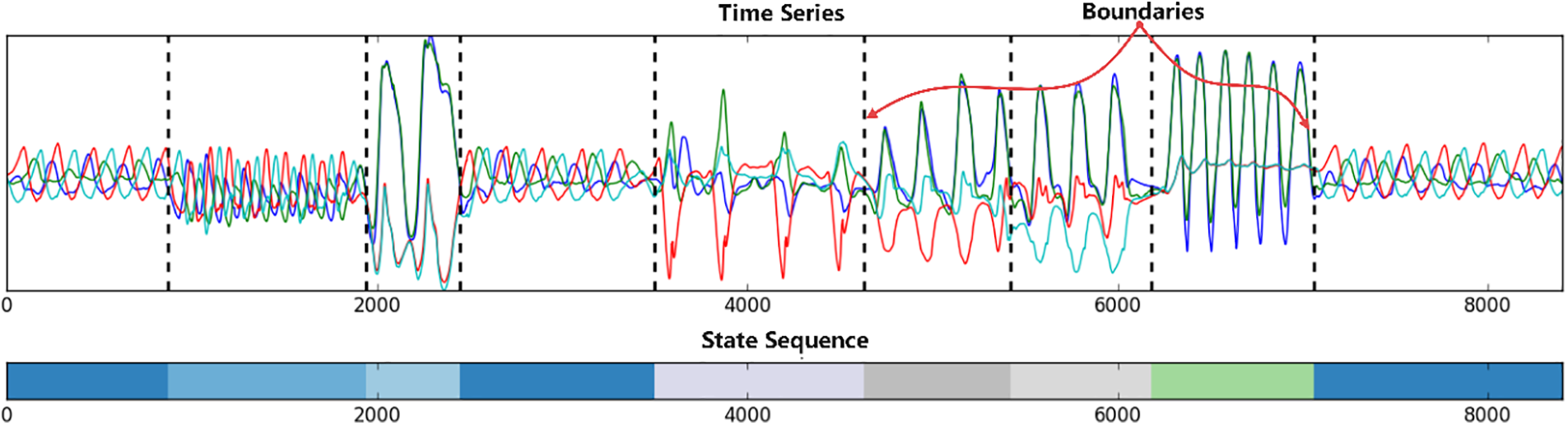
Figure 1: An example of boundary detection and state detection

The motivations and contributions of this paper are three-fold:

•   Existing surveys mainly focus on change point detection (CPD) methods while overlooking recent advances in boundary detection (BD) and state detection (SD) methods. Particularly, these surveys failed to capture the recent advances in BD and SD methods. This paper aims to fill this gap by reviewing recent advances in BD and SD methods;

•   The term “segmentation” is overloaded in the context of time series analysis and can refer to CPD, BD, and SD methods, but lacks a unified framework for describing these methods. This paper aims to clarify their differences and relationships, as well as provide a unified description under the framework of time series segmentation;

•   The inherent principles and evaluation manner of SD and BD differ greatly, we categorize BD and SD methods based on their underlying techniques/models, discuss the differences in evaluating BD and SD methods, and appeal to more comprehensive evaluation for BD and SD methods.

The rest of this paper is organized as follows. In Section 2, we introduce basic concepts and formulate the time series segmentation problem; In Section 3, we introduce popular datasets and commonly used metrics for evaluating BD and SD methods. In Section 4, we classify existing BD and SD methods according to their underlying techniques/models and introduce them separately, with a particular focus on the milestones that have shaped the development trajectory of a category of methods. We conclude the recent advances in time series segmentation in Section 5.

2  Problem Formulation

There are multiple forms of definitions for time series in the context of time series analysis. In the topic of time series segmentation, we usually consider multivariate time series, which is generally treated as a sequence of multivariate observations. In this paper, we use the definitions presented in [2].

DEFINITION 1. (Time Series) Multivariate time series is a sequence of multivariate observations: x={xi}i=1N, where xi∈Rd is the i-th multivariate observation, N is the length of the time series, d is the number of channels/dimensions.

With the above definition, a subsequence starts from time a and ends at time b can be denoted as xa:b, if necessary, a superscript j can be used to index the channel.

The concept of state is abstract and encompassing, relating to contextual interests and cannot be strictly defined by explicit rules. Otherwise, states could arguably be identified using handcrafted features. An abstract definition provided by [2] characterizes state by its temporal behavior.

DEFINITION 2. (State) A state is a subsequence with potential semantic value in real-world, which generally shows high internal similarity, such as repetitive patterns and similar statistical characteristics.

The concept of state sequence is established by indexing the states of a multivariate time series in [2].

DEFINITION 3. (State Sequence) A state sequence is essentially an index sequence that indicates which state a time point xi belongs to, which can be denoted as s={si|i∈N+,i≤N,si∈S}, where S is the set of indices {0, 1, …}.

With the above definitions, we can now formally formulate the boundary detection and state detection problem. Given a multivariate time series x, the goal of boundary detection is to find a set of boundary points ℬ={bi}, where the subsequences on either side of each boundary point belong to different states; The aim of state detection is to infer the corresponding sequence of states s, with the boundaries as a naturally formed byproduct.

3  Evaluation Metrics and Datasets

Before reviewing time series segmentation methods, it is essential to introduce the criteria for assessing these methods and the datasets used. Understanding the details of the evaluation criteria and datasets helps practitioners to test the methods at hand before real-world deployment. In generally, the datasets used for evaluating BD and SD methods are universal, but there are differences in the evaluation metrics. This section provides an introduction to the primary metrics and commonly used datasets for evaluating BD and SD methods. The evaluation metrics include F-measure, error, and several clustering metrics, each measuring different aspects of the performance. Regarding datasets, we will discuss several widely used public datasets that cover various application domains such as EEG and activity data. The selection of these metrics and datasets is crucial for a fair and comprehensive evaluation of different methods.

3.1 Evaluation Metrics

The evaluation of time series segmentation mainly revolves around two core aspects. Firstly, it entails evaluating the performance in identifying boundary points, and secondly, the performance in assigning states to time points. Subsequently, we will introduce the evaluation metrics for each of these aspects separately.

3.1.1 Metrics for Boundary Detection

Many works use the F-Measure (i.e., F1-score/Precision/Recall) to evaluate the performance of boundary point detection:

F1=2×Precision×RecallPrecision+Recall,Precision=#TP#TP+#FP,Recall=#TP#TP+#FN(1)

where #TP is the number of true positive, #FP is the number of false positive, #FN is the number of false negative.

However, as pointed out by Lin et al. [20], this manner lacks tolerance for trivial differences between ground truth and prediction. For example, the ground truth boundary for two segments is located at 10000, but an algorithm predicts a boundary at location 10001. In practice, this can definitely be considered as a successful prediction, because even in the ground truth, there are usually small errors, and state transitions are not instantaneous, predictions near the ground truth boundary points should also be considered as correct. However, this case will be counted as a false positive (FP) in the above manner.

A simple way to mitigate the above question is to add a window to bracket the ground truth. When a predicted boundary falls into a specified time window of the ground truth boundaries, it is counted as a TP; When a predicted boundary falls outside the time window of any ground truth boundaries, it is counted as a FN; When multiple predicted boundaries fall within the time window of a ground truth boundary, only the closest prediction will be counted as a TP, the others will be counted as FP. However, Gharghabi et al. [5] argue that this only slightly mitigates the above issue, and will still penalize an algorithm whose prediction slightly beyond the scope of the window. Hence, reference [5] proposes a scoring function to measure the error between ground truth and predicted boundary points. The scoring function is formulated as the following formula in [9]:

error=1n⋅|cptspred|⋅∑p∈cptspredminp′∈cptsT|p−p′|(2)

where cptspred is the predicted boundary points, cptsT is the ground truth boundary points, with each location in [1…n]. The error ranges in [0,1].

Although the above methods can further alleviate the problems in evaluation, there are still shortcomings. As pointed out in [9]: this measure does not perform a bipartite matching, as multiple predicted boundaries may be matched to the same ground truth boundaries. This can be seen as a disadvantage. For easy understanding, let us give an extreme example, if a segmentation algorithm outputs multiple boundaries that are concentrated near a ground truth boundary, or only outputs one boundary and omits other boundaries, then its error will still be low, which is definitely a disadvantage.

Based on the above introduction and analysis, we believe that a more reasonable approach would be to simultaneously use F-Measure and the scoring function proposed in [5] for comprehensively evaluation, as in [4].

3.1.2 Metrics for State Detection

For state detection evaluation, the metrics are more intuitive, two commonly adopted metrics are the Adjusted Rand Index (ARI) and Normalized Mutual Information (NMI), which are two clustering evaluation metrics that intuitively measure the point-wise matching degree between prediction and ground truth [2,3]. Given the ground truth X and prediction Y, ARI and NMI can be calculated by:

NMI(X,Y)=2×I(X;Y)H(X)+H(Y)(3)

ARI(X,Y)=RI−E[RI]max(RI)−E[RI](4)

where I(⋅) is the mutual information, H(⋅) is the entropy, RI is the rand index, E denotes the expectation.

We notice that SD methods rarely use the metrics for evaluating BD methods as evaluation metrics, but focus more on the point-wise state assignment performance by using clustering metrics. We believe that incorporating BD metrics will make the evaluation of SD methods more comprehensive.

3.2 Datasets

UCR-SEG [5,21]: UCR-SEG is a collection of benchmark datasets, each corresponds to a univariate time series taken from the medical, insects, robots, etc. This benchmark is somewhat special as it was initially collected for evaluating boundary detection methods, usually only one time series of data is prepared for each domain, and the states in each time series is usually not repeated. This dataset is widely used to evaluate boundary detection methods.

TSSB [9]: This dataset is a superset of UCR-SEG, created by Schäfer et al. [9]. This dataset contains not only the original 32 time series from the UCR-SEG, but also 66 semi-synthetic time series created from UCR archive (a benchmark for time series classification). Specifically, the authors pick time series with obvious periodicity from the UCR archive and concatenate time series with the same class label to create segments with repeating temporal patterns and characteristics. Then the segments are concatenated to form time series with different states, the concatenate positions are marked as boundary points. For more details, please refer to [9].

WESAD [22]: This dataset is collected for detecting the stress and emotion states, e.g., neutral, stress, and amusement. WESAD is collected from multi-modal wearable sensors, which is composed of physiological and motion data from chest and wrist-worn sensors of 15 subjects. The sensor modalities include blood volume pulse, electrocardiogram, etc.

EyeState [23]: EyeState dataset is used for investigating how the eye state (open/closed) can be predicted by measuring brain waves with an EEG, which collects a corpus containing the activation strength of the 14 electrodes of a commercial EEG headset.

MoCap [24]: The MoCap dataset, published by the Carnegie Mellon Graphics Lab, contains various motion data on up to 144 subjects. These data were collected by multiple infrared cameras from humans wearing special clothing that has markers taped on. The raw data contains 62 channels corresponding to different parts of human body, and each data has a corresponding video to provide ground truth. MoCap is widely used in a large number of time series segmentation studies, e.g., [2].

ActRecTut [25]: ActRecTut contains acceleration data collected from sports activities. The data contains 24 channels, recording eight gestures of daily living.

PAMAP2 [26]: PAMAP2 is a physical activity monitoring dataset containing 18 different low-level and high-level physical activities (such as walking, cycling, playing soccer, etc.), performed by 9 subjects wearing 3 inertial measurement units (IMU) and a heart rate monitor. The dataset has been used for evaluating time series segmentation methods in references [2,4]. Each data record in PAMAP2 consists of 52 attributes corresponding to acceleration, temperature, etc.

USC-HAD [27]: USC-HAD aims at constructing a publicly available benchmark to compare the performance of activity recognition methods, which records well-defined low-level daily activities such as walk, run, lie on bed, stand and drink water. USC-HAD has been widely used for comparing the performance of time series segmentation methods [2,4]. USC-HAD records 5 independent trials of 14 subjects and 12 daily activities with the sensing hardware attached to the subjects. The data records in USC-HAD contain 6 channels corresponding to the 3-axis accelerometer and gyroscope. There are also many activity recognition datasets alike to UCR-SEG that can be used for evaluating time series segmentation methods [28–31].

Synthetic: There are also some synthetic datasets used for evaluating segmentation performance, which are generally published together with segmentation methods. Wang et al. [2] use a tool called TSAGen [32] to generate a synthetic time series dataset, wherein the shape characteristics of segments reflect the states, each lasting for a random period.

Understanding the details of the evaluation criteria and datasets helps in better comprehending the performance and applicability of different methods, especially helpful for practitioners to test their methods before real-world deployment. Having introduced the evaluation metrics and datasets, we now move on to discuss the recent advances in BD and SD methods. By analyzing these methods in detail, we aim to highlight their strengths, weaknesses, and suitable application scenarios, thus aiding researchers and practitioners in selecting the appropriate methods for their specific problems.

4  Recent Advances

In this section, we introduce existing methods and categorize them based on their foundational models, boundary detection and state detection methods are introduced separately. Within each method type, our focus will be on highlighting key milestones and introducing notable techniques that have shaped the evolutionary path of these methodologies. Simultaneously, we will analysis the advantages and disadvantages inherent in each of these methods. We will also summarize the key attributes of these methods in segmentation scenarios that are of concern to users, such as whether a method requires the specification of the number of states/segments, and whether a method is for univariate or multivariate time series.

Categories of Methods: As aforementioned, we divide the time series segmentation methods into BD methods and SD methods. Then we subdivide the BD methods into profile-based methods and entropy-based methods; The state detection methods are further divided into traditional methods (which contains Markov models and clustering-based methods), compression-based methods, and hybrid methods. The categorization of these methods is summarized in Table 1.

4.1 State Detection Methods

4.1.1 Statistical Methods

The traditional statistical time series segmentation methods are mainly based on Markov models, e.g., Hidden Semi-Markov Model (HSMM) [35] and Markov Random Fields (MRF) [39] and their variants [36]. In this part, we start with the classic Hidden Markov Model (HMM) [40], introducing its application in the context of time series segmentation. Subsequently, we provide a review on some key variants to introduce how they are augmented to better accommodate the segmentation task.

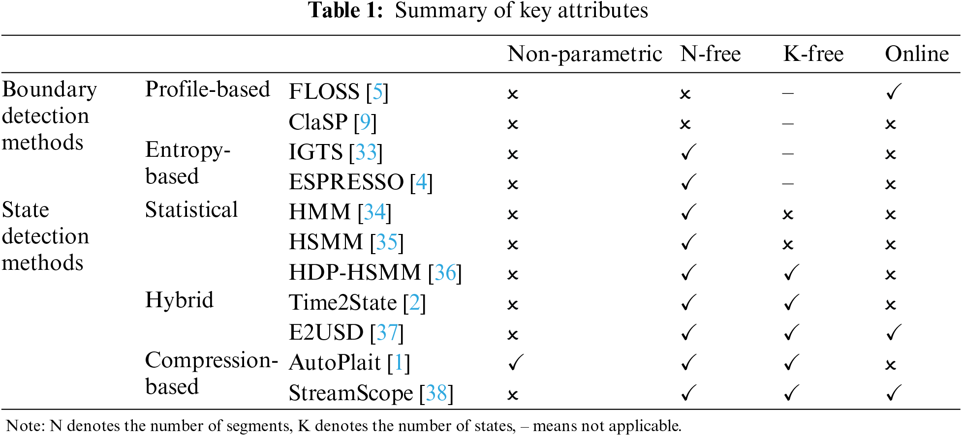
Hidden Markov Models. Hidden Markov Model (HMM) [34,40] is a well-known latent state inference model used to describe a Markov process with hidden unknown parameters, which works by inferring the hidden parameters of the process from observable variants. HMM can be applied to time series segmentation tasks by assuming the corresponding state sequences of observations as hidden variables. The HMM model is illustrated in Fig. 2.

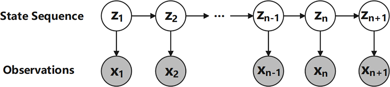
Figure 2: Hidden Markov model

A Hidden Markov Model (HMM) can be formulated as a 5-tuple Ω=(S, O, A, B,π), where S={Si, S2, …, SK} is the hidden state set, O={O1, O2, …, OM} is the observation set, A=(ai,j) is the transition probability matrix with ai,j indicating the probability of transition from Si to Sj, B=(bj,k) is the emission probability matrix with bj,k indicating the probability of observing symbol Ok while in state Sj, π=[πi] is the initial state distribution with πi indicating the probability of starting in state Si. The HMM is fully defined by its states, observations, transition probabilities, emission probabilities, and initial state distribution.

There are three core problems of HMM, which are the evaluation, decoding, and learning problem, respectively:

1) Evaluation problem: Given an HMM and an observation sequence, the evaluation problem is to determine the probability of observing this observation sequence.

2) Decoding problem: Given an HMM, the decoding problem is to find the most likely sequence of hidden states for observing this observation sequence. For the decoding problem, the commonly used method is the Viterbi algorithm [41], which is a dynamic programming algorithm used to find the most probable sequence of hidden states given an observation sequence and the model parameters.

3) Learning problem: Given an observation sequence, the learning problem is to estimating the parameters of an HMM. For the learning problem, the common approach is to use the Expectation-Maximization (EM) algorithm [42] to estimate the parameters of the HMM. In each iteration, the EM algorithm alternates between the E-step (Expectation Step) and the M-step (Maximization Step), updating the model parameters to maximize the log-likelihood of the observation sequence.

In the context of time series segmentation, we mainly focus on the decoding and learning problem. Given an observation sequence, the first step is to fit a HMM on the observation sequence, the corresponding hidden state sequence is the desired state sequence for segmenting the time series. On homogeneous datasets, fitting the model once typically suffices, enabling its use for decoding other data. Yet, with heterogeneous datasets, the performance may decline, often necessitating the fitting of a distinct HMM model for each time series.

Hidden Semi-Markov Models. As a basic model for time series segmentation, HMMs assume that each state emits an observation at each time step and transitions to a new state in the next time step. However, in many real-world scenarios, the duration spent in each state can vary significantly, and transitions between states may not occur at every time step. HMMs fail to capture such temporal dependencies with fixed-duration states. To overcome this deficiency, many variants of HMM are proposed, e.g., variable-duration HMMs, explicit-duration HMMs, segment HMMs, and multigram.

Among these variants, a noteworthy model is the Hidden Semi-Markov Model (HSMM) [35,43], which is a strict generalizations of variable-duration HMMs. HSMM is an extension of HMM that considers the explicit probability distribution of state duration, as described in [35], an HSMM is like an HMM except each state can emit a sequence of observations. The HSMM model is illustrated in Fig. 3, and the unified and detailed surveys of HSMMs can be found in [43].

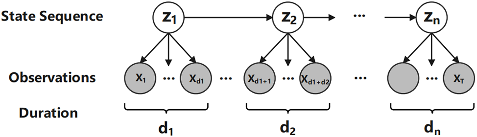
Figure 3: Hidden semi-Markov model

In summary, the motivation behind HSMM stems from the limitations of the traditional HMMs in accurately capturing temporal dynamics with variable durations. HSMMs aim to address this limitation by allowing states to have variable durations. By introducing explicit modeling of state durations, HSMMs provide a more flexible framework for capturing complex temporal patterns in sequential data.

Nonparametric Bayesian Hidden Semi-Markov Models. HSMMs extend HMMs by modeling the duration of states, but still requires the specification of the number of states (K). Recent advances in non-parametric Bayesian methods have been used to estimate the number of states automatically, such as the HDP-HMM [44,45] and HDP-HSMM [36]. References [36,46] compared to HDP-HMM, HDP-HSMM is more suitable for handling real-world data than the HDP-HMM due to its capability to effectively tackle the non-Markovian characteristics often present in such data. The HDP-HMM fails to account for these features, which can result in non-Markovian behavior causing an inflated number of states and unrealistically swift transition dynamics, particularly in nonparametric contexts.

The HDP-HSMM is a non-parametric Bayesian extension of HSMM, which uses the hierarchical Dirichlet process (HDP) [47,48] as the prior for the number of states. HDP is a nonparametric prior and a distribution over a set of random probability measures, which allows the mixture models to share components [47]. It should be noted that even with the implementation of HDP, both HDP-HMM and HDP-HSMM are not genuinely automatic methods in the strictest sense, as they typically necessitate the specification of a concentration parameter α for the hierarchical Dirichlet process. However, α generally exhibits considerable adaptability and does not require excessive fine-tuning to adapt to the data.

TICC. Toeplitz Inverse Covariance-based Clustering (TICC) stands as a clustering method, which is based on Markov model and Toeplitz inverse covariance. Unlike traditional clustering methods [49–53], the cluster in TICC is defined by a correlation network, i.e., MRF, that characterizing the interdependencies between observations, which enables better modeling of the context of time series. Based on the graphical representation, TICC simultaneously segments and clusters the time series data by alternating minimization, using a variation of the expectation maximization (EM) algorithm.

4.1.2 Representation Learning-Based Methods

Representation learning-based methods [2,37,54] are usually hybrid methods that incorporate multiple techniques. They use representation learning techniques to represent the raw data and conduct segmentation on the representations through clustering techniques. Representation learning [55–59] uses encoders (usually neural networks [60,61]) to learn distinguishable representations from raw data and maps them into a low-dimensional embedding space, thus benefits downstream tasks.

Time2State utilizes the advancements in time series representation learning for effective and efficient time series state detection. The architecture of Time2State is shown in Fig. 4, Time2State uses self-supervised leaning methods to learn an encoder. The encoder is trained by a newly proposed loss function, namely, LSE-Loss. During the training process, Time2State randomly samples multiple sets of consecutive windows from the time series, with each window and its consecutive windows as positive samples and other randomly sampled windows as negative samples. Subsequently, it calculates the embedding center of consecutive windows, and jointly maximizing the distance between embedding centers and minimizing the distance between the embeddings of consecutive windows through the LSE-Loss. Once the encoder is learned, it utilizes a sliding window to slide over the entire time series at a step size s, at the same time, all time windows are encoded in to a low-dimensional embedding space. Then a clustering component is applied on the embeddings to assign clustering labels. The clustering method used in Time2State is the Dirichlet Process Gaussian Mixture Model (DPGMM), which does not require the specification of K, but a concentration parameter α that determines the discreteness degree of the random measure G used in DPGMM. Since a time point may be covered by multiple window, the clustering labels are assigned to each time point by majority voting.

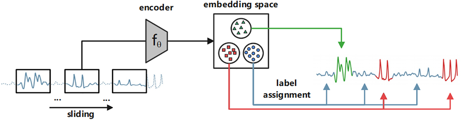
Figure 4: The architecture of Time2State

However, as pointed out by Lai et al. [37], there are two main problems in existing works. First, randomly sampling causes insufficient attention to false negatives, thus hampers model convergence and accuracy. Second, existing methods only emphasize offline non-streaming deployment. For the first problem, E2USD has further improved performance by introducing advanced representation learning strategies on the Time2State architecture. Specifically, it proposes a similarity-based negative sampling strategy, which selects genuinely dissimilar negative pairs via evaluating seasonal and trend similarities for each pair and retaining the least similar ones as negative samples. For the second problem, although adapting Time2State to online scenarios is not difficult, as it only requires encoding the new context (a time window) and re-clustering the embeddings at the arrival of each or several time points, but this undoubtedly increases computational overhead. E2USD proposes a new mechanism to adapt this architecture to online scenarios by adding an adaptive threshold and postpone clustering. Specifically, E2USD maintains an adaptive threshold τ, whenever a new sample arrives, the embedding is calculated for its context. Clustering operations are only performed when the similarity between the embedding of arrival sample and the previous sample is lower than the threshold. Otherwise, the state remains unchanged. This operation can greatly reduce redundant clustering and computational costs.

4.1.3 Compression-Based Methods

Compression-based hybrid methods are also a noteworthy category, which utilize the minimum description length (MDL) [62,63] to segment time series. MDL can be simply expressed as follows: among the given hypotheses, the hypothesis that can produce the best compression effect is optimal. Given a set of models ℳ, the best model M∈ℳ is the one that minimizes L(M)+L(D|M), where L(M) is the length (in bits) of the description of M, L(D|M) is the length of the data encoded with model M. It is worthy noting that, as pointed out in [1], compression is not the goal, but a means. These methods search for segments that can compactly describe data by focusing on the MDL.

Tatti et al. utilize MDL to segment discrete event sequence by using code table as the model, but cannot handle multivariate time series with continuous value [63]. AutoPlait [1] uses Multi-Level Chain Model (MLCM) as the model and design novel cost function to describe the data, wherein each regime is modeled by HMM. With the above new mechanism, AutoPlait has achieved promising results in segmenting multivariate time series, however, it is an offline method. StreamScope [38,64] is another work by the authors of AutoPlait, which also employs HMM and MDL to summarize and compress data. The difference between StreamScope and AutoPlait is that StreamScope can work in an online manner. To achieve the goal of working online, a new cost function has been proposed in StreamScope to incrementally calculate the increased cost when new samples arrive.

4.2 Boundary Detection Methods

In the recent advancements of BD methods, two categories of methods are noteworthy, which are the profile-based methods and entropy-based methods, respectively.

Profile-Based Methods. Profile (e.g., Matrix Profile, Neighbor Profile, and Classification Score Profile [9,65–68]) is a kind of data infrastructure for pattern/motif mining in time series data. It has proven effective for time series segmentation [5,9]. In [5], a type of curve called Corrected Arc Cross (CAC) was first extracted from the matrix profile. Subsequently, Schäfer et al. [9] proposed a concept called the classification score curve (CSP). In this paper, we collectively refer to these curves as “profile curves”. The profile curve is a concept that encompassing local and global similarity in a long-range time series, which usually exhibits high or low values near the segmentation point.

Profile-based methods utilize the profile curve to split time series into non-overlapping segments, which usually can only detect the boundaries of segments. As a general pipeline, profile-based methods first extract the profile curve from raw data; then, they search for boundaries by finding the local maxima or minima on the extracted profile curve. An example of a profile curve is shown in Fig. 5.

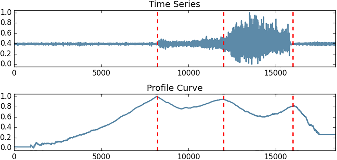
Figure 5: An example of profile-based method

Gharghabi et al. [5] first proposed the CAC curve, which uses the matrix profile as the infrastructure to calculate the nearest neighbor position for each fixed-size subsequence, with each subsequence having an arc pointing to its nearest neighbor in the data structure. After counting how many edges each subsequence is pointed to and a correction operation, the CAC curve is obtained. FLOSS is based on the core observation/assumption that subsequences in the boundary-point region are usually pointed to by very few arcs because most subsequences can find their nearest neighbors within their own segment, so a lower CAC value can be expected near the segment boundaries. FLOSS then finds the boundaries by searching for the local minima in the CAC curve. The design of FLOSS is based on univariate time series, but the authors propose a method to extend it to multivariate time series by averaging the profile curves corresponding to each channel in the multivariate time series and find boundaries on this overall profile curve. The case studies in [5] show the effectiveness of this strategy. It should also be noted that in the native algorithm and code implementation of FLOSS, it is necessary to specify the number of segments (N) as a parameter.

Schäfer et al. [9] proposed the classification score profile (ClaSP), which first partitions a time series into overlapping windows, then generates hypothetical split for increasing offsets. Subsequently, each split is transformed into a binary classification problem, where classifiers are trained based on the features extracted from each window. Finally, ClaSP uses cross-validation score as the measure to assess the difference between the left and right splits, thereby deriving ClaSP.

A major improvement of ClaSP over profile-based methods is that it proposes a recursive strategy to find boundary points upon the profile curve. In FLOSS, a simple method is used to extract local maxima/minima locations from the profile curve. This method only needs to run FLOSS once, but requires setting an exclusion zone to prevent matching values near the peak. In ClaSP, a recursive strategy is adopted where it selects only the global maximum each time. The time series is then divided into two parts based on this value, and ClaSP is recursively run on the newly obtained parts, until the desired number of boundaries are generated.

Entropy-Based Methods. IGTS [33] is an information gain-based method based on the concept of entropy. The authors propose an information gain-based cost function and two optimization strategies to find the best set of boundary points, at the same time, a heuristic method to find the best number of segments (N) is provided. The loss function considered in is as follows:

ℒ=H(S)−∑i=0ksiSH(si)(5)

where si∈S is the segments, H(⋅) is the entropy.

To optimize the above loss function, the authors propose a TopDown approach and a dynamic programming approach. According to [33], dynamic programming approach is able to detect global optima but is slower; On the other hand, TopDown optimization a trade-off between time and accuracy that is faster while cannot guarantee to provide the global optima. The TopDown approach is a greedy method, which runs in a hierarchical and greedy manner by treating the time series as a single segment and choose the split that reduces the total cost most as the in each step. The estimation of the number of segments N in IGTS is alike to the estimation of the number of clusters in clustering methods, i.e., find the ‘‘knee point’’ in evaluation metric. IGTS uses information gain as the evaluation metric and finds the point of maximum curvature (knee point) as N. For more details about IGTS, please refer to [33].

ESPRESSO [4] is a combination of shape-based and entropy-based methods. The search space for candidate boundaries in IGTS is large, resulting in high computational overhead. ESPRESSO proposes using profile-based (shape-based) methods mentioned above to propose candidate boundaries, thereby reducing the search space for boundaries, and then using entropy-based methods for optimization.

5  Conclusion

Time series segmentation plays a key role in time series analysis, which facilitates many downstream technologies, such as pattern recognition, event detection, etc. This paper categorizes time series segmentation methods into three types: change point detection, boundary detection, and state detection methods. Although many literature reviews have focused on time series segmentation technology, they mainly focus on change point detection methods, neglecting the advancements in boundary detection and state detection. This paper fills this gap by focusing on the advances in boundary detection and state detection methods, subdividing boundary detection methods and state detecting methods, and highlight review on the milestones that have shaped the development trajectory of a category of methods. In addition, we have also reviewed the evaluation metrics and datasets for boundary detection methods and state detection methods.

Acknowledgement: The authors would like to express their gratitude to the editors and reviewers for their detailed review and insightful advice.

Funding Statement: This work is supported by the National Key Research and Development Program of China (2022YFF1203001), National Natural Science Foundation of China (Nos. 62072465, 62102425), the Science and Technology Innovation Program of Hunan Province (Nos. 2022RC3061, 2023RC3027).

Author Contributions: Study conception and design: Chengyu Wang, Xionglve Li; draft manuscript preparation: Chengyu Wang, Xionglve Li; supervision: Tongqing Zhou, Zhiping Cai. All authors reviewed the results and approved the final version of the manuscript.

Availability of Data and Materials: This article does not involve data availability and this section is not applicable.

Conflicts of Interest: The authors declare that they have no conflicts of interest to report regarding the present study.

References

1. Y. Matsubara, Y. Sakurai, and C. Faloutsos, “AutoPlait: Automatic mining of co-evolving time sequences,” presented at the ACM SIGMOD Int. Conf. Manag. Data, New York, NY, USA, 2014. doi: 10.1145/2588555.2588556. [Google Scholar] [CrossRef]

2. C. Wang, K. Wu, T. Zhou, and Z. Cai, “Time2State: An unsupervised framework for inferring the latent states in time series data,” Proc. ACM Manag. Data., vol. 1, no. 1, pp. 17:1–17:18, 2023. doi: 10.1145/3588697. [Google Scholar] [CrossRef]

3. D. Hallac, S. Vare, S. Boyd, and J. Leskovec, “Toeplitz inverse covariance-based clustering of multivariate time series data,” presented at the 23rd ACM SIGKDD Int. Conf. Knowl. Discov. Data Mining, New York, NY, USA, 2017. doi: 10.1145/3097983.3098060. [Google Scholar] [CrossRef]

4. S. Deldari, D. Smith, A. Sadri, and F. Salim, “ESPRESSO: Entropy and shape aware time-series segmentation for processing heterogeneous sensor data,” Proc. ACM Interact. Mob. Wearable Ubiquitous Technol., vol. 4, no. 3, pp. 77:1–77:24, 2020. doi: 10.1145/3411832. [Google Scholar] [CrossRef]

5. S. Gharghabi et al., “Domain agnostic online semantic segmentation for multi-dimensional time series,” Data Min. Knowl. Discov., vol. 33, pp. 96–130, 2019. doi: 10.1007/s10618-018-0589-3. [Google Scholar] [PubMed] [CrossRef]

6. S. Aminikhanghahi and D. Cook, “A survey of methods for time series change point detection,” Knowl. Inf. Syst., vol. 51, no. 2, pp. 339–367, 2017. doi: 10.1007/s10115-016-0987-z. [Google Scholar] [PubMed] [CrossRef]

7. E. Ghaderpour, S. Pagiatakis, and Q. Hassan, “A survey on change detection and time series analysis with applications,” Appl. Sci., vol. 11, no. 13, 2021. doi: 10.3390/app11136141. [Google Scholar] [CrossRef]

8. C. Truong, L. Oudre, and N. Vayatis, “Selective review of offline change point detection methods,” Signal Process., vol. 167, pp. 107299, 2020. doi: 10.1016/j.sigpro.2019.107299. [Google Scholar] [CrossRef]

9. P. Schäfer, A. Ermshaus, and U. Leser, “ClaSP—time series segmentation,” presented at the 30th ACM Int. Conf. Inf. Knowl. Manag., New York, NY, USA, 2021, pp. 1578–1587. doi: 10.1145/3459637.3482240. [Google Scholar] [CrossRef]

10. J. Harguess and J. Aggarwal, “Semantic labeling of track events using time series segmentation and shape analysis,” presented at the 16th IEEE Int. Conf. Image Process. (ICIPCairo, Egypt, 2009, pp. 4317–4320. doi: 10.1109/ICIP.2009.5413671. [Google Scholar] [CrossRef]

11. P. Wang, H. Wang, and W. Wang, “Finding semantics in time series,” presented at the ACM SIGMOD Int. Conf. Manage. Data, Athens, Greece, 2011, pp. 385–396. doi: 10.1145/1989323.1989364. [Google Scholar] [CrossRef]

12. E. Ghaderpour, B. Antonielli, F. Bozzano, G. Mugnozza, and P. Mazzanti, “A fast and robust method for detecting trend turning points in InSAR displacement time series,” Comput. Geosci., vol. 185, pp. 105546, 2024. doi: 10.1016/j.cageo.2024.105546. [Google Scholar] [CrossRef]

13. D. Masiliūnas, N. Tsendbazar, M. Herold, and J. Verbesselt, “BFAST lite: A lightweight break detection method for time series analysis,” Remote Sens., vol. 13, no. 16, 2021. doi: 10.3390/rs13163308. [Google Scholar] [CrossRef]

14. E. Ghaderpour et al., “Least-squares wavelet analysis of rainfalls and landslide displacement time series derived by PS-InSAR,” presented at the Int. Conf. Time Ser. Forecast., Gran, Canaria, Spain, 2022, 117–132. doi: 10.1007/978-3-031-40209-8_9. [Google Scholar] [CrossRef]

15. E. Ghaderpour and S. Pagiatakis, “Least-squares wavelet analysis of unequally spaced and non-stationary time series and its applications,” Math. Geosci., vol. 49, pp. 819–844, 2017. doi: 10.1007/s11004-017-9691-0. [Google Scholar] [CrossRef]

16. C. Heil and D. Walnut, “Continuous and discrete wavelet transforms,” SIAM Rev., vol. 31, no. 4, pp. 628–666, 1989. doi: 10.1137/1031129. [Google Scholar] [CrossRef]

17. O. Rioul and P. Duhamel, “Fast algorithms for discrete and continuous wavelet transforms,” IEEE Trans. Inf. Theory, vol. 38, no. 2, pp. 569–586, 1992. doi: 10.1109/18.119724. [Google Scholar] [CrossRef]

18. G. Rilling, P. Flandrin and P. Goncalves, “On empirical mode decomposition and its algorithms,” presented at the IEEE-EURASIP Workshop on Nonlinear Signal and Image Process., Zagreb, Croatia, 2003, pp. 8–11. [Google Scholar]

19. A. Zeiler, R. Faltermeier, I. Keck, A. Tomé, C. Puntonet and E. Lang, “Empirical mode decomposition-an introduction,” presented at the Int. Joint Conf. Neural Netw. (IJCNNBarcelona, Spain, 2010, pp. 1–8. [Google Scholar]

20. J. Lin, M. Karg, and D. Kulić, “Movement primitive segmentation for human motion modeling: A framework for analysis,” IEEE Trans. Hum. Mach. Syst., vol. 46, no. 3, pp. 325–339, 2016. doi: 10.1109/THMS.2015.2493536. [Google Scholar] [CrossRef]

21. S. Gharghabi, Y. Ding, C. Yeh, K. Kamgar, L. Ulanova and E. Keogh, “Matrix profile VIII: Domain agnostic online semantic segmentation at superhuman performance levels,” presented at the 2017 IEEE Int. Conf. Data Mining (ICDMNew Orleans, LA, USA, 2017, pp. 117–126. doi: 10.1109/ICDM.2017.21. [Google Scholar] [CrossRef]

22. J. Heinisch, C. Anderson, and K. David, “Angry or climbing stairs? Towards physiological emotion recognition in the wild,” presented at the 2019 IEEE Int. Conf. Pervasive Comput. Commun. Workshops (PerCom WorkshopsKyoto, Japan, 2019, pp. 486–491. [Google Scholar]

23. O. Rösler and D. Suendermann, “A first step towards eye state prediction using eeg,” in Proc. of the AIHLS, Istanbul, Turkey, 2013, vol. 1, pp. 1–4. [Google Scholar]

24. MoCap. 2024. Accessed: Jul. 3, 2024. [Online]. Available: http://mocap.cs.cmu.edu [Google Scholar]

25. U. Von Luxburg, “A tutorial on spectral clustering,” Stat. Comput., vol. 17, no. 4, pp. 395–416, 2007. doi: 10.1007/s11222-007-9033-z. [Google Scholar] [CrossRef]

26. A. Reiss and D. Stricker, “Introducing a new benchmarked dataset for activity monitoring,” presented at the 16th Int. Symp. Wearable Comput., Newcastle, UK, 2012, pp. 108–109. doi: 10.1109/ISWC.2012.13. [Google Scholar] [CrossRef]

27. M. Zhang and A. Sawchuk, “USC-HAD: A daily activity dataset for ubiquitous activity recognition using wearable sensors,” presented at the ACM Conf. Ubiquitous Comput., New York, NY, USA, 2012, pp. 1036–1043. doi: 10.1145/2370216.2370438. [Google Scholar] [CrossRef]

28. D. Roggen et al., “Collecting complex activity datasets in highly rich networked sensor environments,” Presented at the 2010 Seventh Int. Conf. Netw. Sens. Syst. (INSSKassel, Germany, 2010, pp. 233–240. [Google Scholar]

29. A. Yang, R. Jafari, S. Sastry, and R. Bajcsy, “Distributed recognition of human actions using wearable motion sensor networks,” J. Ambient Intell. Smart Environ., vol. 1, no. 2, pp. 103–115, 2009. doi: 10.3233/AIS-2009-0016. [Google Scholar] [CrossRef]

30. E. Tapia, S. Intille, L. Lopez, and K. Larson, “The design of a portable kit of wireless sensors for naturalistic data collection,” presented at the Pervasive Comput. 4th Int. Conf., Dublin, Ireland, 2006, pp. 117–134. [Google Scholar]

31. F. De la Torre et al., “Guide to the carnegie mellon university multimodal activity CMU-MMAC database,” 2024. Accessed: Jul. 3, 2024. [Online]. Available: https://www.ri.cmu.edu/publications/guide-to-the-carnegie-mellon-university-multimodal-activity-cmu-mmac-database/ [Google Scholar]

32. C. Wang, K. Wu, T. Zhou, G. Yu, and Z. Cai, “TSAGen: Synthetic time series generation for KPI anomaly detection,” IEEE Trans. Netw. Serv. Manag., vol. 19, no. 1, 2022. doi: 10.1109/TNSM.2021.3098784. [Google Scholar] [CrossRef]

33. A. Sadri, Y. Ren, and F. Salim, “Information gain-based metric for recognizing transitions in human activities,” Pervasive Mob. Comput., vol. 38, pp. 92–109, 2017. doi: 10.1016/j.pmcj.2017.01.003. [Google Scholar] [CrossRef]

34. S. Eddy, “Hidden markov models,” Curr. Opin. Struct. Biol., vol. 6, no. 3, pp. 361–365, 1996. [Google Scholar] [PubMed]

35. K. Murphy, “Hidden semi-markov models (HSMMs),” 2002. Accessed: Jul. 3, 2024. [Online]. Available: https://citeseerx.ist.psu.edu/document?repid=rep1&type=pdf&doi=a2125e4fba6c69ff7a6d247bcf04312bb2b79606 [Google Scholar]

36. M. Johnson and A. Willsky, “Bayesian nonparametric hidden semi-markov models,” J. Mach. Learn. Res., vol. 14, no. 20, pp. 673–701, 2013. [Google Scholar]

37. Z. Lai, H. Li, D. Zhang, Y. Zhao, W. Qian and C. Jensen, “E2Usd: Efficient-yet-effective unsupervised state detection for multivariate time series,” presented at the ACM on Web Conf. 2024, New York, NY, USA, 2024, pp. 3010–3021. doi: 10.1145/3589334.3645593. [Google Scholar] [CrossRef]

38. K. Kawabata, Y. Matsubara, and Y. Sakurai, “StreamScope: Automatic pattern discovery over data streams,” presented at the First Int. Workshop on Exploiting Artif. Intell. Tech. for Data Manage., Houston, TX, USA, 2018, pp. 1–8. doi: 10.1145/3211954.3211959. [Google Scholar] [CrossRef]

39. P. Clifford, “Markov random fields in statistics,” in Disorder in Physical Systems: A Volume in Honour of John M. Hammersley, Berlin, Germany: Springer, 1990, pp. 19–32. [Google Scholar]

40. S. Eddy, “What is a hidden Markov model?” Nat. Biotechnol., vol. 22, no. 10, pp. 1315–1316, 2004. doi: 10.1038/nbt1004-1315. [Google Scholar] [PubMed] [CrossRef]

41. S. Benedetto and E. Biglieri, “Viterbi algorithm,” in Principles of Digital Transmission: With Wireless Applications, Oxford, UK: Oxford University Press, 2002, pp. 807–815. [Google Scholar]

42. C. Do and S. Batzoglou, “What is the expectation maximization algorithm?,” Nat. Biotechnol., vol. 26, no. 8, pp. 897–899, 2008. doi: 10.1038/nbt1406. [Google Scholar] [PubMed] [CrossRef]

43. S. Yu, “Hidden semi-Markov models,” Artif. Intell., vol. 174, no. 2, pp. 215–243, 2010. doi: 10.1016/j.artint.2009.11.011. [Google Scholar] [CrossRef]

44. M. Beal, Z. Ghahramani, and C. Rasmussen, “The infinite hidden Markov model,” Adv. Neural Inf. Process. Syst., vol. 14, pp. 1–8, 2001. [Google Scholar]

45. K. Murphy, “Dynamic bayesian networks,” 2002. Accessed: Jul. 3, 2024. [Online]. Available: https://webdocs.cs.ualberta.ca/~rgreiner/C-366/RG-2002-SLIDES/dbn-murphy.pdf [Google Scholar]

46. E. Fox, E. Sudderth, M. Jordan, and A. Willsky, “An HDP-HMM for systems with state persistence,” presented at the 25th Int. Conf. Mach. Learn., Helsinki, Finland, 2008, pp. 312–319. [Google Scholar]

47. Y. Teh, M. Jordan, M. Beal, and D. Blei, “Sharing clusters among related groups: Hierarchical dirichlet processes,” Adv. Neural Inf. Process. Syst., vol. 17, pp. 1–8, 2004. [Google Scholar]

48. Y. Teh, M. Jordan, M. Beal, and D. Blei, “Hierarchical dirichlet processes,” J. Am. Stat. Assoc., vol. 101, no. 476, pp. 1566–1581, 2006. doi: 10.1198/016214506000000302. [Google Scholar] [CrossRef]

49. M. Ankerst, M. Breunig, H. Kriegel, and J. Sander, “OPTICS: Ordering points to identify the clustering structure,” presented at the ACM SIGMOD Int. Conf. Manage. Data, New York, NY, USA, 1999, pp. 49–60. doi: 10.1145/304182.304187. [Google Scholar] [CrossRef]

50. M. Ester, H. Kriegel, J. Sander, and X. Xu, “A density-based algorithm for discovering clusters in large spatial databases with noise,” presented at the ACM SIGKDD Conf. Knowl. Discov. Data Mining, Portland, Oregon, 1996, pp. 226–231. [Google Scholar]

51. D. Steinley, “K-means clustering: A half-century synthesis,” Br. J. Math. Stat. Psychol., vol. 59, no. 1, pp. 1–34, 2006. doi: 10.1348/000711005X48266. [Google Scholar] [PubMed] [CrossRef]

52. J. Liu et al., “Optimal neighborhood multiple kernel clustering with adaptive local kernels,” IEEE Trans. Knowl. Data Eng., vol. 34, no. 6, pp. 2872–2885, 2022. doi: 10.1109/TKDE.2020.3014104. [Google Scholar] [CrossRef]

53. S. Wang et al., “Fast parameter-free multi-view subspace clustering with consensus anchor guidance,” IEEE Trans. Image Process., vol. 31, pp. 556–568, 2022. doi: 10.1109/TIP.2021.3131941. [Google Scholar] [PubMed] [CrossRef]

54. Nagano M, Nakamura T, Nagai T, Mochihashi D, Kobayashi I and W. Takano, “HVGH: Unsupervised segmentation for high-dimensional time series using deep neural compression and statistical generative model,” Front. Rob. AI, vol. 6, 2019. doi: 10.3389/frobt.2019.00115. [Google Scholar] [PubMed] [CrossRef]

55. E. Eldele et al., “Time-series representation learning via temporal and contextual contrasting,” presented at the Thirtieth Int. Joint Conf. Artif. Intell. (IJCAI2021, pp. 2352–2359. [Google Scholar]

56. J. Franceschi, A. Dieuleveut, and M. Jaggi, “Unsupervised scalable representation learning for multivariate time series,” presented at the Adv. Neural Inf. Process. Syst., Vancouver, BC, Canada, 2019, pp. 1–12. [Google Scholar]

57. A. Van den Oord, Y. Li, and O. Vinyals, “Representation learning with contrastive predictive coding,” arXiv preprint arXiv:1807.03748, 2018. [Google Scholar]

58. S. Tonekaboni, D. Eytan, and A. Goldenberg, “Unsupervised representation learning for time series with temporal neighborhood coding,” arXiv preprint arXiv:2106.00750, 2021. [Google Scholar]

59. Z. Yue et al., “Ts2Vec: Towards universal representation of time series,” presented at the AAAI Conf. Artif. Intell., 2022, pp. 8980–8987. [Google Scholar]

60. T. Zhou, Z. Cai, F. Liu, and J. Su, “In pursuit of beauty: Aesthetic-aware and context-adaptive photo selection in crowdsensing,” IEEE Trans. Knowl. Data Eng., vol. 35, no. 9, pp. 9364–9377, 2023. doi: 10.1109/TKDE.2023.3237969. [Google Scholar] [CrossRef]

61. Y. Shi, J. Xi, D. Hu, Z. Cai, and K. Xu, “RayMVSNet++: Learning ray-based 1D implicit fields for accurate multi-view stereo,” IEEE Trans. Pattern Anal. Mach. Intell., vol. 45, no. 11, pp. 13666–13682, 2023. doi: 10.1109/TPAMI.2023.3296163. [Google Scholar] [PubMed] [CrossRef]

62. A. Barron, J. Rissanen, and B. Yu, “The minimum description length principle in coding and modeling,” IEEE Trans. Inf. Theory, vol. 44, no. 6, pp. 2743–2760, 1998. doi: 10.1109/18.720554. [Google Scholar] [CrossRef]

63. N. Tatti and J. Vreeken, “The long and the short of it: Summarising event sequences with serial episodes,” presented at the 18th ACM SIGKDD Int. Conf. Knowl. Discov. Data Mining, Beijing, China, 2012, pp. 462–470. doi: 10.1145/2339530.2339606. [Google Scholar] [CrossRef]

64. K. Kawabata, Y. Matsubara, and Y. Sakurai, “Automatic sequential pattern mining in data streams,” presented at the 28th ACM Int. Conf. Inf. Knowl. Manage., Beijing, China, 2019, pp. 1733–1742. doi: 10.1145/3357384.3358002. [Google Scholar] [CrossRef]

65. Y. He, X. Chu, and Y. Wang, “Neighbor profile: Bagging nearest neighbors for unsupervised time series mining,” presented at the IEEE 36th Int. Conf. Data Eng. (ICDEDallas, TX, USA, 2020, pp. 373–384. doi: 10.1109/ICDE48307.2020.00039. [Google Scholar] [CrossRef]

66. F. Madrid, S. Imani, R. Mercer, Z. Zimmerman, N. Shakibay and E. Keogh, “Matrix profile XX: Finding and visualizing time series motifs of all lengths using the matrix profile,” presented at the IEEE Int. Conf. Big Knowl. (ICBKBeijing, China, 2019, pp. 175–182. doi: 10.1109/ICBK.2019.00031. [Google Scholar] [CrossRef]

67. C. Yeh, N. Kavantzas, and E. Keogh, “Matrix profile VI: Meaningful multidimensional motif discovery,” presented at the IEEE Int. Conf. Data Mining (ICDMBeijing, China, 2017, pp. 565–574. doi: 10.1109/ICDM.2017.66. [Google Scholar] [CrossRef]

68. C. Yeh et al., “Matrix profile I: All pairs similarity joins for time series: a unifying view that includes motifs, discords and shapelets,” presented at the IEEE 16th Int. Conf. Data Mining (ICDMBarcelona, Spain, 2016, pp. 1317–1322. doi: 10.1109/ICDM.2016.0179. [Google Scholar] [CrossRef]