Multivariate Time Series Anomaly Detection Based on Spatial-Temporal Network and Transformer in Industrial Internet of Things

Nomenclature

1  Introduction

The Industrial Internet of Things (IIoT) holds significant importance for the development of society. By providing network access, IIoT enhances the interconnectivity of industrial systems. However, this also makes IIoT more vulnerable to external attacks. The IIoT collects data through a variety of deployed sensors, monitoring the operational status of infrastructure, and by analyzing the data provided by these sensors, they provide real-time decision support for industrial control systems in fields such as aerospace, oil and gas, and water treatment [1,2]. Therefore, timely detection of sensor anomalies is crucial for ensuring the secure and stable operation of IIoT. Since the data generated by sensors are time series data, our main research task is focused on time series anomaly detection. This task aims to enhance the security and reliability of IIoT by identifying abnormal patterns in sensor data through advanced algorithms and models.

A variety of deep learning-based methods for identifying anomalies in time series have been developed. Many researchers utilized autoencoders for time series anomaly detection [3–5]. Generative Adversarial Networks (GANs) utilize trained generators and discriminators to detect anomalies [6,7]. Some models employ several networks working together for anomaly detection. OmniAnomaly [8] proposes stochastic recurrent neural networks to capture the normal time series distribution and identify anomalies using reconstruction probabilities. Park et al. [9] introduced a technique for detecting anomalies, utilizing a variational autoencoder and (long short-term memory) LSTM.

Due to the superior performance of the Transformer, it is studied in time series anomaly detection. Zhang et al. [10] proposed MBTGMM, and the framework acquires short and long temporal dependencies by the multi-branch Transformer. Then, density estimation and anomaly detection are performed by the Gaussian mixture model. Tuli et al. [11] proposed TranAD, the architecture based on the Transformer, and the feature is extracted by self-conditioning based on the focus score. The key element of the Transformer is self-attention, enabling the model to attend to various input positions, thereby effectively capturing the dependencies within the input and achieving good results in various tasks. Therefore, the Transformer is introduced into the proposed method. Nie et al. [12] and Yang et al. [13] proposed the channel-independent patch to enhance the local semantic information, allowing the Transformer to more effectively grasp both local and global information in the time series. Therefore, patching is introduced in our proposed model.

Although deep learning-based methods have achieved good results in anomaly detection, they have difficulties in capturing the relationships between different dimensions in time series. Therefore, the methods based on graph neural networks (GNNs) have been proposed [14–16]. Deng et al. [14] proposed GDN, where embeddings are used to construct the graph structure, and anomalies are identified based on the prediction obtained from the Graph Attention Networks (GATs). Chen et al. [15] proposed VGCRN, and the framework utilizes probabilistic generative networks and graph convolutional networks (GCNs) to capture dependencies within time series. Tang et al. [16] introduced the utilization of a Gated Recurrent Unit (GRU) within the framework of GATs for time series anomaly detection. Although the methods based on GNNs for anomaly detection can capture relationships between different dimensions, they have two issues. Firstly, when modeling time series, it is essential to consider the spatial correlations without neglecting the temporal correlations between sensors at the same time. Secondly, the model training and graph structure learning of these methods are conducted simultaneously, so the obtained model parameters and graph structure may not be optimal.

To cope with the above challenges, this paper proposes a time series anomaly detection method based on spatial-temporal network and Transformer. The method consists of four parts: the spatial-temporal network module, the Transformer module, the anomaly scoring module, and the adaptive graph structure learning module. The spatial-temporal network utilizes a temporal convolution network (TCN, based on dilated causal convolution) and a graph convolutional network to capture the temporal and spatial correlations of the time series. The Transformer module encodes the inputs using the encoder, thereby capturing the interdependencies between all positions in the input sequence. This allows for a better understanding of the semantics and structural information of the input sequence. Then, the decoder uses the internal representation of the time series generated by the encoder to produce the output sequence. The anomaly scoring module obtains the predicted values based on the output of the Transformer and determines anomalies based on the anomaly scores derived from the comparison between the predicted and observed values. The graph structure learning module comprises two components: model training and graph structure learning. The method alternately trains the model parameters and the graph structure learning to obtain the optimal model parameters and graph structure. The main contributions of this paper are summarized as follows:

•   We propose a novel time series anomaly detection method, based on spatial-temporal network and Transformer.

•   The spatial-temporal network utilizes a GCN to capture spatial relationships, while a TCN is employed to extract temporal relationships. Additionally, an improved Transformer model is used to achieve a deeper understanding and transformation of the time series data.

•   An adaptive graph structure learning method is introduced to obtain the optimal model parameters and graph structure.

•   A large number of experiments show that our approach achieves better performance than baselines.

The remainder of the paper is structured as follows: Section 2 summarizes the literature on time series anomaly detection. Section 3 elaborates on the proposed framework and describes its constituent parts. Section 4 details the experimental outcomes of the model. We conclude the paper and suggest directions for future work in Section 5.

2  Related Work

Many time series anomaly detection methods have been proposed. These methods can be divided into traditional methods and deep learning-based methods. Traditional methods can be identified as distance-based [17], linear-based [18], density-based [19], wavelet-based [20,21], classification-based [22], and Autoregressive Integrated Moving Average based methods [23]. With the increase of the feature dimension, deep learning-based methods have attracted the attention of researchers. The following will introduce anomaly detection methods based on deep learning from two aspects: deep learning-based common time series anomaly detection (without GNN), and GNN-based time series anomaly detection.

2.1 Deep Learning Based Common Time Series Anomaly Detection

Many deep learning-based anomaly detection models have been studied. MSCRED [24] uses convolutional neural networks (CNNs) for signature matrices encoding and convolutional LSTM networks for temporal patterns modeling, then detects and diagnoses anomalies by reconstructing the signature matrices. LSTM is a type of recurrent neural network architecture used for learning features from time series [25,26]. Filonov et al. [27] and Hundman et al. [28] proposed anomaly detection methods based on LSTM. AQADF [29] employs a hybrid attentional LSTM-CNN model and clustering-based algorithm to detect the quasi-periodic time series anomalies. USAD [30] proposes an encoder-decoder anomaly detection framework, and the method is trained using adversarial training. AMSL [31] proposes global and local memory modules and a self-supervised learning structure to grasp the feature representations of the data, and then determine the outliers based on reconstruction error.

With the powerful performance of the Transformer demonstrated in NLP and CV fields [32,33], it has also found application in detecting anomalies in time series. Xu et al. [34] proposed a minimax strategy and an association-based criterion for anomaly detection. Tuli et al. [11] proposed TranAD, the architecture based on the encoder and decoder, and the feature is extracted by self-conditioning based on the focus score. Zhang et al. [10] proposed MBTGMM, and the framework acquires short and long temporal dependencies by multi-branch. Then, density estimation and anomaly detection are performed by the Gaussian mixture model. Wang et al. [35] used a variational Transformer to capture the potential correlations and temporal information of the time series, then performed effective anomaly detection with the extracted features. Due to the excellent performance of the Transformer in time series feature learning, we employ it in our proposed method.

2.2 GNN-Based Time Series Anomaly Detection

Graph neural network utilizes the learned graph structure to represent the relationship between time series. Recently many methods have achieved high detection performance. Deng et al. [14] proposed GDN, in which embeddings are used to construct the graph structure, and the outlier is determined by the prediction and the observation value. Wang et al. [36] proposed MEGA, in which the dynamic graph structure of different scales is constructed, and the dependence changes between variables are captured by GCN. Tang et al. [16] proposed GRN, in which GRU is applied to the time series anomaly detection of GAT. Although the methods based on graph neural networks have achieved many favorable anomaly detection effects, the following challenges exist in the construction of graph structure.

Graph-based methods rarely consider the feature relationships of time series in both temporal and spatial dimensions simultaneously. Therefore, some researchers have proposed anomaly detection methods that can simultaneously consider the temporal and spatial interrelationships in time series. Chen et al. [37] proposed GTA, and the framework investigates GCN with Influence Propagation convolution and Transformer with multibranch attention mechanism modeling temporal dependency. Chen et al. [15] proposed VGCRN, the method uses a Graph Convolutional Recurrent Network to capture temporal dependence, and a Probabilistic Generative Network to capture spatial relationships. Zhao et al. [38] proposed MTAD-GAT, and the architecture employs time GAT and feature GAT to obtain the dependencies of time series. Inspired by these methods, we propose an anomaly detection method based on spatiotemporal networks, which extracts features from time series data in both temporal and spatial dimensions, and further enhances the method’s performance with an improved Transformer model. Although these methods take into account the relationships in both temporal and spatial dimensions, they train the model and learn the graph structure simultaneously, which may prevent them from obtaining the optimal model and graph structure. We introduce an adaptive graph structure learning approach, which is used in the proposed time series anomaly detection method.

3  Method

3.1 Problem Definition

X∈RN×T represents the multivariate time series generated by N sensors in the IIoT over T time ticks. One of the time steps can be represented as Xt=[xt,1,xt,2,⋅⋅⋅,xt,N]. Given historical time series data, our task is to decide whether the observation Xt is an anomaly or not. The input time series is obtained by a sliding window L, denoted as Xint=[Xt−L,Xt−L+1,⋅⋅⋅,Xt−1], t∈[L+1,T]. The problem can be formulated as:

X^t=f([Xt−L,Xt−L+1,⋅⋅⋅,Xt−1]),(1)

where [Xt−L,Xt−L+1,⋅⋅⋅,Xt−1] is the input time series X int at time t, f(⋅) represents a function that requires learning, and X^t is the output by prediction. We determine whether the observed Xt is abnormal or not, according to the output X^t.

3.2 Overview

As shown in Fig. 1, the proposed anomaly detection method consists of four components: a spatial-temporal network module, a Transformer module, an anomaly scoring module, and an adaptive graph structure learning module. Specifically, the spatial-temporal network includes TCN and GCN. The TCN utilizes dilated causal convolution to extract the temporal features, and the GCN employs graph convolutional neural networks to capture the interrelationships among different dimensions. The improved Transformer module first splits the output of the spatial-temporal network and the input time series into patches and then encodes them separately using an encoder to capture the interdependencies between all positions in the input sequence. Then the decoder is used to decode the time series. The anomaly scoring module first generates predicted values based on the output of the Transformer and then identifies anomalies using the anomaly scores derived from these predicted values. The adaptive graph structure learning module obtains the optimal model parameters and graph structure by training the model and graph structure separately.

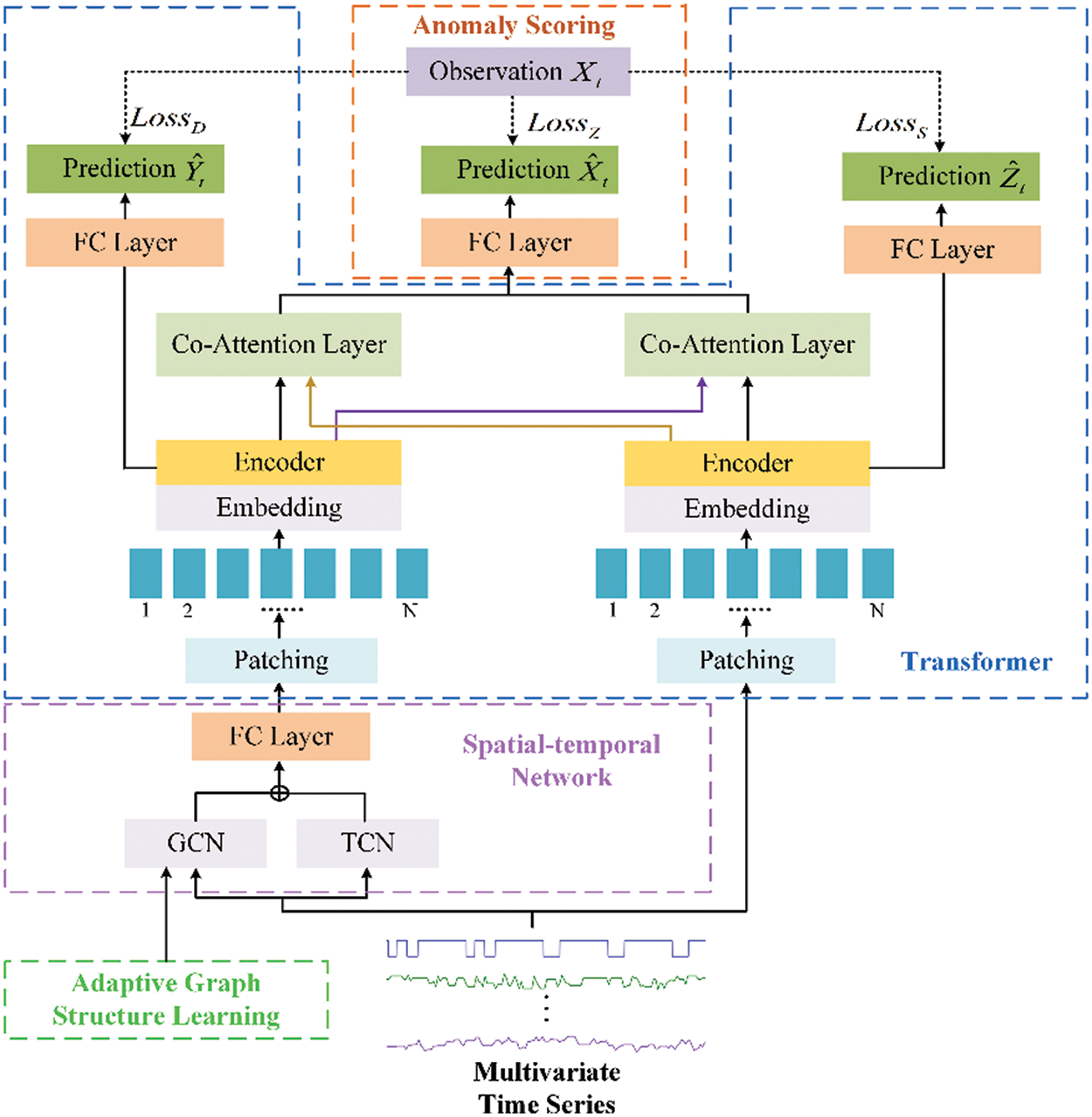
Figure 1: Overview of our proposed framework

Different from the vanilla Transformer framework, the model uses multi-head attention to encode the output of the deep network (from the spatial-temporal network), while also using multi-head attention to encode the shallow network (from the input). The shallow network mainly focuses on the basic features of the time series, and cannot fully extract and combine complex feature information. In contrast, the deep network is capable of capturing more complex relationships and higher-level features in the input data. During decoding, since anomaly detection requires consideration of both local and global information, the outputs of the shallow network and deep network are input into the cross-attention mechanism separately in the decoding stage. This ensures that the model pays attention to global information while not neglecting important local details, leading to better feature fusion and thus improving the accuracy of the model.

3.3 Spatial-Temporal Network

In IIoT, the state of a time series at a certain moment is not only related to the state of the current node over the period before (temporal correlation) but also related to the states of other nodes (spatial correlation). For example, in the wastewater treatment scenario, the water level transmitter of a tank is affected by the state of the previous period and is also influenced by other sensors such as switches and flow indicators.

As indicated in Fig. 2, we make use of a spatial-temporal network to study the relationships of time series in both time and space dimensions. Specifically, we utilize a temporal convolutional network (TCN) to identify temporal dependencies and a graph convolutional network (GCN) to identify spatial dependencies. The outputs of GCN and TCN are then aggregated and input into the next module. The introductions of GCN and TCN are as follows.

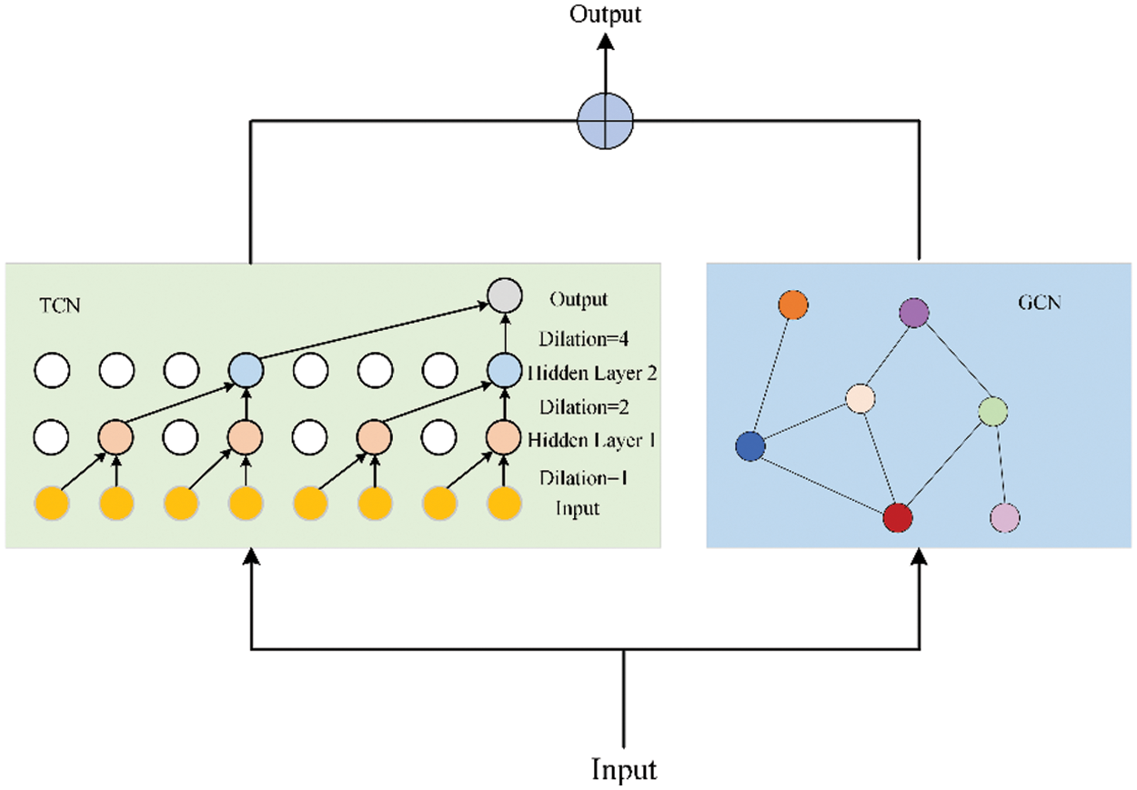
Figure 2: The spatial-temporal network architecture composed of TCN and GCN

3.3.1 Temporal Convolution Network

We employ the dilated causal convolution to obtain the temporal correlation of time series. By exponentially increasing the receptive field, dilated causal convolution can capture features from longer historical sequences with fewer layers. For the input Xi=[x1,i,x2,i,⋅⋅⋅,xL,i] of sensor i and the convolution kernel d:{0,1,…,k−1}, the dilated causal convolution operations F can be formulated as:

F(xj,i)=∑s=0k−1d(s)∗xj−r∗s,i,(2)

where k is the kernel size, r is the dilation factor, and j−r∗s is the index for the data being operated on.

3.3.2 Graph Convolutional Network

We utilize GCN to obtain the dependency relationship between the states of each sensor. To improve efficiency, the Chebyshev polynomial is used for graph convolution operation. The specific formula is displayed below:

Hl+1=σ(∑k=0K−1ΘlTk(A^)Hl),(3)

where Θl is the learnable parameters, σ is the activation function. The recursion of the Chebyshev polynomials Tk(x) denoted as Tk(x)=2xTk−1(x)−Tk−2(x), with T0(x)=1 and T1(x)=x. A^ is the normalized adjacent matrix, A^=D~−12A~D~−12, D~ is diagonal matrix, D~ii=∑jA~ij, A~=A+I, Hl is the hidden features of l layer. Since the state dependence between sensors is unidirectional, we process information by employing the following formula:

Hl+1=concat[σ(∑k=0K−1ΘPlTk(A^)Hl),σ(∑k=0K−1ΘQlTk(A^T)Hl)],(4)

where A^T is the transpose of A^, ΘPl and ΘQl are the learnable parameters, concat is the concatenation of different data.

The time complexity of temporal convolution is O(LT⋅CT_in⋅CT_out⋅kT)=O(n), where LT is the length of the input data, Cin is the number of input channels, Cout is the number of output channels, k is the size of the convolutional kernel. The time complexity of graph convolution is O(kG⋅(nG⋅cG_in⋅cG_out+mG⋅cG_out))=O(n2), where kG is the order of the convolutional kernel, cG_in is the dimension of the input features, cG_out is the dimension of the output features, nG is the number of nodes in the graph, mG is the number of edges in the graph. Therefore, the time complexity of spatiotemporal convolution is O(n2).

It should be noted that the graph adjacency matrix A employed in GCN is acquired through the adaptive graph learning method. It will be introduced in Section 3.6.

3.4 Transformer

The proposed model utilizes an improved Transformer to further learn the features within the time series. The Transformer module consists of two parts: the encoder and the decoder. Specifically, the output of the spatial-temporal network and the input time series are first sliced, and then the encoder achieves the encoding of the data and captures the interdependencies among all positions in the input sequence. This allows for a better understanding of the semantics and structural information of the input sequence. We achieve the learning of deep network features by encoding the output of the spatial-temporal network, as deep networks can capture global information. By encoding the input, we enable the shallow network to learn time series features, allowing the shallow network to capture more local features. In the decoding stage, the outputs of the shallow network and the deep network are decoded using cross-attention respectively, and then the decoded time series are sent to the next module for further processing. The following is an introduction to the encoder and decoder.

3.4.1 Encoder

The encoder module encodes the output of the spatial-temporal network and the input time series separately. The encoder structure is shown in Fig. 3.

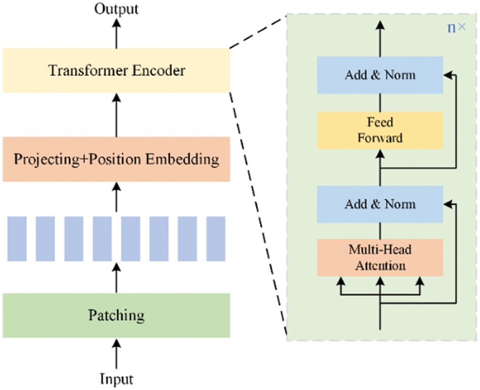
Figure 3: The structure of the patching Transformer encoder

The time series is first sliced in the time dimension. The patches can be either non-overlapped or overlapped. For input time series X int=[Xt−L,Xt−L+1,⋅⋅⋅,Xt−1], we can get XPk=[X 1k,X 2k,⋅⋅⋅,X Pk],Xik∈RP×N, 0<k≤w, where P represents the length of the patch, L denotes the length of the input time series, w=⌊L−PS⌋+1, S is the stride. Then the patches are linearly mapped to a d-dimension latent space and position embeddings are added to obtain representations X∈Rw×d. After that, the multi-head attention maps them into higher-dimensional spaces Q∈Rw×dk (queries), K∈Rw×dk (keys), and V∈Rw×dv (values), then the attention is calculated using the following formula:

Atten=Softmax(QenKenTdk)Ven.(5)

This module also includes feedforward networks, normalization layers, and residual connection networks, as shown in Fig. 3.

3.4.2 Decoder

In the decoder module, cross-attention is used to decode the encoding of the input time series and the encoding of the spatio-temporal network. Specifically, two cross-attention layers are used for decoding respectively. The Q, K, and V in cross-attention are derived from linear transformations of different inputs. Decoding is performed through the following formula:

Attde=Softmax(QdeKdeTdk)Vde,(6)

where Attde_d represents the decoding of the deep network, and Attde_s represents the decoding of the shallow network.

The time complexity of the Transformer is O(w2⋅dk+w2⋅dv)=O(n2), where w represents the length of patches, dk represents the dimensionality of Q (queries), and dv represents the dimensionality of V (values).

To ensure the effectiveness of the encoder, we input the result of the encoder into a fully connected (FC) layer to get the prediction and calculate the corresponding loss function. The specific formula is as follows:

Y^t=fθ1(Atten_dt),(7)

Z^t=fθ2(Atten_st),(8)

LossD=1T−L∑t=L+1T‖Y^t−Xt‖,(9)

LossS=1T−L∑t=L+1T‖Z^t−Xt‖,(10)

where Atten_d and Atten_s denote the coding of the deep network and the coding of the shallow network, respectively. fθ1 and fθ2 are FC layers, Y^t is the prediction of deep networks, Z^t is the prediction of shallow networks, LossD is the loss function for the deep network prediction, and LossS is the loss function for the shallow network prediction.

3.5 Anomaly Scoring

After the encoding and decoding of the Transformer, the decoded results are input into a FC layer to obtain the final time series prediction results:

X^t=fθ3(concat(Atttd,Attts)),(11)

where fθ3 is a FC layer, concat represents the concatenation of the outputs from the deep and shallow networks, X^t is the final time series prediction result. We calculate the loss function between the observation and the prediction to achieve model optimization:

LossZ=1T−L∑t=L+1T‖X^t−Xt‖.(12)

The overall loss function of our method includes the loss of the final prediction, the loss of the prediction from the deep network, and the loss of the prediction from the shallow network, as follows:

Losstotal=λLD+τLS+κLZ,(13)

where λ, τ and κ are hyperparameters.

To accurately detect anomalies and give a reasonable explanation, we calculate the difference between the observation and the prediction of each sensor. The calculation formula is given as follows:

Erri(t)=|Xt,i−X^t,i|.(14)

The maximum value at each time point is chosen as the anomaly score. The threshold is obtained through grid search [37]. When an anomaly score exceeds the threshold, it is determined that the time point is anomalous.

3.6 Adaptive Graph Structure Learning

To get better GCN results, we study the adaptive graph learning method to learn the correlation between sensors. This method consists of model training and graph learning. The model training and graph learning are implemented separately, as shown in Fig. 4. The specific process is presented as follows.

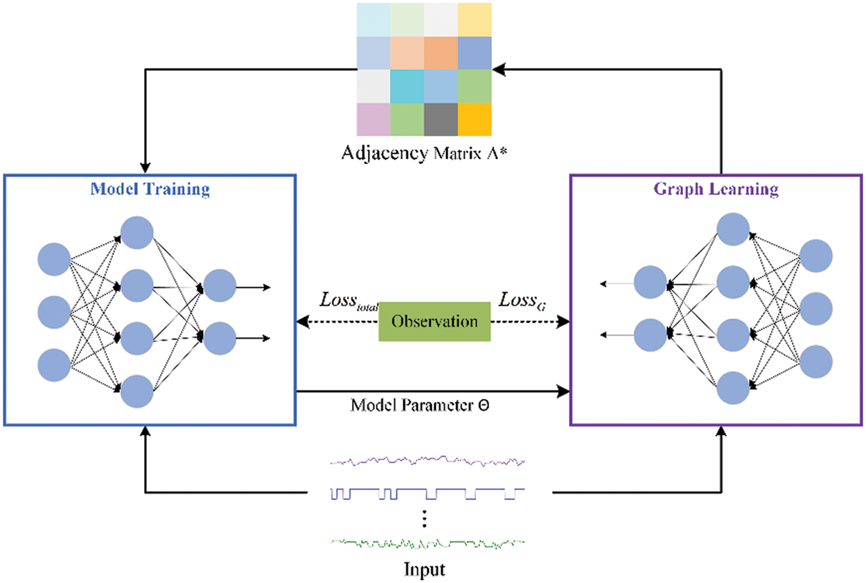
Figure 4: The process of adaptive graph structure learning

3.6.1 Model Training

Model training is used to train the proposed method, and we initialize the relation matrix A and then input it to GCN. The initialization formula for A is shown as follows:

A∗=D~−12A~D~−12,(15)

where D~ii=∑jA~ij, A~=A+I. A∗ is fixed during model training. A can be randomly generated or predefined. Unlike the method proposed in [39,40] for adaptively learning the graph adjacency matrix through the embedding matrix, we employ a random generation or expert-defined approach to obtain the initial adjacency matrix, which allows for a better representation of the asymmetric spatial correlation between sensors. In the next iteration, A is the best adjacent matrix produced by graph learning.

3.6.2 Graph Learning

For graph learning, we employ the optimal parameters Θ obtained by model training, the best adjacent matrix A∗ is obtained through training. To train the graph structure, the model parameters Θ are fixed. The new adjacent matrix can be represented as:

A2=ReLU(A1+A∗+Diag(Λ)),(16)

A3=ReLU(D~−12A~D~−12−ε),(17)

where A1∈RN∗N and Λ∈RN are the learned parameters, A∗ is from model training, D~ii=∑jA~ij, ε∈(0,1) is utilized to remove weak relations from the matrix A2.

To get the optimal matrix, push the learned adjacent matrix A3 into the matrix list adj_list. The length of the list M is a hyperparameter. We calculate the loss of each adjacent matrix to form a list l→=(L1,L2,…,LN), Lmax is the maximum value in the list, only M minimal losses are retained, and the optimal A∗∗ for model training is obtained by the following equations:

w=softmax(Lmax−l→),(18)

A∗∗=∑i=1NwiAi,(19)

where A∗∗ is the weighted sum of each adjacency matrix, w is the weight in the adjacency matrix list.

In the training of graph learning, we utilize the loss function to guarantee that the adjacency matrix is sparse:

ΔA=ReLU[ℐ(A∗∗)−ℐ(A∗)],(20)

LossG=Losstotal+ReLU(∑i=1N∑j=1NΔA(i,j)N2−δ)/δ,(21)

ℐ(x)={1 if x≠00 else ,(22)

where δ∈(0,1) is a hyperparameter that controls the sparsity of A∗∗.

Then, A∗∗ is sent into the model training as the optimal adjacency matrix, represented as A during the model training. After m epochs of training, the optimal adjacency matrix A and model parameters Θ can be obtained.

4  Experiments

4.1 Datasets

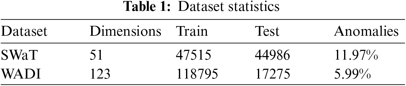
Since obtaining datasets with anomaly labels from industrial internet of things is very difficult, we use two datasets, SWaT and WADI, from the water treatment testbed designed by the iTrust research center, which are the same datasets used by other time series anomaly detection methods. The datasets simulate the normal operation of the actual water treatment system. The attack scenarios are launched by the attacker via physical elements or networks against sensors or actuators connected to the controllers (PLCs) or the SCADA system. SWaT consists of six phases with 51 sensors and actuators, which collected values from 11 days of operations, including 7 days of normal operations and 41 attack scenarios over 4 days. WADI includes 123 sensors and actuators, and it is more complex than SWaT. WADI collected sensor and actuator values for 16 days, including 14 days of normal operations and 2 days of attack scenarios. Table 1 summarizes these two datasets, the training set is Train, the testing set is Test, and the abnormal rate is Anomalies. These data are real-time records of sensor status, exhibiting significant temporal and spatial characteristics. In the temporal dimension, the current state of a sensor is closely linked to its previous states over a period of time, reflecting the time dependency of the data. In the spatial dimension, the state change of one sensor affects other associated sensors. For instance, when the switch of a water tank is turned on, the status of the water flow and water level sensors change accordingly, demonstrating the spatial dependency of the data. The experimental data are collected in seconds, resulting in a large dataset due to the small time intervals. Additionally, the changes in data over different time intervals are minimal. When evaluating time series anomaly detection methods, many studies, such as [14] and [37], use downsampling techniques to accelerate training, sampling the original data every 10 s. Therefore, in our experiments, we adopt the same method to process the data.

4.2 Experimental Setup

4.2.1 Evaluation Metrics

Precision (Pre), Recall (Rec), and F1-score (F1) are used as evaluation metrics. They are formulated as:

Pre=TPTP+FP,(23)

Rec=TPTP+FN,(24)

F1=2×Pre×RecPre+Rec,(25)

where TP is true positive (the normal time series is predicted as normal), FN is false negative (the normal time series is predicted as abnormal), and FP is false positive (the abnormal time series is predicted as normal).

4.2.2 Baselines

To illustrate the competence of our approach, we compared 10 multivariate time series anomaly detection methods. PCA [18] maps data into a lower-dimensional space through principal component analysis and determines anomalies based on reconstruction error. AE [41] consists of an encoder and a decoder, and the anomaly score is obtained by comparing the reconstructed data with the original data. DAGMM [4] incorporates both AE and Gaussian Mixture Model, and determines anomalies through density estimation in the latent space. LSTM-VAE [9] combines LSTM and VAE, with the anomaly score being the reconstruction error of the data. MAD-GAN [7] utilizes the adversarial training mechanism of GAN to learn the distribution of normal data and then identifies anomalies based on the deviation of the reconstructed data. GDN [14] introduces GAT into anomaly detection and estimates anomalies based on the degree of discrepancy between predictions and observations. GRN [16] employs GAT and GRU to learn the latent representations of time series. OmniAnomaly [8] combines GRU and VAE, uses recurrent neural networks to learn features of time series, and employs reconstruction probabilities to identify anomalies. USAD [30] constructs an AE model with two encoders and optimizes the model through adversarial training. TranAD [11] is a model based on Transformers that determines anomalies by considering the long-range dependencies in the data.

4.2.3 Training Settings

The experiments are implemented on NVIDIA 2080Ti. The model training is implemented in Pytorch 1.7.0, and we employed Adam as the optimization technique, achieving a learning rate of 0.001. The patches of SWaT and WADI are 8 and 4, the sliding window size is 64, and the number of network layers of GCN is 2.

4.3 Experimental Results

In Table 2, we show the anomaly detection performance (Precision, Recall, and F1-score) of our approach and baselines on both SWaT and WADI.

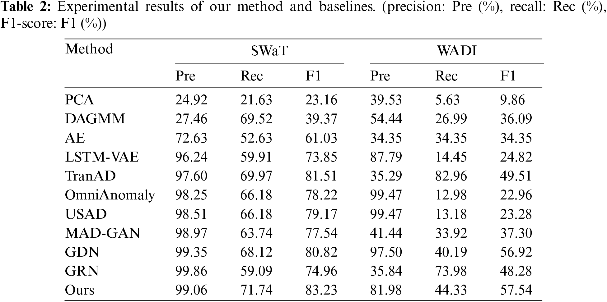
Traditional methods PCA and DAGMM perform worse than the methods based on deep learning because they have difficulty in learning nonlinear features, especially on high-dimensional datasets. Deep learning methods (AE, USAD, LSTM-VAE, OmniAnomaly, and MAD-GAN) have achieved good results in anomaly detection, but they are worse than GDN, GRN, and TranAD. GDN and GRN employ GAT to learn valid information from time series, while TranAD utilizes Transformer to learn the non-sequential sequence features of the data.

The results show that our method achieves optimal F1-score on both datasets, with SWaT achieving a 1.72% improvement compared to TranAD and WADI improving by 0.62% compared to GDN. The best recall is achieved on SWaT, WADI is second only to TranAD, and the precision of TranAD (35.29%) is significantly lower than our method on the same dataset. With the increase in data dimensions, our method may not be able to learn the characteristics of normal data well, resulting in relatively low precision. However, despite the higher precision of other models, their overall performance may be unsatisfactory. The experiment results indicate that our method has better performance outcomes than GDN and TranAD. It may be because GDN only considers spatial relationships without considering temporal relationships, while TransAD only uses self-attention without considering the correlation between spatial and temporal. This shows the feasibility of using GCN and TCN to extract time and space information of time series respectively and using an improved Transformer to learn time series features for anomaly detection.

In anomaly detection, there is an inevitable compromise between false positives (FPs) and false negatives (FNs), and it is crucial to maintain heightened sensitivity to anomalies to prevent the oversight of exceptional events, as these anomalies can potentially lead to system failures. We hold the opinion that our method achieves the best performance. Our approach achieves high F1 and recall rates as well as slightly reduced precision, but has significant implications for IIoT security.

4.4 Effect of Parameters

In this section, we explore the influence of various key parameters on the model, as illustrated in Figs. 5 and 6.

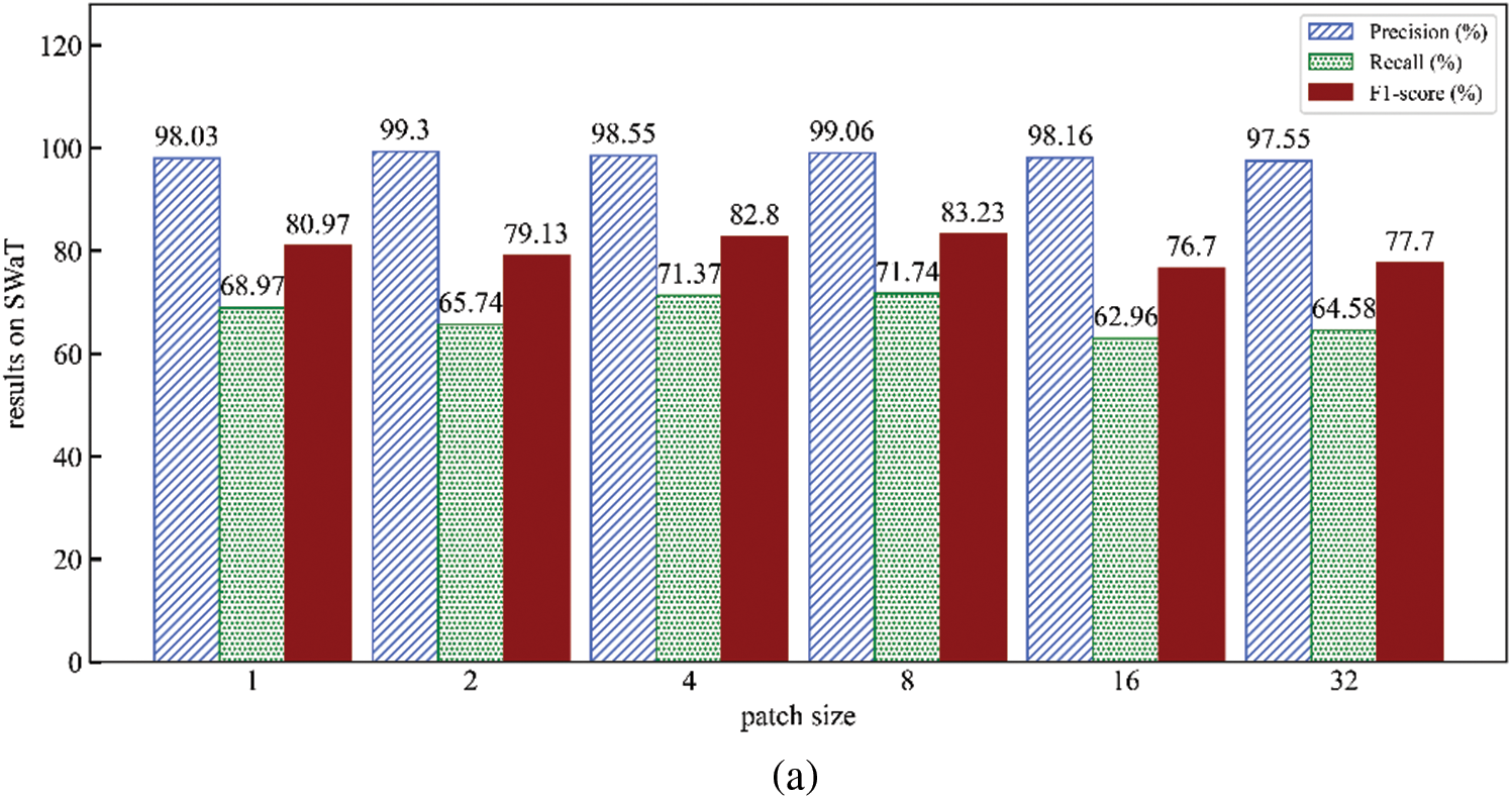
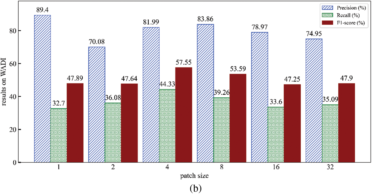
Figure 5: Effect of patch size (Results on SWaT (a) and WADI (b))

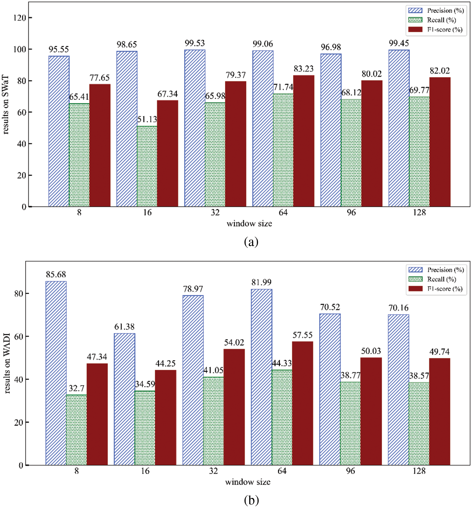
Figure 6: Effect of window size (Results on SWaT (a) and WADI (b))

4.4.1 The Impact of Patch Size

Firstly, investigate the impact of different patch sizes on the method. When P is 1, the effect is not very satisfactory. On WADI, when the batch size is set as 1, although the precision is relatively high, the performance of F1 and recall is not satisfactory. On SWaT, when the patch size P is set as 4 and 8, our method can get better results. With the increase of the patch size, the performance is improved, but the effect will decrease when the size is too large. Better results can be obtained when the patch size is 4 and 8. Therefore, patching can enhance the local semantic information and improve the performance of our method.

4.4.2 The Impact of Window Size

Then, we examine the influence of window size L on the method. L∈[8,16,32,64,96,128]. On SWaT, all L can achieve good experimental results, and the optimal result is obtained when the window is set as 64. As the window size increases, more historical information is considered in this model, and the cost of operation also increases. On WADI, window size L has a significant impact on the result. When L=8, the precision is optimal, but other performance metrics are not favorable. Good anomaly detection results can be achieved when L is set as 32 and 64. When the window is too small, it will be unable to obtain enough observation information for anomaly analysis. When the window is too large, it will increase the computational cost.

4.5 Ablation Study

To evaluate the rationality and effectiveness of the proposed method, two ablation strategies are designed. Firstly, some main modules of the model are removed or replaced to study the rationality of the method. Secondly, the performance of the method is evaluated by removing some minor components.

Firstly, remove or replace some of the main modules of the model, as illustrated in Table 3.

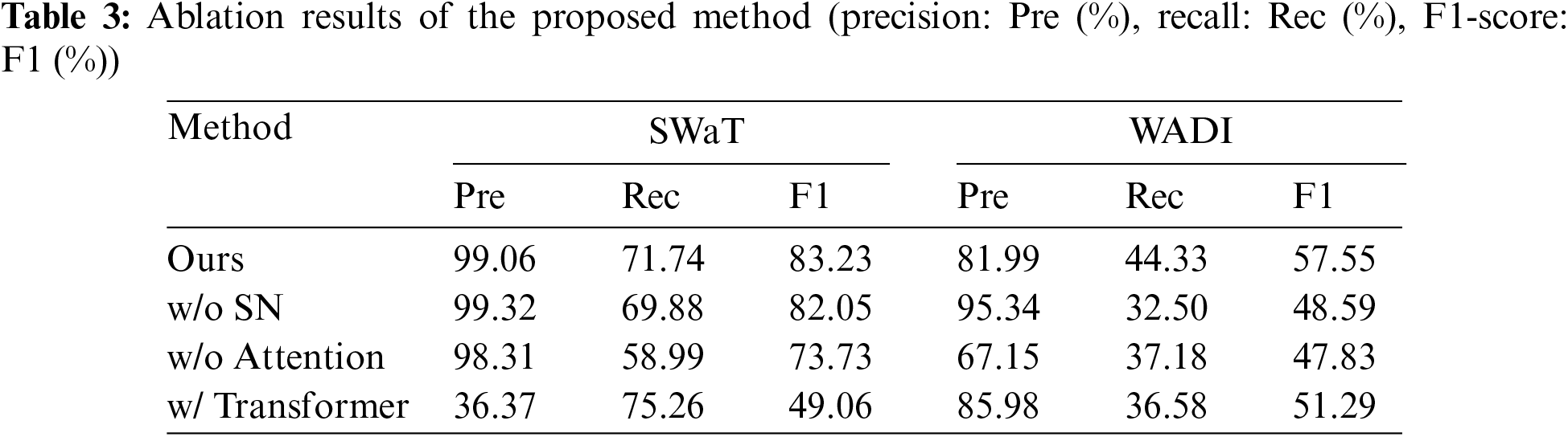
(1) w/o SN: When removing the shallow network of the model, only calculating the encoding and decoding from the spatial-temporal network, the F1-score on SWaT decreases by 1.18%, and on WADI decreases by 8.96%. Although the model is simpler, it only considers global information and neglects local information, leading to a decrease in performance. The proposed model focuses on both global information and local details through encoding and decoding of deep and shallow networks, thereby improving the accuracy of the model.

(2) w/o Attention: When the proposed model does not use the Transformer and merely relies on the spatial-temporal network to obtain features for anomaly detection, the performance of the model is not satisfactory. This may be because the features obtained by the spatial-temporal network require deeper networks for decoding, especially for high-dimensional datasets (WADI). Our model uses an improved Transformer to further learn the characteristics of the data, which improves the performance of the model.

(3) w/ Transformer: When replacing the improved Transformer with the vanilla Transformer for learning time series features, a noticeable degradation in model performance can be observed, especially on the SWaT dataset where the performance is even worse. In the proposed model, using the vanilla Transformer can effectively learn features on high-dimensional datasets, but it struggles to capture the relationships between data in low-dimensional datasets. The proposed improved Transformer utilizes patching as well as encoding and decoding with deep and shallow networks, which can better learn features of both high-dimensional and low-dimensional data, demonstrating the efficacy of our proposed method.

Then, remove some minor components from the model to evaluate its performance, as shown in Fig. 7.

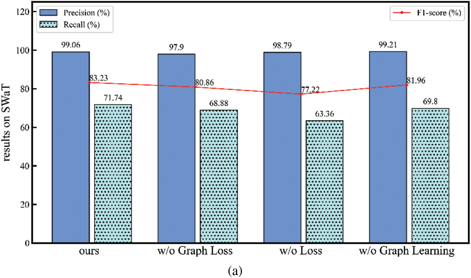
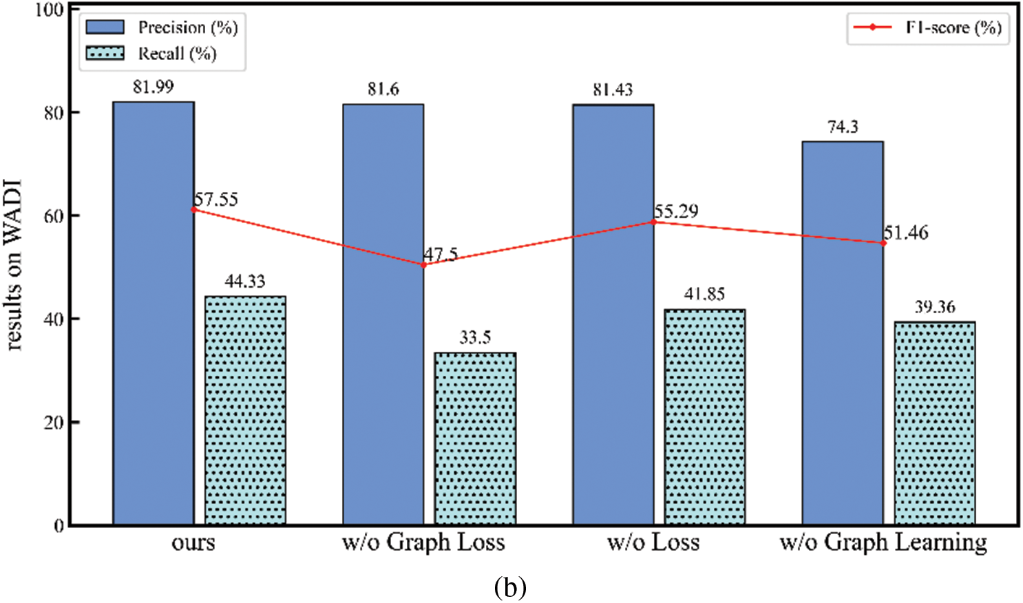
Figure 7: The anomaly detection results of the proposed method and its variants on SWaT (a) and WADI (b)

(1) w/o Graph Loss: When removing the graph loss LossG, the performance of the model will decline. On SWaT, the impact is not very significant, because SWaT has fewer dimensions. The graph loss is utilized to limit graph learning and ensure the sparsity of the graph, indicating that graph loss plays a certain role in updating the model.

(2) w/o Loss: When LossD and LossS are removed, the performance of the model will decrease. This indicates that the losses can supervise the feature learning of both the deep and shallow networks in the model, thereby ensuring the overall performance.

(3) w/o Graph Learning: When the model and graph structure are trained simultaneously, the results are not satisfactory. This indicates that performing graph structure learning and model training concurrently may lead to insufficient model training, preventing the achievement of the best possible model outcomes.

By removing some of the components from our method, we observed a change in the performance of the model, and by analyzing it we found that each component was necessary for our method.

4.6 Case Study

To further demonstrate the efficacy of the method and to intuitively describe the process of anomaly judgments, we perform case studies on SWaT and WADI. Fig. 8 shows the adjacency matrices obtained through adaptive graph learning. Figs. 9 and 10 display the true and predicted values of some sensors on SWaT and WADI. The pink blocks (ground truth) represent the labels of the test dataset, indicating that the point of time is anomalous (the system is under attack).

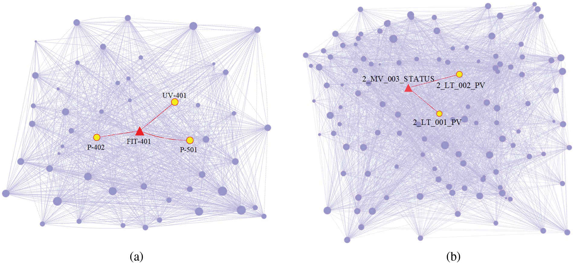
Figure 8: Undirected graph generated by graph structure learning (SWaT (a) and WADI (b))

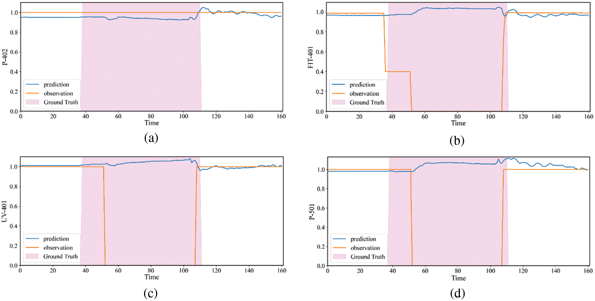
Figure 9: The true value, predicted value of P-402, FIT-401, UV-401 and P-501 on SWaT. (a) The results of P-402. (b) The results of FIT-401. (c) The results of UV-401. (d) The results of P-501. The attack period is shaded in a pink block

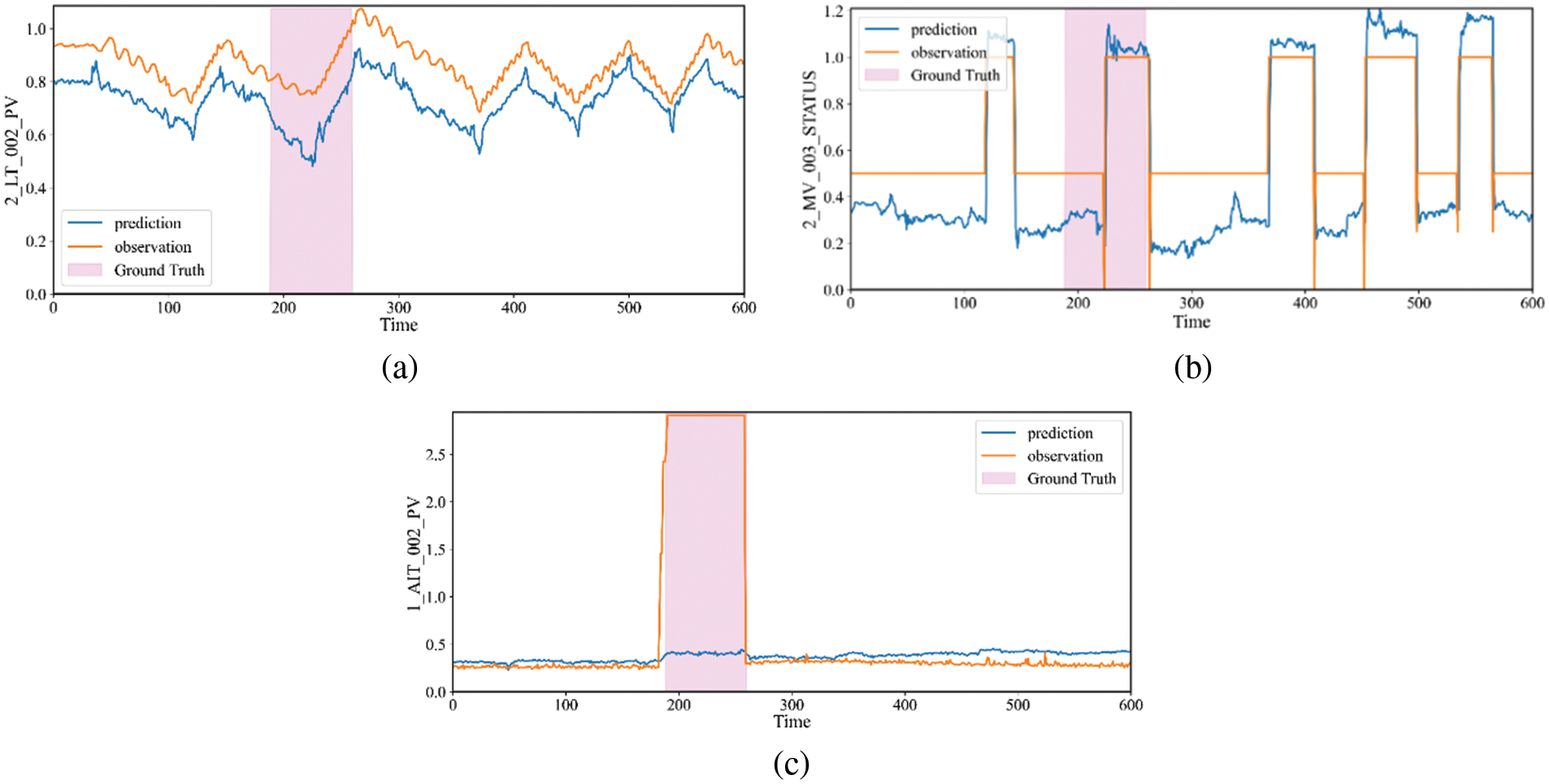
Figure 10: The true value and predicted value of 2_LT_002_PV, 2_MV_003_STATUS and 1_AIT_002_PV on WADI. (a) The results of 2_LT_002_PV. (b) The results of 2_MV_003_STATUS. (c) The results of 1_AIT_002_PV. The attack period is shaded in a pink block

4.6.1 Anomaly Case about SWaT

In reality, P-402 is the reverse osmosis supply pump, and the process of water supply is monitored by FIT-401. Then it is dechlorinated by UV-401 (ultraviolet lamps) also sent to the next stage by the P-501 (reverse osmosis pump), they are correlation. Fig. 8a is the adjacency matrix obtained by the adaptive graph structure learning, as shown in the figure, there is a correlation between FIT-401 and P-402, UV-401, P-501. It shows that our method can obtain the correct relationship between sensors. As shown in Fig. 9, in the real scenario, FIT-401 should be greater than 1. The attacker sets the value lower than 0.7 and then sets it to 0. The attacker expects UV-401 to turn off while P-501 turns off, which will stop the water treatment and affect the normal operation of the water treatment. Our model predicts that the state of FIT-401 is normal by the state of P-402, and predicts that the states of UV-401 and P-501 are normal at the same time. Comparison of the predicted and actual states reveals anomalies, indicating that our method is accurate in detecting and explaining anomalies.

4.6.2 Anomaly Case about WADI

In the real scenario, the state of MV_003 will affect 2_LT_001 and 2_LT_002. As shown in Fig. 8b, we can obtain the same correlation through graph structure learning, which also shows that our framework is effective in obtaining the relationship between sensors. By setting 1_AIT_002 to 6, the attacker releases contaminated water into the raised reservoir, while 2_MV_003 is turned on to increase the amount of water in 2_LT_002 (Elevated Reservoir). As shown in Fig. 10, when 1_AIT_002 is set to 6, our model gets the output based on the current state, 2_LT_002 decreases when 2_MV_003 is closed and 2_LT_002 increases when 2_MV_003 is opened. It is hard to find the anomaly by the state of 2_MV_003 and 2_LT_002, but our model gives a different prediction for the attack point 1_AIT_002 and gets a large deviation, so we can determine the anomaly.

In conclusion, the anomaly score of each sensor obtained by the model is helpful in detecting anomalies in time, and the adjacency matrix of sensors learned by the graph helps to understand the relationship between sensors. The prediction of each sensor and the observed state of the sensor allow us to understand how to make anomaly judgments.

5  Conclusion

In this work, we introduce a method for detecting anomalies in time series that is based on spatial-temporal network and Transformer. The method learns space and time features in time series by GCN and TCN. An enhanced Transformer architecture for further learning features of time series. In the Transformer architecture, patching and decoding implementations for deep and shallow networks contribute to the enhancement of time series feature learning. Meanwhile, we propose an adaptive graph learning method to acquire the optimal model parameters and graph structure. Finally, experiments show that our model can achieve a favorable detection effect. Overall, our proposed model is suitable for anomaly detection in wastewater treatment systems. Given its performance, we believe that this model can also be widely applied to anomaly detection in other industrial scenarios or providing effective solutions to problems in those contexts.

We find that the proposed model is relatively complex and not suitable for deployment in resource-constrained environments. In the future, we consider using knowledge distillation techniques to compress the model size while maintaining performance. Additionally, the performance of the model on high-dimensional datasets still needs to be further improved. In the future, we will consider using multi-scale feature extraction to enhance the feature learning ability of the model.

Acknowledgement: The authors would like to express their gratitude to the editors and reviewers for their thorough review and valuable recommendations.

Funding Statement: This work is partly supported by the National Key Research and Development Program of China (Grant No. 2020YFB1805403), the National Natural Science Foundation of China (Grant No. 62032002), and the 111 Project (Grant No. B21049).

Author Contributions: Conceptualization: Mengmeng Zhao and Yeqing Ren; Data curation: Mengmeng Zhao; Formal analysis: Mengmeng Zhao and Haipeng Peng; Investigation: Mengmeng Zhao and Lixiang Li; Methodology: Mengmeng Zhao; Software: Mengmeng Zhao; Supervision: Haipeng Peng and Lixiang Li; Validation: Mengmeng Zhao; Writing—original draft: Mengmeng Zhao; Writing—review editing: Mengmeng Zhao, Lixiang Li and Yeqing Ren. All authors reviewed the results and approved the final version of the manuscript.

Availability of Data and Materials: The data that support the findings of this study are openly available in the Singapore University of Technology and Design at Home - iTrust (sutd.edu.sg), accessed on 10 June 2024.

Conflicts of Interest: The authors declare that they have no conflicts of interest to report regarding the present study.

References

1. R. A. Khalil, N. Saeed, M. Masood, Y. M. Fard, M. S. Alouini, and T. Y. Al-Naffouri, “Deep learning in the industrial internet of things: Potentials, challenges, and emerging applications,” IEEE Internet Things J., vol. 8, no. 14, pp. 11016–11040, Jan. 2021. doi: 10.1109/JIOT.2021.3051414. [Google Scholar] [CrossRef]

2. G. Tabella, D. Ciuonzo, N. Paltrinieri, and P. S. Rossi, “Bayesian fault detection and localization through wireless sensor networks in industrial plants,” IEEE Internet Things J., vol. 11, no. 8, pp. 13231–13246, Jan. 2024. doi: 10.1109/JIOT.2024.3359646. [Google Scholar] [CrossRef]

3. M. Sakurada and T. Yairi, “Anomaly detection using autoencoders with nonlinear dimensionality reduction,” in Proc. Mach. Learn. Sens. Data Anal. (MLSDA), Gold Coast, QLD, Australia, Dec. 2014, pp. 4–11. [Google Scholar]

4. B. Zong et al., “Deep autoencoding gaussian mixture model for unsupervised anomaly detection,” in Proc. Int. Conf. Learn. Represent. (ICLR), Vancouver, BC, Canada, Apr. 2018. [Google Scholar]

5. P. Malhotra, A. Ramakrishnan, G. Anand, L. Vig, P. Agarwal, and G. Shroff, “LSTM-based encoder-decoder for multi-sensor anomaly detection,” arXiv preprint arXiv:1607.00148, 2016. [Google Scholar]

6. D. Li, D. Chen, J. Goh, and S. K. Ng, “Anomaly detection with generative adversarial networks for multivariate time series,” arXiv preprint arXiv:1809.04758, 2018. [Google Scholar]

7. D. Li, D. Chen, B. Jin, L. Shi, J. Goh, and S. K. Ng, “MAD-GAN: Multivariate anomaly detection for time series data with generative adversarial networks,” in Proc. Int. Conf. Artif. Neural Netw. (ICANN), Munich, Germany, Sep. 2019, pp. 703–716. [Google Scholar]

8. Y. Su, Y. Zhao, C. Niu, R. Liu, W. Sun, and D. Pei, “Robust anomaly detection for multivariate time series through stochastic recurrent neural network,” in Proc. Knowl. Discov. Data Min. (KDD), Anchorage, AK, USA, Aug. 2019, pp. 2828–2837. [Google Scholar]

9. D. Park, Y. Hoshi, and C. C. Kemp, “A multimodal anomaly detector for robot-assisted feeding using an LSTM-based variational autoencoder,” IEEE Robot. Autom. Lett., vol. 3, no. 3, pp. 1544–1551, Feb. 2018. doi: 10.1109/LRA.2018.2801475. [Google Scholar] [CrossRef]

10. R. Zhang, F. Cheng, and A. Pandey, “Representation learning using a multi-branch transformer for industrial time series anomaly detection,” in Proc. KDD, 2022 Workshop Min. Learn. Time Ser.–Deep Forecast.: Models Interpret. Appl., Washington, DC, USA, 2022. [Google Scholar]

11. S. Tuli, G. Casale, and N. R. Jennings, “TranAD: Deep transformer networks for anomaly detection in multivariate time series data,” arXiv preprint arXiv:2201.07284, 2022. [Google Scholar]

12. Y. Nie, N. H. Nguyen, P. Sinthong, and J. Kalagnanam, “A time series is worth 64 words: Long-term forecasting with transformers,” arXiv preprint arXiv:2211.14730, 2022. [Google Scholar]

13. Y. Yang, C. Zhang, T. Zhou, Q. Wen, and L. Sun, “DCdetector: Dual attention contrastive representation learning for time series anomaly detection,” in Proc. Knowl. Discov. Data Min. (KDD), Long Beach, CA, USA, Aug. 2023, pp. 3033–3045. [Google Scholar]

14. A. Deng and B. Hooi, “Graph neural network-based anomaly detection in multivariate time series,” in Proc. AAAI Conf. Artif. Intell. (AAAI), Feb. 2021, pp. 4027–4035. [Google Scholar]

15. W. Chen, L. Tian, B. Chen, L. Dai, Z. Duan, and M. Zhou, “Deep variational graph convolutional recurrent network for multivariate time series anomaly detection,” in Proc. Int. Conf. Mach. Learn. (ICML), Baltimore, MD, USA, Jul. 2022, pp. 153–178. [Google Scholar]

16. C. Tang, L. Xu, B. Yang, Y. Tang, and D. Zhao, “GRU-based interpretable multivariate time series anomaly detection in industrial control system,” Comput. Secur., vol. 127, no. 2, pp. 103094, Apr. 2023. doi: 10.1016/j.cose.2023.103094. [Google Scholar] [CrossRef]

17. F. Angiulli and C. Pizzuti, “Fast outlier detection in high dimensional spaces,” in Proc. Euro. Conf. Princ. Data Min. Knowl. Discov. (ECML-PKDD), Helsinki, Finland, Aug. 2002, pp. 15–27. [Google Scholar]

18. M. -L. Shyu, S. -C. Chen, K. Sarinnapakorn, and L. Chang, “A novel anomaly detection scheme based on principal component classifier,” in Proc. IEEE Foundations New Dir. Data Min. Workshop, IEEE Press, Piscataway, NJ, USA, 2003, pp. 172–179. [Google Scholar]

19. M. M. Breunig, H.-P. Kriegel, R. T. Ng, and J. Sander, “LOF: Identifying density-based local outliers,” in Proc. Special Interest Group Manag. Data (SIGMOD), Dallas, TX, USA, May 2000, pp. 93–104. [Google Scholar]

20. W. Lu and A. A. Ghorbani, “Network anomaly detection based on wavelet analysis,” Eurasip J. Adv. Sig. Process., vol. 2009, no. 1, pp. 1–16, 2009. doi: 10.1155/2009/837601. [Google Scholar] [CrossRef]

21. K. A. Rashedi, M. T. Ismail, A. Serroukh, and S. A. Wadi, “Wavelet based detection of outliers in volatility time series models,” Comput. Mater. Contin., vol. 72, no. 2, pp. 3835–3847, Mar. 2022. doi: 10.32604/cmc.2022.026476. [Google Scholar] [CrossRef]

22. B. Schölkopf, J. C. Platt, J. Shawe-Taylor, J. Smola, and R. C. Williamson, “Estimating the support of a high-dimensional distribution,” Neural Comput., vol. 13, no. 7, pp. 1443–1471, Jul. 2001. doi: 10.1162/089976601750264965. [Google Scholar] [PubMed] [CrossRef]

23. A. H. Yaacob, I. K. Tan, S. F. Chien, and H. K. Tan, “Arima based network anomaly detection,” in Proc. Int. Conf. Commun. Softw. Netw. (ICCSN), Singapore, Mar. 2010, pp. 205–209. [Google Scholar]

24. C. Zhang et al., “A deep neural network for unsupervised anomaly detection and diagnosis in multivariate time series data,” in Proc. AAAI Conf. Artif. Intell. (AAAI), Honolulu, HI, USA, Jan. 2019, pp. 1409–1416. [Google Scholar]

25. A. Sagheer and M. Kotb, “Time series forecasting of petroleum production using deep LSTM recurrent networks,” Neurocomputing, vol. 323, no. 3, pp. 203–213, Jan. 2019. doi: 10.1016/j.neucom.2018.09.082. [Google Scholar] [CrossRef]

26. G. I. Kim, H. Yoo, H. J. Cho, and K. Chung, “Defect detection model using time series data augmentation and transformation,” Comput. Mater. Contin., vol. 78, no. 2, pp. 1713–1730, Feb. 2024. doi: 10.32604/cmc.2023.046324. [Google Scholar] [CrossRef]

27. P. Filonov, A. Lavrentyev, and A. Vorontsov, “Multivariate industrial time series with cyber-attack simulation: Fault detection using an LSTM-based predictive data model,” arXiv preprint arXiv:1612.06676, 2016. [Google Scholar]

28. K. Hundman, V. Constantinou, C. Laporte, I. Colwell, and T. Soderstrom, “Detecting spacecraft anomalies using LSTMs and nonparametric dynamic thresholding,” in Proc. Knowl. Discov. Data Min. (KDD), London, UK, Aug. 2018, pp. 387–395. [Google Scholar]

29. F. Liu et al., “Anomaly detection in quasi-periodic time series based on automatic data segmentation and attentional LSTM-CNN,” IEEE Trans. Knowl. Data Eng., vol. 34, no. 6, pp. 2626–2640, Jun. 2020. doi: 10.1109/TKDE.2020.3014806. [Google Scholar] [CrossRef]

30. J. Audibert, P. Michiardi, F. Guyard, S. Marti, and M. A. Zuluaga, “USAD: Unsupervised anomaly detection on multivariate time series,” in Proc. Knowl. Discov. Data Min. (KDD), CA, USA, Aug. 2020, pp. 3395–3404. [Google Scholar]

31. Y. Zhang, J. Wang, Y. Chen, H. Yu, and T. Qin, “Adaptive memory networks with self-supervised learning for unsupervised anomaly detection,” IEEE Trans. Knowl. Data Eng., vol. 35, no. 12, pp. 12068–12080, Dec. 2023. doi: 10.1109/TKDE.2021.3139916. [Google Scholar] [CrossRef]

32. A. Dosovitskiy et al., “An image is worth 16x16 words: Transformers for image recognition at scale,” arXiv preprint arXiv:2010.11929, 2010. [Google Scholar]

33. Z. Yang, Z. Dai, Y. Yang, J. Carbonell, R. R. Salakhutdinov and Q. V. Le, “XLNet: Generalized autoregressive pretraining for language understanding,” in Proc. Annu. Conf. Neural Inform. Process. Syst. (NIPS), Vancouver, BC, Canada, Dec. 2019, pp. 5754–5764. [Google Scholar]

34. J. Xu, H. Wu, J. Wang, and M. Long, “Anomaly transformer: Time series anomaly detection with association discrepancy,” arXiv preprint arXiv:2110.02642, 2021. [Google Scholar]

35. X. Wang, D. Pi, X. Zhang, H. Liu, and C. Guo, “Variational transformer-based anomaly detection approach for multivariate time series,” Measurement, vol. 191, no. 1, pp. 110791, Mar. 2022. doi: 10.1016/j.measurement.2022.110791. [Google Scholar] [CrossRef]

36. J. Wang, S. Shao, Y. Bai, J. Deng, and Y. Lin, “Multiscale wavelet graph autoencoder for multivariate time-series anomaly detection,” IEEE Trans. Instrum. Meas., vol. 72, pp. 1–11, Nov. 2022. doi: 10.1109/TIM.2022.3223142. [Google Scholar] [CrossRef]

37. Z. Chen, D. Chen, X. Zhang, Z. Yuan, and X. Cheng, “Learning graph structures with transformer for multivariate time-series anomaly detection in IoT,” IEEE Internet Things J., vol. 9, no. 12, pp. 9179–9189, Jul. 2021. doi: 10.1109/JIOT.2021.3100509. [Google Scholar] [CrossRef]

38. H. Zhao et al., “Multivariate time-series anomaly detection via graph attention network,” in Proc. Int. Conf. Data Min. (ICDM), Sorrento, Italy, Nov. 2020, pp. 841–850. [Google Scholar]

39. H. Darvishi, D. Ciuonzo, and P. S. Rossi, “Deep recurrent graph convolutional architecture for sensor fault detection, isolation and accommodation in digital twins,” IEEE Sens. J., vol. 23, no. 23, pp. 29877–29891, Oct. 2023. doi: 10.1109/JSEN.2023.3326096. [Google Scholar] [CrossRef]

40. J. Yang and Z. Yue, “Learning hierarchical spatial-temporal graph representations for robust multivariate industrial anomaly detection,” IEEE Trans. Ind. Inf., vol. 19, no. 6, pp. 7624–7635, Oct. 2023. doi: 10.1109/TII.2022.3216006. [Google Scholar] [CrossRef]

41. C. C. Aggarwal, “Outlier analysis,” in The Data Mining, New York, USA: Springer, 2015, vol. 1, pp. 237–263. [Google Scholar]