A Pre-Selection-Based Ant Colony System for Integrated Resources Scheduling Problem at Marine Container Terminal

1  Introduction

With the accelerated development in the world economy and trade, the importance of marine container terminals (MCT) rapidly increases due to the rise in imported and exported goods. According to the review of maritime transport by the United Nations Conference on Trade and Development (UNCTAD), the total volumes of international seaborne trade have reached 163 million twenty-foot equivalent units (TEUs) in 2022 [1]. In particular, large MCT has huge throughput. For example, the total container throughput of the Shanghai port with more than 1000 berths has reached 47.3 million TEUs in 2022 [2]. A reasonable efficient deployment schedule of existing resources and equipment of MCT leads to an improvement of efficiency in the MCT. This efficiency will in turn enhance the competitiveness and economic performance of the MCT. At the same time, it also results in lower costs and better quality of service for shipping companies.

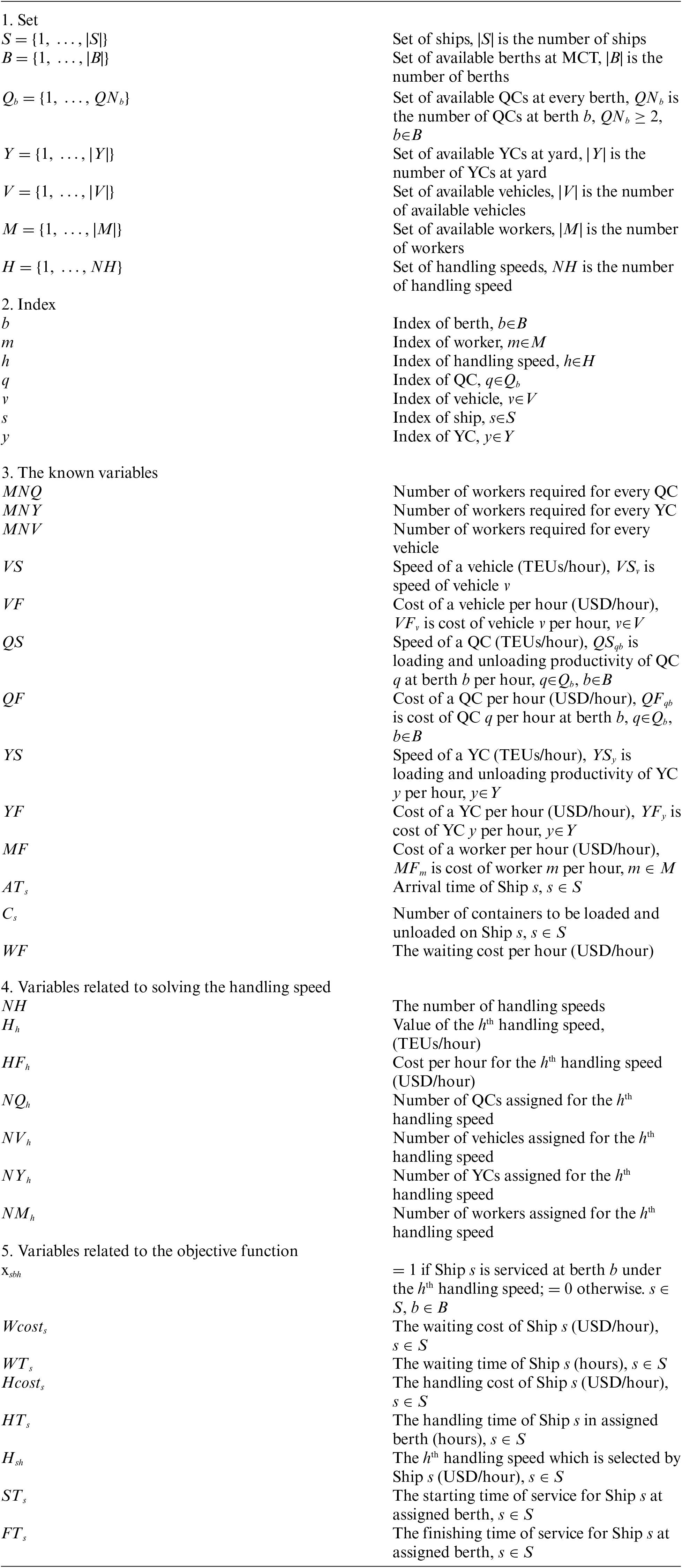
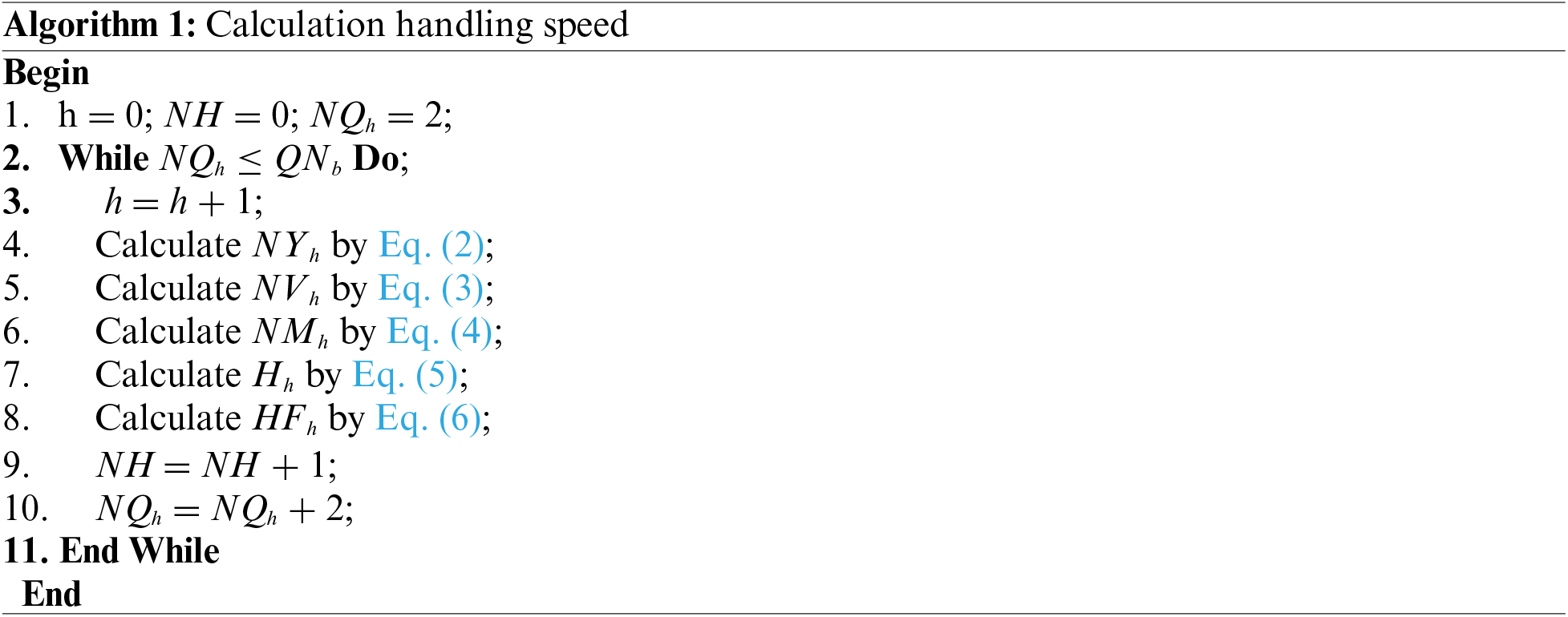
Resources of MCT mainly include berths, quay cranes (QCs), vehicles, yard cranes (YCs), and human workers. According to the container terminal layout of Qingdao port as shown in Fig. 1a, an example of the simulated resources’ layouts is shown in Fig. 1b. The workflow of each equipment resource is shown in Fig. 1c. Gray represents human resources, yellow represents transportation equipment, blue represents fixed area, and green represents loading and unloading equipment. Ship 1 is unloading containers at Berth 1 and Ship 2 is loading containers at Berth 2 in Fig. 1b. Berth provides a shoreline suitable for ship to berth and is usually divided into continuous berths or discrete berths according to the space constraint. Specifically, in the continuous berth case, the MCT is a whole shoreline and ships can berth at any position. In the discrete berth case, there are multiple berths at the MCT and only one ship can be berthed at each berth at a time. As shown in Fig. 1b, there are two discrete berths at MCT. QCs are critical equipment for loading and unloading containers from ships. There are two QCs at each berth in Fig. 1b. Vehicles transport containers between the container storage yard and the berths. YCs are lifting equipment for picking up containers from vehicles to the yard and stacking them in assigned positions in the yard, or vice versa. In Fig. 1b, two YCs are displayed to indicate their role at MCT. In non-automated MCT, human workers are essential in the supervision and operations of processes, including QCs, YCs, and vehicles [3]. Therefore, it is extremely urgent to assign these resources reasonably, which is the resources scheduling problem (RSP) at MCT.

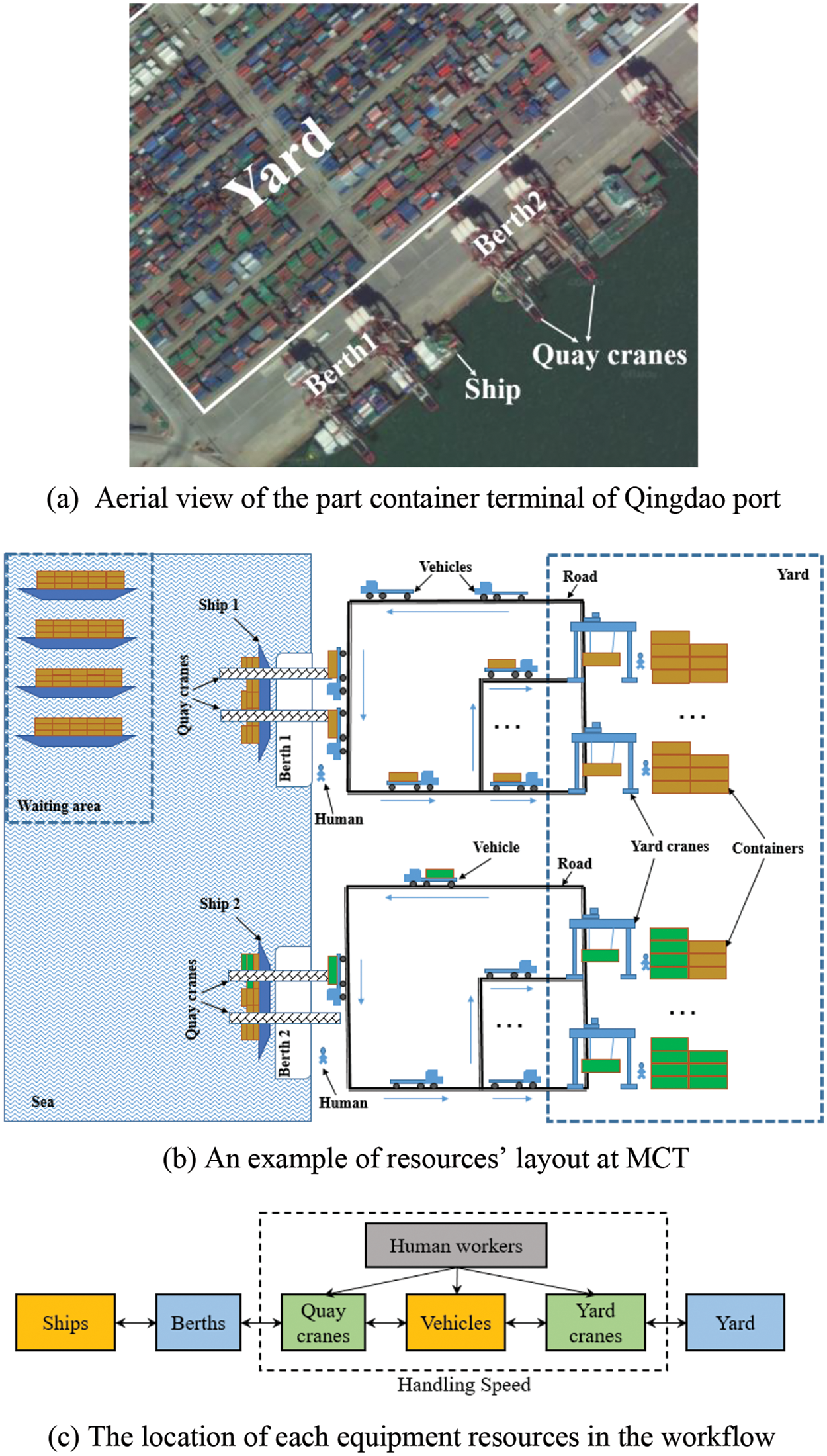
Figure 1: The loading and unloading entire process of MCT. (a) Aerial view of the part container terminal of Qingdao port (from Baidu Maps). (b) An example of resources’ layout at MCT. (c) The location of each equipment resources in the workflow

There are three main steps in the entire process of MCT operations [4] including the allocation of berths, loading or unloading containers by QCs from the ship, and picking up or putting down containers by YCs from the yard. Each resource scheduling of the RSP is included in these steps. The RSP is known as an NP-hard problem [5], and many researchers designed different strategies to solve a part problem of the RSP.

First, the available berth and berthing time are assigned to each ship that arrives at the MCT. Concerning the berth allocation problem (BAP) in RSP, many different models and algorithms have been proposed. Jauhar et al. [5] used four meta-heuristics, i.e., particle swarm optimization (PSO), advanced PSO (APSO), shuffled complex evolution (SCE), and the shuffled frog leaping algorithm (SFLA) to solve BAP for minimizing the total cost. Yin et al. [6] designed the iterative variable grouping genetic algorithm (IVGGA) for BAP to minimize the maximum berthing time of all berths. Moreover, Hameed et al. [7] solved discrete BAP by crossing the red colobuses monkey optimization with the genetic algorithm (RCMGA) to minimize the total service time. Dulebenets [8] developed a novel adaptive evolutionary algorithm (AEA) for a discrete BAP model that aims to minimize the total ship service cost. Umang et al. [9] discussed the hybrid BAP which included discrete, continuous, and hybrid berth layouts. They solved the BAP model with exact and heuristic approaches for minimizing the total service times. According to the actual conditions of MCT, where the continuous berths are always split into several discrete berthing positions, the discrete BAP is studied in our model in this paper.

Second, loading and unloading operations should be carried out. The container is unloaded or loaded from a ship by a QC in this step (i.e., QC scheduling problem), then moved to the assigned yard by a vehicle or vice versa (i.e., vehicle scheduling problem). Considering the relevance of critical equipment and resources of MCT in the terminal operations process, QCs allocation is carried out together with berths allocation. Multiple berthing positions and multiple QCs were integrated into an allocation problem model in [10], which aimed to minimize the total cost. In [11], a biased random key genetic algorithm (GA) was proposed to allocate berthing positions and assign several QCs for every incoming ship. Li et al. [12] proposed a two-phase iterative heuristic algorithm for an integrated model with continuous berth allocation and QC assignment to optimize two objectives, which minimizes total turnaround time and total penalty cost simultaneously.

Third, when the vehicle arrives yard, the container is picked up or put down from the yard by a YC (i.e., YC scheduling problem). Cao et al. [13] developed a heuristic algorithm to minimize the loading time of the containers for planning and scheduling YCs. The problem of multiple equipment assignments and scheduling at MCT has also been extensively studied. Cahyono et al. [14] presented a model predictive algorithm to solve the integrated terminal operations problem, including the allocation and scheduling of QCs, trucks, and YCs, and selecting the storage positions of containers in the yard and ship. Li et al. [15] proposed a new mixed-integer programming model with many equipment, such as QCs, automated vehicles, reach stackers, YCs, and outside container trucks in automated MCT, and also designed an improved GA to minimize total loading and unloading operation time. Tanaka et al. [16] proposed an improved branch and bound algorithm to obtain YCs and a yard scheduling plan to minimize the number of relocations. Xiang et al. [17] constructed a multi-objective dynamic integrated optimization problem model, including BAP, QC assignment problem, and yard assignment problem. Considering the human workers scheduling problem, Maione et al. [18] proposed a generalized stochastic Petri net model, which described how to coordinate humans and use resources (i.e., cranes and transporters).

Most of the aforementioned studies only study a part of the RSP. That is, scheduling only a part of the resources. However, the MCT manager needs to plan the entire operation process so that global efficiency can be obtained. Therefore, all the resources, including berths, QCs, YCs, human workers, and vehicles should be considered together and integrated. However, each part of the RSP is NP-hard, like the BAP, the QC scheduling problem, the vehicle scheduling problem, the YC scheduling problem, and the human workers scheduling problem. In this sense, the integrated RSP would be much more complex. Fortunately, all these scheduling problems share a common objective of reducing operation costs. For example, unreasonable berths allocation can lead to unreasonable waiting times for the ships, causing a higher waiting cost. Moreover, the cost also heavily relates to the handling speed of the operation in the scheduling. If more equipment or resources (i.e., QCs, YCs, human workers, and vehicles) are used, the handling speed will be faster, leading to shorter waiting time but causing a higher handling cost per unit time. Motivated by this, in this paper, we first establish a novel integrated RSP model and set the total cost minimization as the optimization objective of the integrated RSP model by combining the waiting cost and handling cost, which can consider all the resources or equipment together in the integrated RSP model.

Metaheuristic algorithms are suitable for solving NP-hard RSP-related problems, such as PSO [5], GA [19–21], and hybrid algorithm [22–26]. However, PSO may be suitable for solving continuous optimization problems in general, and its performance may degrade for discrete problems. Moreover, GA-based approaches may produce infeasible solutions in the process of crossover and mutation, which requires extra computational burden to repair. Therefore, we propose solution construction on the graphical structure to avoid generating infeasible solutions.

Ant colony system (ACS), derived from ant colony optimization (ACO), is a metaheuristic algorithm that is more effective and efficient in dealing with discrete optimization problems [27]. Currently, ACS has been used to solve various resource-constrained combinatorial optimization problems in the real world, such as traveling salesman problem (TSP) [28], supply chain configuration [29], cold chain logistics scheduling [30], virtual machine placement problem [31], path planning optimization problem [32,33], and discrete BAP [34]. These applications highlight the robustness and the ability of the global search of ACS. Inspired by ACS, in this paper, we further propose a solution construction method on the graphical structure to avoid generating infeasible solutions. Moreover, a pre-selection strategy is designed to meet the practical requirement and accelerate the convergence speed. Therefore, the complete algorithm pre-selection-based ACS (PACS) is proposed to solve the integrated RSP model for minimizing the total cost.

Based on the above, the main contributions of this paper come from both the problem model aspect and the algorithm design aspect, which are summarized as follows:

1. In the problem model aspect, different from other models that only consider scheduling part of the resources in MCT, due to the strong interrelation in the different equipment resources of MCT, we establish a novel integrated RSP model that combines multiple resources (including berths, QCs, YCs, human workers, and vehicles) together in a uniform model. This way, all the resources at the MCT can be considered together at the same abstract level and be allocated and scheduled simultaneously to minimize the total cost.

2. In the algorithm design aspect, the PACS approach is proposed based on graphic structure solution representation and a pre-selection strategy. Firstly, in order to avoid generating infeasible solutions, the graphic structure is proposed to encode the solution and the solution construction process imitates the idea of finding the shortest path method based on the graphic structure. This graphical structure can avoid the same ship node being repeatedly selected. Secondly, aiming to meet the real-time requirement of the RSP model and reduce the search space to further improve the performance, the pre-selection strategy is proposed to accelerate the optimization speed of PACS.

The rest of this paper is organized as follows. In Section 2, the integrated RSP mathematical model is given, with a detailed description of the objective function of the RSP. Section 3 describes the details of PACS for solving RSP. Experiments are carried out in Section 4, and test results are compared with other algorithms on robustness, effectiveness, and efficiency. Finally, conclusions and future work are drawn in Section 5.

2  Problem Formulation

2.1 Notations

The mathematical symbol representation and formula of the RSP model are given as follows:

2.2 Problem Description

The RSP is a problem for the unified scheduling of equipment and resources at MCT by the terminal manager. The scheduled equipment and resources include:

1. Available discrete berth B. A berth can only serve one ship at a time. All berths meet berthing conditions of all ships. Once selected, ship will not change the berth until the ship completes the operation and leaves the berth.

2. Available QCs at every berth, Qb = {1, …, QNb}. We set the same number of QCs at every berth. The number of QCs can affect the handling speed, and resulting in different costs. In actual terminal operation, to avoid increasing the weight difference between the two sides of the ship, the number of QCs is often an even number to keep the ship stable (i.e., both QNb and NQh are even numbers), so QNb ≥ 2.

3. Available YCs at every yard, Y = {1, …, |Y|}. In general, the number of YCs should not be too larger or too small. The number of YCs should generally meet the following condition:

|Y|=arg min|Y|{(∑b=1|B|(∑q=1QNbQSqb))≤YS×|Y|}(1)

Specifically, since multiple berths are corresponding to one yard area, the total handling speed of YCs needs to cope with the simultaneous operation of QCs at all berths. Meanwhile, the quantity of YCs will not exceed that of QCs too much. Otherwise, some YCs will be idle during unloading or make the QCs too busy to meet the requirements of all containers during loading. Furthermore, a YC can only serve one berth at a time.

4. Available vehicles. The number of vehicles used by per handling speed is determined by the number of QCs and YCs. Using more QCs and YCs requires more vehicles, causing higher cost. Only one operation (loading or unloading) is performed at a time. Correspondingly, each vehicle also carries out only one operation at a time. For example, the vehicle takes the container from the ship to the yard and returns to the berth empty, or loads the container from the yard to the berth with containers and returns to the yard empty. As shown in Fig. 1b, Ship 1 is unloading and Ship 2 is loading.

5. Available workers, the number of workers is sufficient. We set each equipment is operated by only one worker. The total number of workers is the number of equipment served for Ship s. Each worker cannot operate more than one device at the same time.

For a better understanding of the operation flow in the whole MCT, Fig. 1b describes an example of the layout and workflow of MCT. Ships arrive at the MCT one after another, instead of unified scheduling after all ship arrived. When ship arrived before its service time, it will wait in the waiting area. The waiting time of the Ship s (WTs) is calculated by its arrival time (ATs) and starting time of service (STs). When the waiting time of a ship is over and the ship is berthed, a handling speed is assigned to the ship. The handling speed is determined by the number of equipment allocated to the ship and the speed of each piece of equipment, shown in the dashed box in Fig. 1c. Finally, complete the transport of containers based on the allocated handling speed between the ship and yard (i.e., loading or unloading) before the ship leaves the berth.

Considering the actual situation of MCT, the assumptions can be summarized as follows: (1) Ships cannot berth at multiple berths at the same time and cannot be served at multiple handling speeds. (2) Every ship continues to work at a selected handling speed until the loading and unloading are done. (3) All the equipment keeps the same running speed.

2.3 The Handling Speed

We integrate multiple equipment-dependent parameters into one metric, called handling speed. The faster handling speed often needs more equipment (i.e., QCs, YCs, human workers, and vehicles) also brings the higher cost. Therefore, the values of each handling speed are computed according to the quantity of partially used equipment (NQh, NYh), while the costs of every handling speed HFh are calculated according to the cost of used equipment (NQh, NYh, NVh, NMh). The pseudo-code of the calculation process of handling speed is given in Algorithm 1.

The value of QNb and NQh are even numbers, so the value of NQh is set to 2, 4, …, and QNb in turn, which are shown in Line 1 and Line 10 of Algorithm 1.

Since QCs in discrete berths cannot be used in different berths, the upper limit of Hh is the sum of the speed of all QCs in a single berth. In Line 2 of Algorithm 1, NQh is no more than the number of QCs for a single berth. Due to QNb ≥ 2, we set the initial value of NQh to 2. In Line 4 of Algorithm 1, NYh (i.e., the number of YCs assigned for hth handling speed) is calculation by:

NYh=arg minNYh{YS×NYh≥QS×NQh≥YS×(NYh−1)}orarg minNYh{YS×(NYh+1)>QS×NQh}(2)

In Line 5 of Algorithm 1, the number of vehicles assigned for the hth handling speed is computed by:

NVh=arg minNVh{QS×NQh≤VS×NVh&YS×NYh≤VS×NVh}(3)

The total number of workers served for the hth handling speed is calculated in Line 6 of Algorithm 1, the calculation equation is shown as follows:

NMh=NQh+NVh+NYh(4)

Combined with the above calculation results, in Line 7 of Algorithm 1, the value of the hth handling speed is calculated by:

Hh=min{QS×NQh,YS×NYh}(5)

We compare the speed of QCs (QS × NQh) with the speed of YCs (YS × NYh), and assign the minimum value to Hh.

Then, the cost per hour of the hth handling speed is computed in Eq. (6). The cost includes the total cost of QCs, YCs, vehicles, and workers, which are allocated to the hth handling speed.

HFh=NQh×(QF+MF)+NYh×(YF+MF)+NVh×(VF+MF)(6)

The quantity of handling speed NH is counted by algorithm execution, which is shown in Line 10 of Algorithm 1.

In the proposed RSP model, the calculation of handling speed needs to meet the following constraint:

QN1=QNb,∀b∈B(7)

VS=VS1=VSv,∀v∈V(8)

VF=VF1=VFv,∀v∈V(9)

QS=QS11=QSqb,∀q∈Qb,∀b∈B(10)

QF=QF11=QFqb,∀q∈Qb,∀b∈B(11)

YS=YS1=YSy,∀y∈Y(12)

YF=YF1=YFy,∀y∈Y(13)

MF=MF1=MFm,∀m∈M(14)

MNQ=MNY=MNV=1(15)

NQh≤QNb(16)

NYh≤|Y|(17)

(∑b=1|B|QNb)≤|Y|(18)

NMh≤|M|(19)

NVh≤|V|(20)

Constraint (7) defines that the number of available QCs at every berth is same. Constraint (8) indicates that the speed of every vehicle is the same. Constraint (9) guarantees that the cost of every vehicle per hour is same. Constraint (10) states that the speed of every QC at any berth is same. Constraint (11) signifies that the cost of every QC per hour is same. Constraint (12) represents that the speed of every YC is same. Constraint (13) indicates that the cost of every YC per hour is same. Constraint (14) represents the hourly wage of every worker is same. Constraint (15) expresses only one worker is required to operate each device at a same time. Constraints (16)–(20) imply the number of QCs, YCs, and vehicles assigned for the hth handling speed are the allowable amount.

2.4 Mathematical Model of RSP

Objective:

Minimizef=∑s=1|S|(Wcosts+Hcosts)(21)

subject to:

∑b∈B∑h∈Hxsbh=1,∀s∈S(22)

STs≥ATs,∀s∈S(23)

STs={ATsFTsp≤ATsFTspFTsp>ATs(24)

WTs=STs−ATs,∀s∈S(25)

Wcosts=WTs×WF,∀s∈S(26)

HTs=Cs/Hsh,∀s∈S(27)

FTs=STs+HTs,∀s∈S(28)

Hcosts=HFh×HTs,∀s∈S(29)

Based on the components mentioned above, the objective of the integrated RSP model is to minimize the total cost, which includes waiting cost and handling cost of all ships, shown in function (21). Constraint (22) ensures that each ship must be served once at any berth. Constraint (23) ensures that the ship will not be served until it arrives. Eq. (24) calculates the staring time of service for Ship s, where sp is the previous ship that berthed at the same berth as Ship s. When the finishing time of service for Ship sp is less than ATs, Ship s will be berthed directly; otherwise, it will wait for the Ship sp to complete the operation. Eq. (25) calculates the waiting time of Ship s. Eq. (26) computes the waiting cost of Ship s. Eq. (27) calculates the handling time of Ship s. Eq. (28) computes the finishing time of service for Ship s. Eq. (29) computes the handling cost of Ship s.

3  PACS for Solving RSP

PACS is used to solve RSP, which is to find an optimal berthing scheme with the minimum cost. The objective function of RSP is defined in Eq. (21). The optimal berthing scheme includes berthing berth, handling speed, and berthing sequence of every ship.

When using PACS to solve the RSP, the solution representation should be defined. Herein, a novel graphic structure for solution representation is proposed. Based on the solution representation, the optimization process is described as follows. Firstly, the ant randomly chooses a node as the starting point. Then, the ant chooses the next node according to the biased exploration based on the pheromone and heuristic information between nodes. A complete solution path is constructed by repeating this process until all the ship berthing schemes are determined. After that, local pheromones updating rule is executed to reduce the probability of other ants choosing the same path, where the pheromone on the paths visited by the ant is weakened by the local pheromone updating rule. When all ants construct their solutions in this generation, these solutions are compared with the historically best solution to obtain a new historically best solution. The pheromone is enhanced on the edges of the new historically best solution, to accelerate the convergence speed of the algorithm. The process will be repeated until the terminal condition is met.

In the following parts, the graphic structure solution representation, initialization state configurations, state transition rule, and pheromone updating rules are described in details, with the complete PACS algorithm in the end.

3.1 Graphic Structure for Solution Representation

The RSP is similar to TSP. The goal of TSP is to find the shortest path for a traveler to go through all the cities without repetition. Therefore, RSP can also be constructed into a graphic structure similar to a city map. The goal of RSP is to find the shortest path which is an optimal berthing scheme for every ship, including berthing berth, handling speed, and berthing sequence.

The RSP can be modeled into a digraph with |S| × |B| × NH nodes. The state of each ship is represented as xsbh (s∈S,b∈B,h∈H), which means Ship s is served under handling speed h in berth b. An example of the graphic structure for RSP is shown in Fig. 2, which includes 16 nodes representing 16 states of 4 ships (|S| = 4) with 2 berths (|B| = 2) and 2 handling speeds (NH = 2). Each ship has |B| × NH state. For instance, x321 means Ship 3 is served under handling speed 1 in Berth 2. The same ship can only be chosen once, so there is no edge between nodes of the same s value denoted in every dotted line in Fig. 2a. For other nodes, there are paths between any two nodes, and there are different path distances in two directed edges between these nodes. These edges are similar to the city path in TSP. Then, the best path is calculated by the PACS algorithm. Fig. 2b shows a path that stands for an RSP scheduling scheme. Unlike the TSP, this path does not need to go back to the start node. The sequence of the path indicates the sequence in which the ship berths. The node information in the path represents the berthing berth and handling speed selected for each ship. For instance, Fig. 2b shows berthing sequence of 4 ships, which is Ship 1 at Berth 1 with 2th handling speed (x112 = 1), Ship 2 at Berth 1 with 1th handling speed (x211 = 1), Ship 3 at Berth 2 with 2th handling speed (x322 = 1), and Ship 4 at Berth 2 with 2th handling speed (x422 = 1).

Figure 2: Graphic structure for RSP. (a) All paths between ship nodes (solution space). (b) A berthing scheme (a feasible solution)

3.2 Initialization State Configurations

Initialization operation includes computing handling speed, initialing pheromones, and determining the starting node. The pre-selection strategy is proposed in initialization operation to reduce the computational burden and to fast obtain a higher quality solution.

3.2.1 Initialization of the Handling Speed

In the initialization stage of PACS algorithm, RSP determines the handling speed by considering multiple resources (QCs, YCs, human workers, and vehicles). These values of variables related to handling speed (i.e., Hh, HFh, and NH) are calculated by Algorithm 1.

The quantity of vehicles and workers are determined by the quantity of QCs and YCs, shown in Eqs. (2) and (3). The value of handling speed Hh is also determined by the number of QCs and YCs, shown in Eq. (5). Then, the corresponding cost for each handling speed is calculated by Eq. (6). The more equipment and workers used, the higher the cost per unit time. Finally, the number of handling speed NH is counted by Algorithm 1. NH is used to determine the number of nodes of RSP graph during the process of constructing RSP graph structure.

3.2.2 Initialization of Pheromones by Pre-Selection Strategy

We first proposed the pre-selection strategy based on first come first served (FCFS) to determine the initial pheromone value τ0, so as to meet the practical requirement and find the short path quickly, accelerating the convergence speed. Specifically, the FCFS algorithm is used to solve RSP and find a solution EFCFS, which includes the berthing sequence, berthing berth, and handling speed of each ship. In EFCFS, the handling speed of each ship is the lowest handling speed [24]. Then, a more suitable handling speed is calculated by the pre-selection strategy. The berthing sequence and berthing berth remain unchanged. Berthing sequence and berthing berth determine the berthing time interval between each ship. The calculation formula for new handling speed is defined as follows:

H′sh={ argminHsh{ Hcosts }argminHsh{ Hcosts+Wcosts+1 }  s∈S′′otherwise(30)

where s ∈ EFCFS, s + 1 is the ship that berths after Ship s in the EFCFS. S′′ is a set that consists of the last ship berthed at each berth. The unchanged berthing sequence, unchanged berthing berth, and new handling speed combine to form a new berthing scheme EPFCFS. Then, the fitness of EPFCFS is calculated by Eq. (21), as fPFCFS. The pheromones are initialized as τ0 = (|S| × fPFCFS)-1.

3.2.3 Initialization of the Starting Node by Pre-Selection Strategy

In this step, the pre-selection mechanism is used to determine the starting node of every ant (ant_n0) in every generation. A pre-selection parameter ξ (0 ≤ ξ ≤ 1) is introduced to initialize the starting node of every ant. All ships are sorted according to the arrival time, and the first 1/4 ships are selected by the arrival time to form a new pre-selected ship set PS. Referring to [34], 1/4 is the most suitable value to obtain a better solution at a lower computational cost. Then, starting points of every ant are selected as:

ant_n0{xsbh=1,∀s∈PS,∀b∈B,∀h∈Hif z≤ξxsbh=1,∀s∈S,∀b∈B,∀h∈Hotherwise(31)

where z (0 ≤ z ≤ 1) is a random number, and compares with ξ. If z ≤ ξ, we randomly select a note that arrives time earlier in set PS. Otherwise, any node can be chosen as the starting point. The pre-selection parameter ξ is used to balance the exploitation and exploration for constructed solution processes.

3.3 State Transition Rule

In PACS algorithm, pheromone and heuristic information are used to guide forward behavior of ants in the state transition rule. Heuristic information is introduced as follows:

η(i,j)={1/(abs(ATi−ATj))1/(2×abs(ATi−ATj)) if ATi>ATjotherwise(32)

where “abs()” is the absolute function. Heuristic information is used to guide the search behavior of ants. Ants are biased to select ship j whose arrival time is closer and earlier to the arrival time of ship i.

In PACS algorithm, each ant from node i move to the next node j in set S′ by state transition rule, where the set S′ is the unvisited node that can be selected by the ant on the current node i. The next node j is selected by following rule:

j={arg⁡maxj∈S′{[τ(i,j)]×[η(i,j)]β}if q≤q0Jotherwise(33)

where β (β > 0) is a control parameter that represents the relative importance of pheromone vs. heuristic information. q0 is a control parameter, which controls ants to choose the next nodes greedily or randomly. In Eq. (33), if random number q (0 ≤ q ≤1) meets q ≤ q0, the ant chooses the next node with maximum the heuristic information and pheromone. Otherwise, a roulette wheel selection mechanism is used to select the next node, shown as:

p(i,j)={τ(i,j)×η(i,j)β∑u∈S′τ(i,u)×η(i,u)β,if j∈S′0,otherwise(34)

3.4 Pheromone Updating Rules

In PACS algorithm, there are two kinds of pheromone updating rules, which are the local pheromone updating rule and the global pheromone updating rule. The local pheromone updating rule is used to reduce pheromones of visited edges to avoid the following ants choosing the same edges. The local pheromone is updated when each ant constructs a complete solution, shown as:

τ(i,j)=(1−ρ)×τ(i,j)+ρ×τ0(35)

where ρ is the pheromone decay parameter.

When every generation is complete, the global pheromone update is carried out on the edge of the best-so-far solution. The pheromone is increased as:

τ(i,j)=(1−ε)×τ(i,j)+ε×(fBest)−1if(i,j)∈EBest(36)

where EBest is the best-so-far solution, fBest is the fitness of best-so-far solution, and ε is the pheromone enhancement parameter.

These two pheromone updating rules act in different roles and complement with each other. The local update is more beneficial to expand the selection direction of ants. The global pheromone updating rule makes ants gradually converge to the best solution and speeds up the convergence of the algorithm.

3.5 Complete PACS Algorithm

The complete PACS algorithm is shown in Fig. 3 and the details are described as follows:

Step 1: Initialize the handling speed and the pheromone, shown in the sub-flowchart on the right side of Fig. 3. Specifically, calculate the handling speed and build the RSP model. Then, a solution EFCFS is constructed by FCFS algorithm. After that, calculate the appropriate handling speed by pre-selection strategy for every ship and get a new solution EPFCFS. Finally, evaluate the fitness fPFCFS by (21) and obtain the initial pheromone τ0.

Step 2: Set the first ship by pre-selection strategy for ant.

Step 3: Construct the whole solution by state transition rule as (33) and (34). Then, the local pheromone is updated by (35).

Step 4: When all ants find the solution in the current generation, we calculate a more appropriate handling speed for the current optimal solution, similar to Step 1, and obtain a new optimal solution.

Step 5: Perform the global pheromone updating as (36). Otherwise, go to Step 2.

Step 6: Termination check. If the maximal generations NG is reached, the process terminates. Otherwise, move to Step 2 and continue optimizing until termination condition is met.

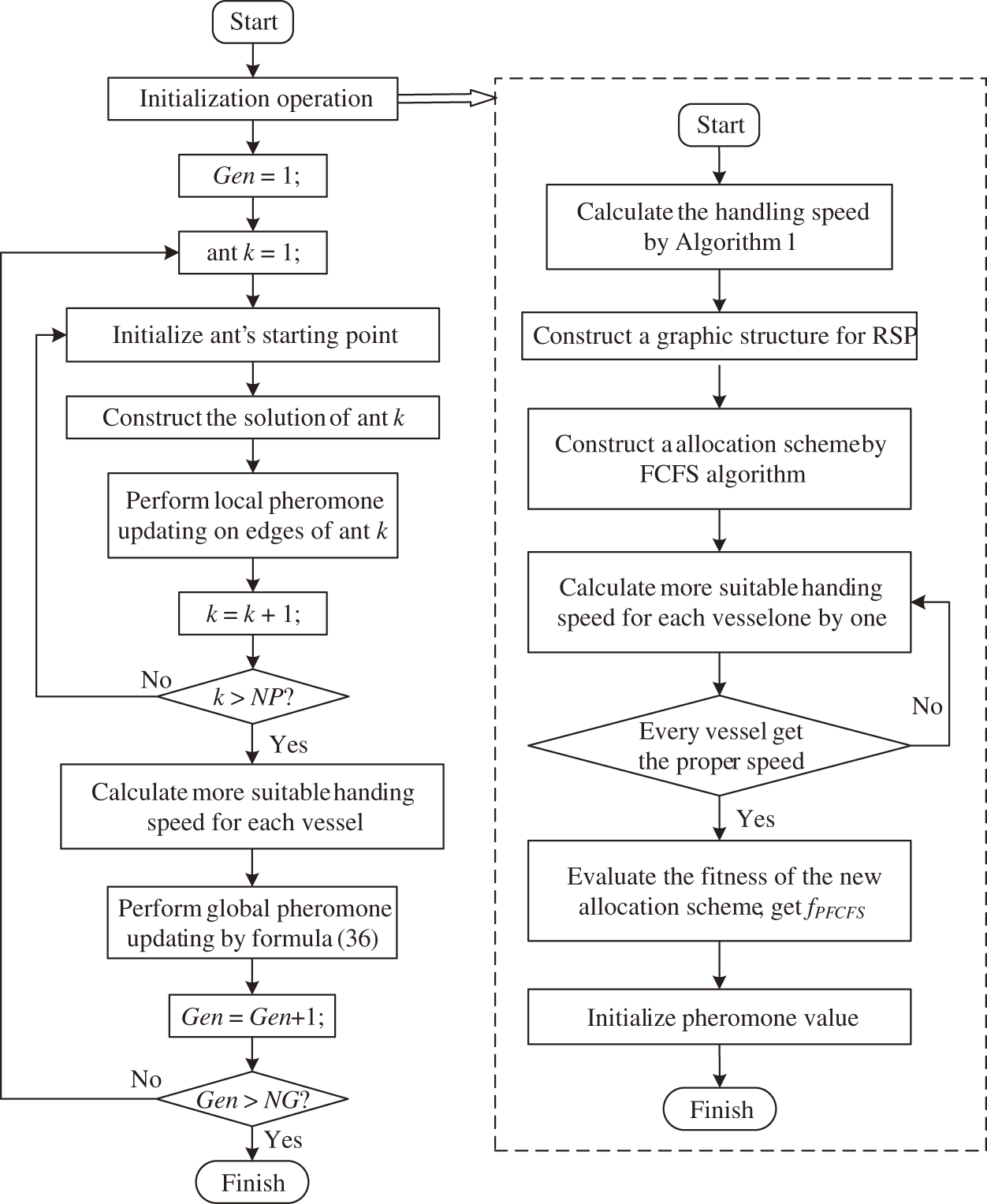
Figure 3: Flowchart of the PACS algorithm

3.6 Complexity Analysis

According to the complete PACS algorithm shown in Fig. 3, we first need to initialize the handling speed, the time complexity is O(NH), where NH is the number of handling speeds. Then, we should construct the whole solution of an ant, the time complexity is O(AA), where AA is the number of nodes that each ant needs to access. After that, we should find the solution for all ants, the time complexity is O(NP × AA), where NP is the number of ants. Next, we should evaluate the solution and perform the global pheromone updating with the time complexity O(AA−1). The process will be repeated NG times, where NG is the maximal generations. Therefore, the complete time complexity of PACS is O(NG × NP × AA).

4  Experiments and Comparisons

In this section, we conducted experiments with different sizes of tests to verify the performance of PACS. The code of the PACS algorithm is implemented in Visual C++ on a PC with Dell Intel(R) Core-i7 and 8.0 GB RAM.

4.1 Parameters and Data Description

4.1.1 Initialization of the Handling Speed

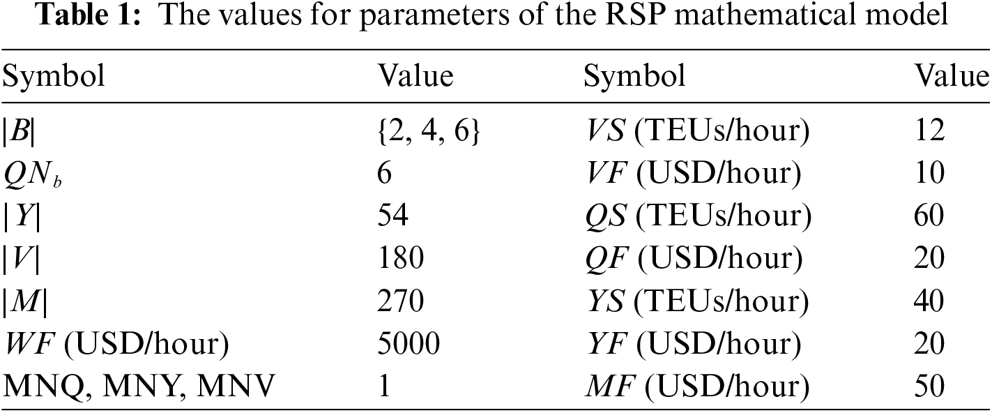
References in scheduling application literature [8,15] and actual data [1], the adopted values for parameters of the RSP mathematical model are presented in Table 1. There are three berthing availability cases: 2 berths, 4 berths, and 6 berths. There are 6 YCs can be deployed in each berth. Table 1 shows the maximum number of MCT resources (i.e., QNb, |Y|, |V|, and |M|) that can be scheduled at the same time. In addition, the working rate and cost of each equipment resource are also given.

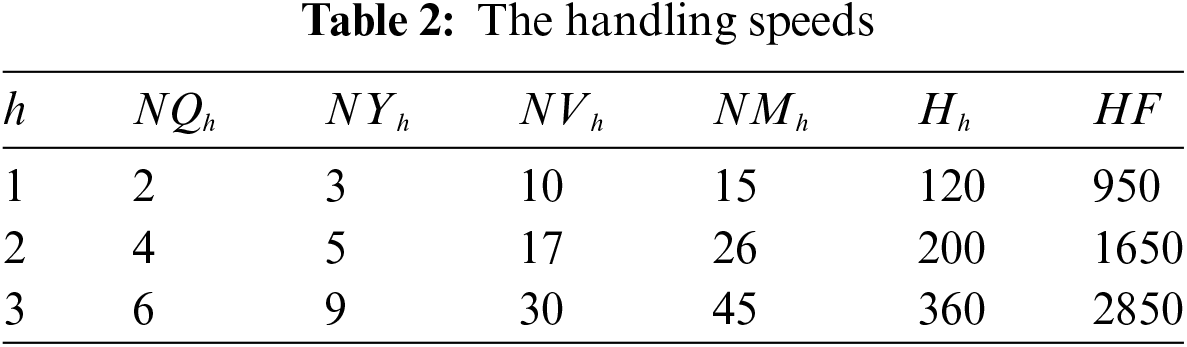
According to the above-known data, the handling speed is calculated by formula in Section 2.3. As shown in Table 2, there are 3 handling speeds meet the constraints (i.e., NH = 3). NQh needs to be an even number, so they are set 2, 4, and 6. The NYh are calculated by Eq. (2) and set to 3, 5, and 9. The NVh are computed by Eq. (3) and set to 10, 17, and 30. NMh are calculated by Eq. (4) and set to 15, 26, and 45. The Hh and HFh are calculated by Eqs. (5) and (6). The values of Hh are 120, 200, and 360. The corresponding values of HFh are 950, 1650, and 2850.

4.1.2 Parameters Configure for PACS

The parameter configurations are based on experimental verification of Section 4.3. The ACS-related parameters are introduced in this section. The population size (i.e., the number of ants) is set to |S| × |B|. The maximum generation is set to 1000 for every algorithm. The other parameters are set as follows: q0 = 0.6, β = 2, ρ = 0.9, ε = 0.1, ξ = 0.9.

4.1.3 Compared Algorithms for PACS

Herein, we select several state-of-the-art algorithms to compare with PACS, including SFLA (2023) [5], IVGGA (2022) [6], RCMGA (2022) [7], and AEA (2017) [8]. The compared algorithms cover a wide period from 2017 to 2023, providing a comprehensive evaluation on PACS. To make a fair comparison, all the compared algorithms share the same maximum fitness evaluations, while the other parameters in the compared algorithms are set the same as their original papers.

4.2 Test Cases

In test cases, the number of berths available is set to 2 berths, 4 berths, and 6 berths. The arrival time of ships is randomly generated by the exponential distribution with a mean of 2 h (i.e., ATs = E(2)). The number of containers to be loaded and unloaded by each ship is set to Cs = U(500, 2000) ( U-means the uniformly distributed). Two test case is used to compare the running results of six algorithms: FCFS, SFLA, IVGGA, RCMGA, AEA, ACS, and PACS. Note that “ACS” is PACS variant without pre-selection strategy. Moreover, the test results below are the average results of 50 dependent runs for each algorithm except FCFS.

4.2.1 Small Size Test Case

In small size test case (Case 1–Case 15), the number of ships changing from 16 to 20, and the number of berths changed from 2 to 6. The average fitness of the objective function of the RSP model is shown in Table 3.

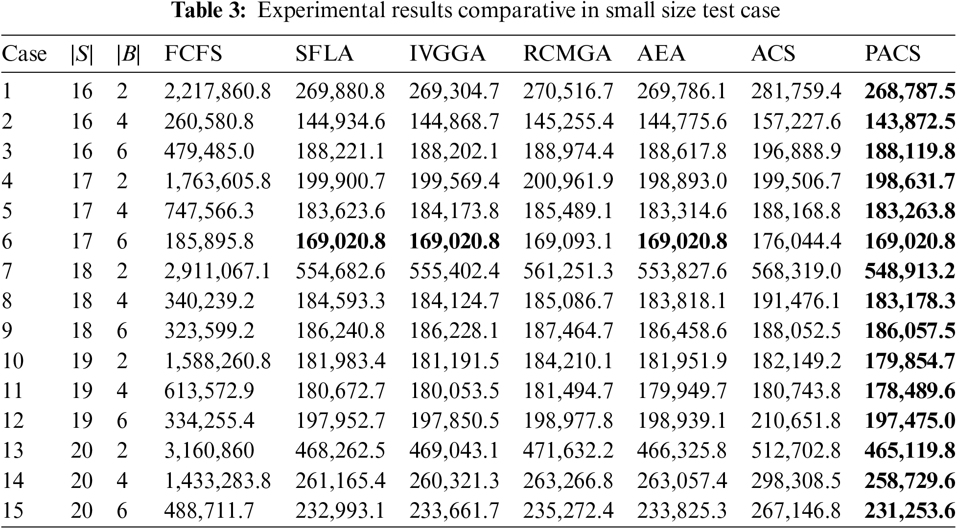
The experimental results in Table 3 show that the PACS algorithm can obtain the best results in the 15 test cases. It can be observed from Table 3 that FCFS gets the worst solutions in all the 15 cases, and the values of obtained solutions are quite large. This is because the wait cost is very expensive when the berthing sequence is not optimal. Moreover, the results of PACS are better than ACS, which shows the effectiveness of the pre-selection mechanism. From the results in Table 3, we can see that the PACS algorithm outperforms the SFLA, IVGGA, RCMGA, and AEA. IVGGA, RCMGA, and AEA are easy to produce infeasible solutions and the reinitialization will cause the slow convergence. From Table 3, we can see that SFLA, IVGGA, AEA and PACS achieve the same results in Case 6. That is because the solution of Case 6 is similar to the arrival order of the ships, while AEA adopts the first come first served mechanism in the initialization stage, and the optimal solution is easier to obtain. As shown in Table 3, SFLA and IVGGA seem suitable for solving large-scale problems, which can obtain the better results when there are more berths, such as in Case 6 and Case 9.

4.2.2 Large Size Test Case

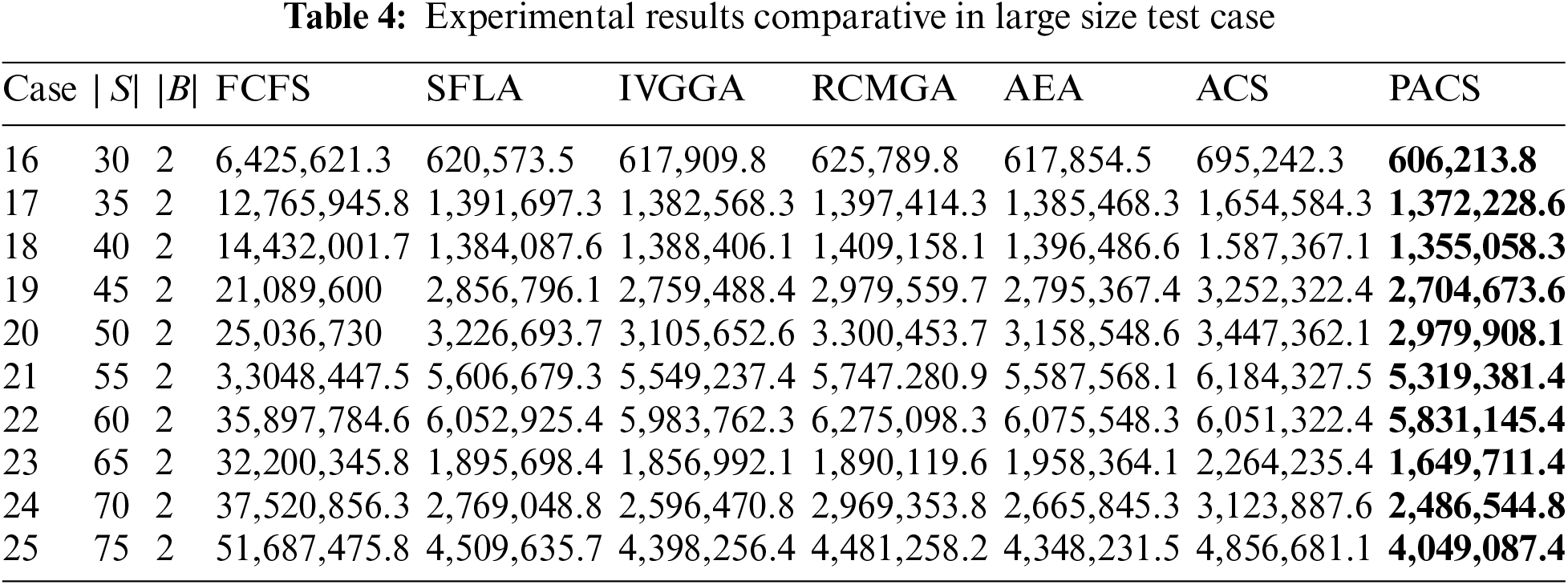
Table 4 lists the 10 test cases with 30 to 75 ships and 2 berths. The smaller the number of berths, the higher the average number of ships berthed at each berth, and the higher the density of ships, which is more matching with the large-scale environments. Therefore, the number of berths is set as 2. Different density test cases are used to test algorithms. In Cases 21 to 24, ships arrive more densely within similar times, resulting in more significant waiting costs. Cases 23 to 25 with more ships but arrival times scattered. As shown in Table 4, the PACS algorithm still can obtain the best results, and FCFS obtains the worst results. Besides, with the size and complexity of problem increase, the performance of SFLA, IVGGA, RCMGA, and AEA degrade rapidly. However, PACS still maintains the best global search ability to obtain the best results among all the compared algorithms, showing its promising ability in solving the large-scale RSP.

4.3 Analysis of PACS Parameters

The parameters in the PACS algorithm include q0, β, ρ, ε, and ξ. In order to study the influence of parameters on PACS algorithm performance, Case 13 and Case 16 are taken as an example for parameter analysis in this section. When we test one parameter, the other parameters remain the same as described above.

The investigation begins with the parameter q0. The parameter q0 is set as 0.1 to 0.9 with a step length of 0.1. Value 0 and 1 are not considered because the results are too bad to be drawn in Fig. 4a. The curves tend to decline with the value of q0 increases in Fig. 4a. However, a large q0 makes decreased the exploration ability of algorithm. Therefore, we set q0 = 0.6.

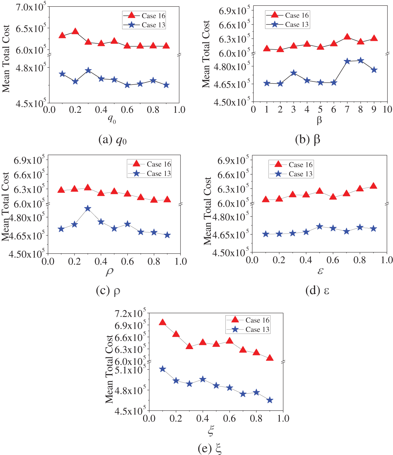
Figure 4: Influence of parameters. (a) q0, (b) β, (c) ρ, (d) ε, and (e) ξ

The next parameter tested is β. The parameter β is set from 1 to 9 with the interval 1. The value 0 is not considered because the solution is too bad to be plotted within Fig. 4b. For Case 13 and Case 16, when β = 2, PACS can get a better solution. So, we set β = 2.

Then parameters ρ and ε are investigated. The value of parameters ρ and ε are set as 0.1 to 0.9 with a step length of 0.1. When ρ and ε are 0 or 1, the results are too poor to not be plotted in Figs. 4c,d. When ρ = 0.9 and ε = 0.1, the PACS algorithm has better performance and gets better solutions. Therefore, we set ρ = 0.9 and ε = 0.1 in this paper.

Finally, parameter ξ in the pre-selection strategy is investigated. As shown in Fig. 4e, the solution quality is sensitive to ξ increase. The result for ξ = 0 is too poor and not shown in Fig. 4e. When parameter ξ = 1.0, the PACS algorithm lack of exploration and may converge to local optimality. Therefore, we set ξ = 0.9.

5  Conclusion

The efficiency of resource scheduling directly determines the operation performance in MCT. To solve the resources scheduling problem (RSP) in MCT effectively, this paper proposes an efficient ACS based on a pre-selection scheme (PACS), which contributes to both the problem model and algorithm design. In the problem model, different from other researches that only consider scheduling part of the resources in MCT, we designed a complete model of RSP by integrating multiple equipment-dependent parameters into one metric (i.e., handling speed). In this way, the RSP is modeled to find a scheduling scheme including berth allocation, berth time selection, and handling speed selection for every ship to minimize the total cost. In the algorithm design, the graphic structure is introduced to guarantee the feasibility of the solution. In addition, the pre-selection strategy is used to accelerate the convergence speed of the PACS algorithm. A large number of experimental results validate the effectiveness and efficiency of the proposed PACS algorithm, which can significantly outperform other state-of-the-art algorithms.

Although PACS achieves satisfying results, some parameters like pheromone decay parameter ρ and pre-selection parameter ξ are set according to the results of parameter sensitivity testing, which lacks the adaptive parameter mechanism. In the future, we wish to develop some adaptive parameter mechanisms in PACS to further improve its performance and also apply PACS to more complicated scheduling problems on MCT, even in multi-objective [35] and dynamic environments.

Acknowledgement: None.

Funding Statement: This research was supported in part by the National Key Research and Development Program of China under Grant 2022YFB3305303; in part by the National Natural Science Foundations of China (NSFC) under Grant 62106055, in part by the Guangdong Natural Science Foundation under Grant 2022A1515011825, and in part by the Guangzhou Science and Technology Planning Project under Grants 2023A04J0388 and 2023A03J0662.

Author Contributions: The authors confirm contribution to the paper as follows: Study conception and design: Rong Wang; data collection: Xinxin Xu, Nankun Mu; analysis and interpretation of results: Zijia Wang, Fei Ji; draft manuscript preparation: Rong Wang. All authors reviewed the results and approved the final version of the manuscript.

Availability of Data and Materials: The data are contained within the article.

Conflicts of Interest: The authors declare that they have no conflicts of interest to report regarding the present study.

References

1. UNCTAD, Review of Maritime Transport. 2023. Accessed: Sep. 27, 2023. [Online]. Available: https://unctad.org/topic/transport-and-trade-logistics/review-of-maritime-transport [Google Scholar]

2. “National cargo, container, and passenger throughput statistics-port network,” Accessed: Jan. 01, 2023. [Online]. Available: www.chinaports.com [Google Scholar]

3. G. D’Aniello, V. Loia, and F. Orciuoli, “An adaptive system based on situation awareness for goal-driven management in container terminals,” IEEE Intell. Transp. Syst. Mag., vol. 11, no. 4, pp. 126–136, Sep. 2019. doi: 10.1109/MITS.2019.2939137. [Google Scholar] [CrossRef]

4. V. D. Nguyen and K. H. Kim, “Heuristic algorithms for constructing transporter pools in container terminals,” IEEE Trans. Intell. Transp. Syst., vol. 14, no. 2, pp. 517–526, Jun. 2012. doi: 10.1109/TITS.2012.2222026. [Google Scholar] [CrossRef]

5. S. K. Jauhar, S. Pratap, S. Kamble, S. Gupta, and A. Belhadi, “A prescriptive analytics approach to solve the continuous berth allocation and yard assignment problem using integrated carbon emissions policies,” Ann. Oper. Res., pp. 1–32, Jul. 2023. [Google Scholar]

6. D. Yin, Y. F. Niu, J. Yang, and S. B. Yu, “Static and discrete berth allocation for large-scale marine-loading problem by using iterative variable grouping genetic algorithm,” J. Mar. Sci. Eng., vol. 10, no. 9, p. 1294, 2022. doi: 10.3390/jmse10091294. [Google Scholar] [CrossRef]

7. M. A. Hameed, W. M. Abed, R. K. Mohammed, and M. Yousaf, “Red monkey optimization and genetic algorithm to solving berth allocation problems,” Webology, vol. 19, no. 1, pp. 4888–4897, Jan. 2022. doi: 10.14704/WEB/V19I1/WEB19327. [Google Scholar] [CrossRef]

8. M. A. Dulebenets, “Application of evolutionary computation for berth scheduling at marine container terminals: Parameter tuning versus parameter control,” IEEE Trans. Intell. Transp. Syst., vol. 19, no. 1, pp. 25–37, Apr. 2017. doi: 10.1109/TITS.2017.2688132. [Google Scholar] [CrossRef]

9. N. Umang, M. Bierlaire, and I. Vacca, “Exact and heuristic methods to solve the berth allocation problem in bulk ports,” Transport. Res. E: Log., vol. 54, no. 3, pp. 14–31, Aug. 2013. doi: 10.1016/j.tre.2013.03.003. [Google Scholar] [CrossRef]

10. R. T. Cahyono, J. F. Engel, and B. Jayawardhana, “Discrete-event systems modeling and the model predictive allocation algorithm for integrated berth and quay crane allocation,” IEEE Trans. Intell. Transp. Syst., vol. 21, no. 3, pp. 1321–1331, Mar. 2019. doi: 10.1109/TITS.2019.2910283. [Google Scholar] [CrossRef]

11. E. Lalla-Ruiz, J. L. González-Velarde, B. Melián-Batista, and J. M. Moreno-Vega, “Biased random key genetic algorithm for the tactical berth allocation problem,” Appl. Soft. Comput., vol. 22, no. 2, pp. 60–76, Sep. 2014. doi: 10.1016/j.asoc.2014.04.035. [Google Scholar] [CrossRef]

12. Y. Li, F. Chu, F. Zheng, and M. Liu, “A bi-objective optimization for integrated berth allocation and quay crane assignment with preventive maintenance activities,” IEEE Trans. Intell. Transp. Syst., vol. 23, no. 4, pp. 2938–2955, Apr. 2022. doi: 10.1109/TITS.2020.3023701. [Google Scholar] [CrossRef]

13. Z. Cao, D. H. Lee, and Q. Meng, “Deployment strategies of double rail-mounted gantry crane systems for loading outbound containers in container terminals,” Int. J. Prod. Econ., vol. 115, no. 1, pp. 221–228, Sep. 2008. doi: 10.1016/j.ijpe.2008.05.014. [Google Scholar] [CrossRef]

14. R. T. Cahyono, S. P. Kenaka, and B. Jayawardhana, “Simultaneous allocation and scheduling of quay cranes, yard cranes, and trucks in dynamical integrated container terminal operations,” IEEE Trans. Intell. Transp. Syst., vol. 23, no. 7, pp. 8564–8578, Jul. 2022. doi: 10.1109/TITS.2021.3083598. [Google Scholar] [CrossRef]

15. H. Li, J. Peng, X. Wang, and J. Wan, “Integrated resource assignment and scheduling optimization with limited critical equipment constraints at an automated container terminal,” IEEE Trans. Intell. Transp. Syst., vol. 22, no. 12, pp. 7607–7618, Dec. 2021. doi: 10.1109/TITS.2020.3005854. [Google Scholar] [CrossRef]

16. S. Tanaka and K. Takii, “A faster branch-and-bound algorithm for the block relocation problem,” IEEE Trans. Autom. Sci. Eng., vol. 13, no. 1, pp. 181–190, Jun. 2015. doi: 10.1109/TASE.2015.2434417. [Google Scholar] [CrossRef]

17. X. Xiang, L. H. Lee, and E. P. Chew, “An adaptive dynamic scheduling policy for the integrated optimization problem in automated transshipment hubs,” IEEE Trans. Autom. Sci. Eng., Early Access, Apr. 21, 2023. [Google Scholar]

18. G. Maione, A. M. Mangini, and M. Ottomanelli, “A generalized stochastic Petri net approach for modeling activities of human operators in intermodal container terminals,” IEEE Trans. Autom. Sci. Eng., vol. 13, no. 4, pp. 1504–1516, Oct. 2016. doi: 10.1109/TASE.2016.2553439. [Google Scholar] [CrossRef]

19. X. F. Ye, Y. L. Wang, X. C. Yan, W. Tao, and J. Chen, “Optimization model of autonomous vehicle parking facilities, developed with the nondominated sorting genetic algorithm with an elite strategy 2 and by comparing different moving strategies,” IEEE Intell. Transp. Syst. Mag., vol. 15, no. 3, pp. 82–100, May 2023. doi: 10.1109/MITS.2022.3220778. [Google Scholar] [CrossRef]

20. C. Liang, J. Guo, and Y. Yang, “Multi-objective hybrid genetic algorithm for quay crane dynamic assignment in berth allocation planning,” J. Intell. Manuf., vol. 22, no. 3, pp. 471–479, 2011. doi: 10.1007/s10845-009-0304-8. [Google Scholar] [CrossRef]

21. Y. Jiang, Z. H. Zhan, K. C. Tan, and J. Zhang, “Knowledge learning for evolutionary computation,” IEEE Trans. Evol. Comput., 2023. doi: 10.1109/TEVC.2023.3278132. [Google Scholar] [CrossRef]

22. Z. H. Zhan, J. Y. Li, S. Kwong, and J. Zhang, “Learning-aid evolution for optimization,” IEEE Trans. Evol. Comput., vol. 27, no. 6, pp. 1794–1808, Dec. 2023. doi: 10.1109/TEVC.2022.3232776. [Google Scholar] [CrossRef]

23. C. Liang, Y. Huang, and Y. Yang, “A quay crane dynamic scheduling problem by hybrid evolutionary algorithm for berth allocation planning,” Comput. Ind. Eng., vol. 56, no. 3, pp. 1021–1028, Apr. 2009. doi: 10.1016/j.cie.2008.09.024. [Google Scholar] [CrossRef]

24. S. H. Wu, Z. H. Zhan, and J. Zhang, “SAFE: Scale-adaptive fitness evaluation method for expensive optimization problems,” IEEE Trans. Evol. Comput., vol. 25, no. 3, pp. 478–491, Jun. 2021. doi: 10.1109/TEVC.2021.3051608. [Google Scholar] [CrossRef]

25. J. He, Y. Huang, and W. Yan, “Yard crane scheduling in a container terminal for the trade-off between efficiency and energy consumption,” Adv Eng. Informat., vol. 29, no. 1, pp. 59–75, Jan. 2015. doi: 10.1016/j.aei.2014.09.003. [Google Scholar] [CrossRef]

26. M. A. Dulebenets, R. Moses, E. E. Ozguven, and A. Vanli, “Minimizing carbon dioxide emissions due to container handling at marine container terminals via hybrid evolutionary algorithms,” IEEE Access, vol. 5, pp. 8131–8147, Apr. 2017. doi: 10.1109/ACCESS.2017.2693030. [Google Scholar] [CrossRef]

27. A. Colorni, M. Dorigo, and V. Maniezzo, “Distributed optimization by ant colonies,” presented at the Proc. First Eur. Conf. Artif. Life, Paris, France, Dec. 11, 1992. [Google Scholar]

28. M. Dorigo and L. M. G. ambardella, “Ant colony system: A cooperative learning approach to the traveling salesman problem,” IEEE Trans. Evol. Comput., vol. 1, no. 1, pp. 53–66, Apr. 1997. doi: 10.1109/4235.585892. [Google Scholar] [CrossRef]

29. X. Zhang, Z. H. Zhan, W. Fang, P. J. Qian, and J. Zhang, “Multipopulation ant colony system with knowledge-based local searches for multiobjective supply chain configuration,” IEEE Trans. Evol. Comput., vol. 26, no. 3, pp. 512–526, Jun. 2022. doi: 10.1109/TEVC.2021.3097339. [Google Scholar] [CrossRef]

30. D. Wu, Z. Zhu, D. Hu, and R. F. Mansour, “Optimizing fresh logistics distribution route based on improved ant colony algorithm,” Comput. Mater. Contin., vol. 73, no. 1, pp. 2079–2095, 2022. doi: 10.32604/cmc.2022.027794. [Google Scholar] [CrossRef]

31. X. F. Liu, Z. H. Zhan, J. D. Deng, Y. Li, T. L. Gu and J. Zhang, “An energy efficient ant colony system for virtual machine placement in cloud computing,” IEEE Trans. Evol. Comput., vol. 22, no. 1, pp. 113–128, Feb. 2018. doi: 10.1109/TEVC.2016.2623803. [Google Scholar] [CrossRef]

32. A. Sharif et al., “Traffic management in internet of vehicles using improved ant colony optimization,” Comput. Mater. Contin., vol. 75, no. 3, pp. 5379–5393, 2023. doi: 10.32604/cmc.2023.034413. [Google Scholar] [CrossRef]

33. G. Chen, D. Cheng, W. Chen, X. Yang, and T. Guo, “Path planning for AUVs based on improved APF-AC algorithm,” Comput. Mater. Contin., vol. 78, no. 3, pp. 3721–3741, 2024. doi: 10.32604/cmc.2024.047325. [Google Scholar] [CrossRef]

34. R. Wang et al., “An adaptive ant colony system based on variable range receding horizon control for berth allocation problem,” IEEE Trans. Intell. Transp. Syst., vol. 23, no. 11, pp. 21675–21686, Nov. 2022. doi: 10.1109/TITS.2022.3172719. [Google Scholar] [CrossRef]

35. J. Y. Li, Z. H. Zhan, Y. Li, and J. Zhang, “Multiple tasks for multiple objectives: A new multiobjective optimization method via multitask optimization,” IEEE Trans. Evol. Comput., Jul. 2023. doi: 10.1109/TEVC.2023.3294307. [Google Scholar] [CrossRef]