Physics-Constrained Robustness Enhancement for Tree Ensembles Applied in Smart Grid

Nomenclature/Abbreviation

1  Introduction

Smart grids integrate advanced information technology deeply with power systems, achieving intelligent operation and management of the grid. A large number of measurement and control devices are incorporated into smart grids to meet the needs of complex tasks such as environmental monitoring and real-time control [1]. As the number of smart grid terminals increases, communication between devices significantly grows [2], generating massive amounts of heterogeneous, multidimensional data. Smart grids are gradually adopting machine learning models to efficiently analyze and process data in areas such as power monitoring, fault diagnosis [3], outage detection [4], and demand response [5]. This adoption enables intelligent analytical decisions and improves the operational efficiency and management level of the grid.

However, numerous studies have shown that machine learning is susceptible to adversarial attacks [6,7]. Adversarial attacks on machine learning aim to deceive or disrupt the operation of machine learning systems by adding small, malicious perturbations to normal data. For example, in the field of image processing, by slightly modifying the pixels of an image, a machine learning model might mistakenly identify an ordinary object as a completely different one. This type of attack can lead to severe consequences in critical applications such as autonomous driving and facial recognition systems.

Due to the characteristics of smart grids, the attack surface for ML applications in smart grids is broader than in applications involving images or audio. As the number of smart grid devices connected to the internet increases, the number of entry points for attackers also rises [8]. Additionally, as more Operational Technology networks connect with Information Technology networks, many traditional devices lacking high-security standards are easily manipulated by attackers [9]. This allows attackers to add perturbations to the raw data transmitted or received by these devices. In the context of smart grids, raw data from devices such as Precision Measurement Units (PMU) and Remote Terminal Units (RTU) are susceptible to tampering during transmission. For example, Rajkumar et al. [10,11] have identified vulnerabilities in the IEC 61850 standard, which is widely used for substation automation and protection. These vulnerabilities can be exploited by attackers to launch network attacks, such as data injection attacks and adversarial attacks. Globally, there have been several cyber-attack incidents on smart grids that have resulted in significant economic losses [12–14]. Thus, in smart grids, ML has become a new security vulnerability point in cyber-attacks [15,16].

In ML, Neural Networks (NN) are known for their high accuracy, while tree ensemble models are favored in smart grid applications for their better interpretability and simpler structure [17]. In the industry, tree ensembles have been validated in several actual energy management systems in Europe and Canada [18,19]. For example, the iTesla project developed a security assessment toolbox based on tree ensembles to support stable decision-making in the pan-European transmission system [19]. Stability assessments of power systems based on tree ensembles have been applied and validated in the energy system of New Orleans [20]. However, smart grid applications based on tree ensembles also face security threats caused by system vulnerabilities, where attackers can launch adversarial attacks through these vulnerabilities. Robustness is a key metric for measuring ML model’s performance under adversarial attacks. It evaluates the model’s ability to resist attacks and maintain efficient operation. Therefore, enhancing the robustness of tree ensemble models is crucial to ensure the safety and efficiency of smart grid applications in adversarial environments.

Madry et al. [21] described enhancing robustness as a min-max problem, and this principle can be applied to tree ensemble models through various strategies. For example, Kantchelian et al. [22] adopted an adversarial training approach similar to that used for NN (Szegedy et al. [23]), where the training set is enriched with adversarial examples. Moreover, several studies have proposed optimizing the splitting process of tree ensembles to improve robustness. Chen et al. [24], Vos et al. [25], and Chen et al. [26] developed methods to refine the decision tree node splitting process, focusing on setting split thresholds away from data-dense areas to prevent adversarial examples from easily crossing these thresholds with minimal perturbation. These traditional robustness enhancement methods, while effective in many domains, face unique challenges when applied to smart grids. Unlike other applications, smart grid systems must address real-world problems involving sensor data that have specific physical meanings and are constrained by physical laws. This necessity requires robustness enhancement strategies for tree ensembles in smart grids to consider these physical constraints. This consideration ensures the realism of adversarial attacks and the genuine robustness of the model.

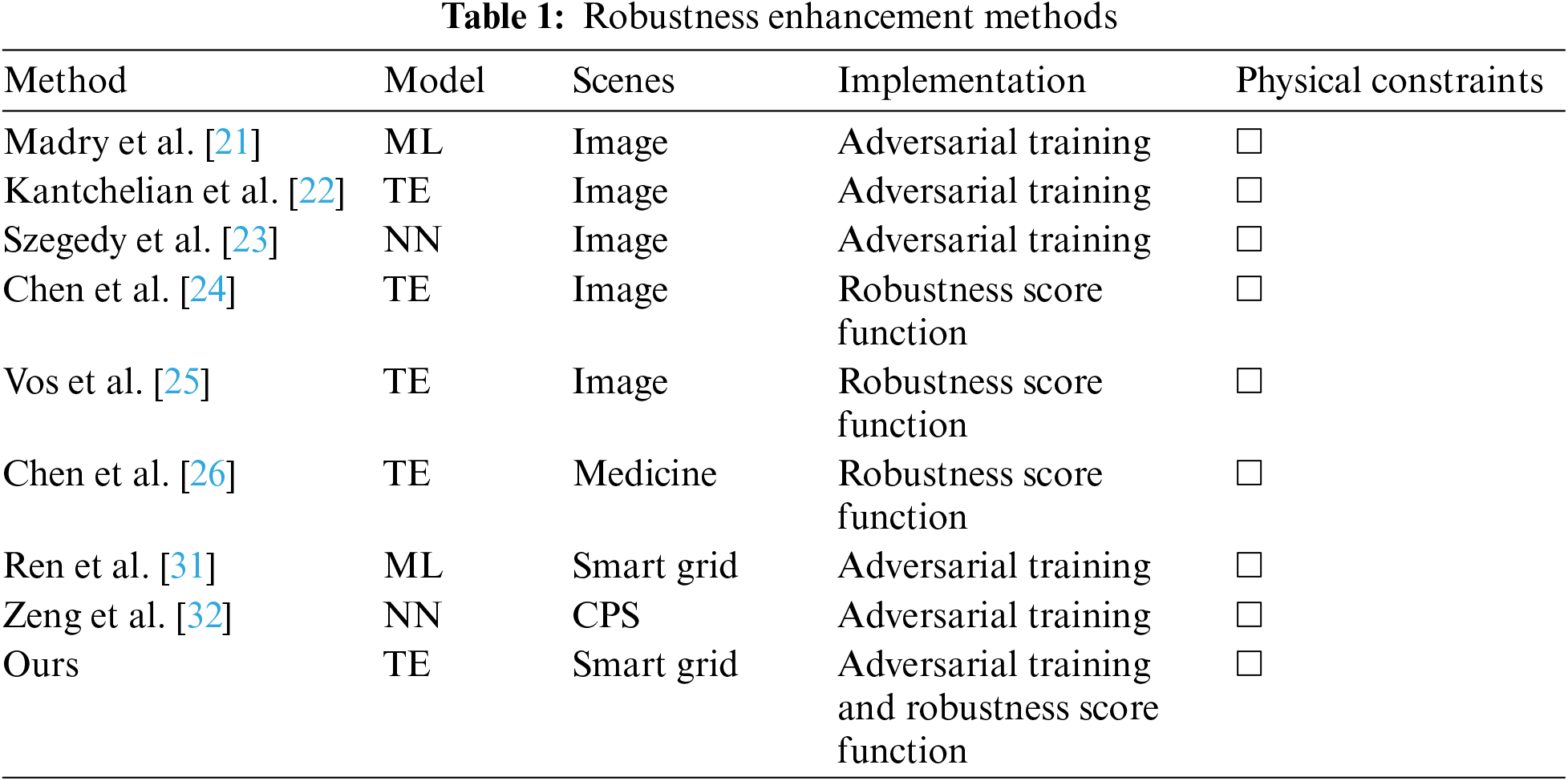
In the context of smart grids, adversarial training is the most well-known method for enhancing the robustness of machine learning-based applications [27–30]. Ren et al. [31] considered black-box adversarial training to train an ensemble agent model based on machine learning applications to mitigate adversarial examples. Zeng et al. [32] proposed a periodic adversarial training method to learn how to handle adversarial attacks. However, as shown in Table 1, these robustness enhancement methods for smart grid applications are all based on NN. They do not consider the discrete, non-differentiable nature of tree ensemble, nor do they account for the need for adversarial attacks to comply with physical constraints.

Thus, while the existing literature provides a foundation, it becomes essential to explore how these ideas can be adapted into more practical strategies tailored to smart grid environments. By integrating physical constraints into adversarial training and decision tree splitting processes, we can develop robustness enhancement methods specifically designed for smart grids. This approach ensures that the adversarial examples and the corresponding model training processes comply with the physical realities of smart grid operations. This compliance ultimately leads to more effective and reliable robustness enhancement strategies.

Therefore, this paper aims to enhance the robustness of tree ensemble applications in smart grids effectively. However, achieving this goal presents challenges. First, the complex relationship between the physical constraint space and the tree ensemble feature space makes it difficult to confine robustness enhancements within the physical constraint space. Second, the feature thresholds of tree ensemble node splits cannot guarantee compliance with physical constraints. These challenges are addressed using the following methods: adversarial examples that comply with physical constraints are used for adversarial training, ensuring that the learning of robustness enhancement aligns with physical constraints. Physical constraints are transformed into constraints on node splitting thresholds, allowing the ensemble tree to classify data in the physical constraint space. In summary, the contributions are as follows:

•   A dataset of adversarial examples that comply with physical constraints is generated using a minimal perturbation adversarial attack method for tree ensembles that comply with physical constraints. This dataset is used for adversarial training, enhancing the robustness of tree ensembles under physical constraints.

•   Physical constraints are incorporated into the tree ensemble node splitting process that focuses on robustness, thereby enhancing the robustness of tree ensembles within physical constraints.

•   Real-world grid data is used for experiments to validate the feasibility and effectiveness of the proposed methods.

2  Robustness Enhancement Method

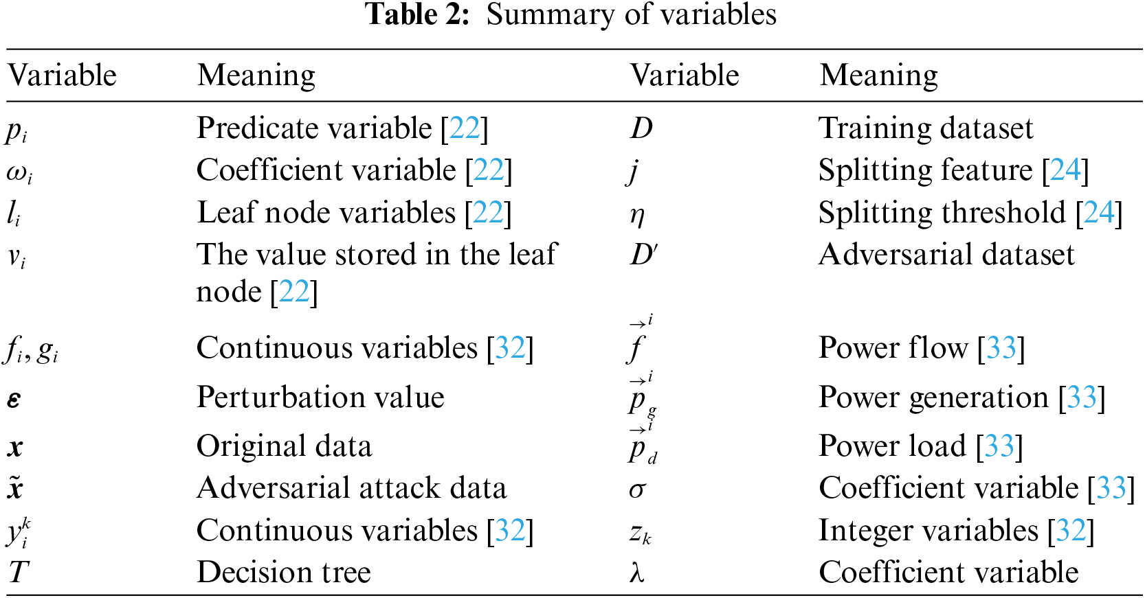
A Summary of variables is shown in Table 2.

2.1 Adversarial Training

Adversarial training was initially used in NN. Its core idea is to continuously generate adversarial examples during the training process and incorporate these adversarial examples into the training data. This approach ensures that the model minimizes the loss function of adversarial examples while optimizing parameters. This training strategy has been proven to significantly enhance the robustness of NN against adversarial attacks.

The idea of adversarial training can also be applied to tree ensemble models. Specifically, when constructing each decision tree, it is necessary not only to minimize the loss function of the original data but also to minimize the loss function of adversarial examples. This means that when selecting the optimal splitting feature and threshold for each node, it is necessary to consider two objectives. First, minimize the loss function of the original training data to ensure that most training data are correctly classified. Second, minimizing the loss function of adversarial examples to ensure that the model’s predictions do not change even in the presence of adversarial perturbations. Formally, the loss function of a decision tree can be defined as

Loss(T)=(1−λ)Lossnat(T)+λLossadv(T)(1)

where, T is the current decision tree, Lossnat(T) is the loss on the original undisturbed data, and Lossadv(T) is the loss on adversarial examples. λ∈[0,1] controls the trade-off between natural and adversarial examples. For each node split, the optimal feature and threshold are chosen to minimize both loss functions simultaneously.

During the training of Random Forests or Gradient Boosting decision trees (GBDT), for each new decision tree generated, a batch of adversarial examples can be created based on the existing tree ensemble model. The loss of the new decision tree on these adversarial examples is then minimized. Specifically, for Random Forests, the traditional splitting rule of Gini impurity or information gain can be modified. The splitting rule of the traditional Gini coefficient is as follows:

Gini(D,j)=1−∑i=1Np(i|D)2(2)

where, D represents the data at the current node, j is the splitting feature, and p(i|D) represents the proportion of data belonging to class i. N is the total number of data points. It can be modified to

Gini′(D,j)=(1−λ)Gini(Dnat,j)+λGini(Dadv,j)(3)

where Dnat represents the original training data at the node, and Dadv represents the adversarial example data. The weight λ controls the trade-off between these two parts. In searching for the optimal splitting feature, the modified criterion is minimized Gini′(D,j).

For GDBT, the traditional regression tree node splitting rules can be modified. Take minimizing the squared loss as an example,

Loss(T)=∑(yi−f(xi))2(4)

where, yi represents the actual labels of the data point i, and f(xi) the model’s predicted output on the data point i. It can be modified to

Loss′(T)=(1−λ)∑(yi−f(xi))2+λ∑(zi−f(x~i))2(5)

where, x~i represents the adversarial examples, and zi represents the expected output for the adversarial examples (for instance, zi=yi for unattacked data; zi=−yi for adversarial examples). Similarly, the modified loss is minimized during node splitting.

With the above modifications, we can integrate robustness considerations into every node split during the construction of the decision tree. The trees generated are not only expected to have good classification performance on the original data, but are also designed to resist perturbations to the greatest extent. This ensures that their prediction output remains unchanged in the face of adversarial attacks. For the entire Random Forest or GBDT, as it is composed of many such robust decision trees, it naturally achieves stronger resistance to adversarial attack.

It should be noted that adversarial training often increases the computational cost. The reason is that training needs to be performed not only on the original data but also on the generated adversarial examples. Therefore, for training Random Forests or GBDT, there are generally the following strategies.

Full Adversarial Training: Each new decision tree generated in each round is trained using adversarial training. This process involves generating adversarial examples based on the current tree ensemble model and minimizing the loss of these examples for the new tree. This strategy offers the greatest increase in robustness but also incurs significant computational costs.

Periodic Adversarial Training: Adversarial training is conducted at fixed intervals (e.g., every 10 rounds). This method reduces computational costs but also results in a smaller increase in robustness.

Partial Adversarial Training: During the entire training process, only a portion of the decision trees (e.g., the last 20% of trees) undergo adversarial training. This approach allows for a reasonable increase in robustness with acceptable computational costs.

2.2 A General Framework for Training Robust Decision Trees

Adversarial training for tree ensemble models is mainly achieved through post-hoc data augmentation, which faces several issues. The limitations of this approach include the inability to update the initial trees, the rapid obsolescence of the generated adversarial examples, high computational overhead, and limited gains in robustness. The underlying issue stems from the absence of robustness optimization during the construction of each tree, which hinders the model’s ability to fundamentally improve its robustness from the ground up. Therefore, robustness considerations should be introduced at the most fundamental unit of decision tree construction to fundamentally overcome the limitations of traditional adversarial training for tree ensembles.

Conventional decision tree training processes greedily select the optimal split features and thresholds, which can be vulnerable to adversarial attacks. To train decision tree models with robustness against adversarial perturbations, Chen et al. [24] proposed a novel training framework. This framework incorporates the consideration of worst-case adversarial perturbations into the selection of optimal splits, thereby yielding robust decision trees.

Traditional decision tree construction typically uses a greedy approach, selecting the best splitting feature and threshold at each node. This selection is based on achieving optimal performance on a score function, such as information gain or Gini coefficient, in the resulting child nodes.

(j∗,η∗)=argmaxj,ηS(j,η,D)(6)

where, S(⋅) represents information gain or the Gini coefficient. j* is the optimal splitting feature, and η∗ is the optimal splitting threshold. D represents the training data. However, this standard approach only considers the distribution of the data itself and does not account for potential adversarial perturbations. When faced with adversarial attacks, attackers can subtly modify the features of the data to cross splitting boundaries, leading to classification errors and demonstrating the lack of robustness in decision trees.

To address this issue, a robustness score function needs to be introduced into the decision tree construction process. This function differs from traditional score functions in that it considers potential adversarial perturbations on each feature, aiming to minimize the loss in the worst-case scenario (i.e., the most aggressive perturbations). Specifically, during each node splitting, the original score function is no longer used; instead, the following robustness score is optimized:

(j∗,η∗)=argmaxj,ηRS(j,η,D)(7)

where RS(⋅) represents the robustness score function. j* is the optimal splitting feature, and η∗ is the optimal splitting threshold. D represents the training data. RS(⋅) is defined as

RS(j,η,D)=minD′={(x~i,yi)}S(j,η,D′)(8)

s.t.x~i∈Bε(xi)∞(xi),∀x~i∈D′(9)

Bε(xi)∞:=[xi(1)−ε,xi(1)+ε]×[xi(2)−ε,xi(2)+ε]×⋯×[xi(d)−ε,xi(d)+ε](10)

where, S(j,η,D′) represents the original score function used for splitting based on feature j and threshold η on the dataset D′ after adversarial perturbation. Bε(xi)∞denotes the ℓ∞ ball ε-neighborhood around xi, which includes all possible adversarial examples that do not exceed perturbations of ε on each feature. This robustness score function considers the score under the worst-case scenario. Maximizing it means finding a split such that the decline in classification performance is minimized across all possible adversarial perturbations. Intuitively, this encourages the decision tree to learn a splitting method that is robust against adversarial perturbations.

Since the minimization problem is difficult to solve directly, Chen et al. [24] proposed two approximate algorithms: For classification trees based on information gain, they proved that the optimal adversarial strategy is to move data points within the ε-neighborhood of the splitting threshold as uniformly as possible into the two child nodes. They also provided a linear-time greedy algorithm to approximate the robust split. For GBDT, optimizing all trees simultaneously rather than a single tree makes directly solving the robustness score function computationally expensive. Therefore, they considered four representative adversarial perturbation scenarios to approximate the worst-case situation, and the minimum value is taken as the approximate robustness score.

3  Robustness Enhancement Method with Physical Constraints

In smart grid scenarios, the methods from Section 2.2 and adversarial training techniques for enhancing model robustness both face certain issues. Firstly, they typically assume that an adversary can perturb data points within a predefined range. However, under physical constraints, perturbations may be subject to more complex restrictions, such as correlations between features and nonlinear constraints, which these methods do not address. Secondly, different features often carry different physical meanings, units, and numerical ranges. Applying a uniform perturbation magnitude, as suggested in Section 2.2, may result in perturbations that are either unreasonable or insufficient for some features. Then, setting an appropriate perturbation range for each feature increases the difficulty of optimization. Moreover, although the adversarial examples used in adversarial training are mathematically feasible, they might be unachievable or non-existent in the physical world. As shown in Fig. 1, we need methods that can enhance robustness within the boundaries of physical constraints.

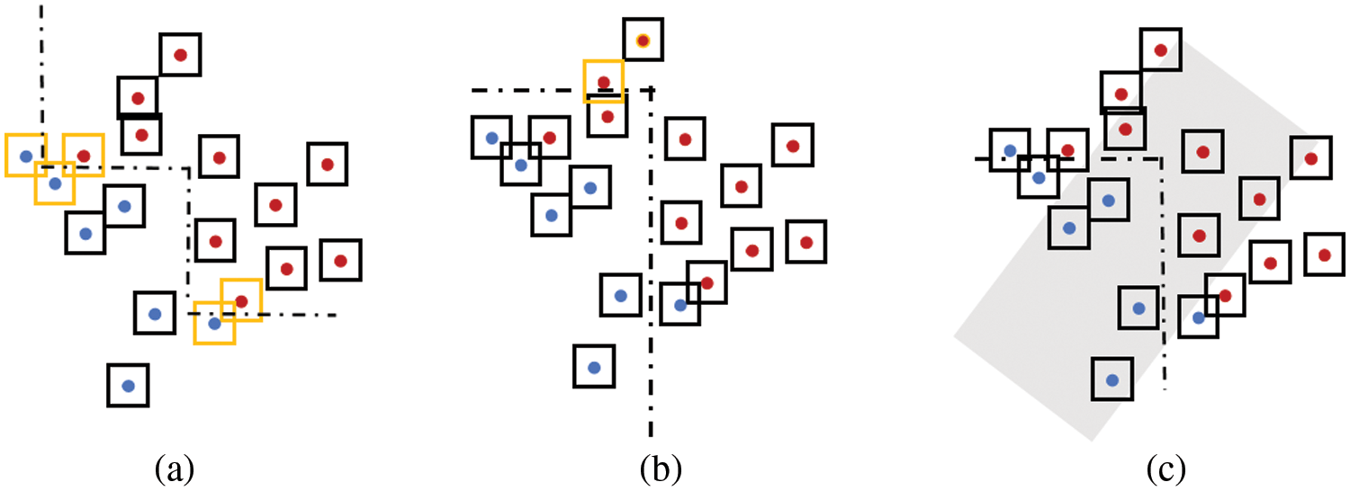
Figure 1: Schematic diagram of the classification of tree ensemble under different training methods. The red and blue data points in the figure represent different categories. The box outside the point indicates the infinite norm range of the r radius. When the box is black, the point is robust within the range. When the box is orange, the point is not robust within the range. The gray area is the restraint interval. (a) Classification of tree ensemble without physical constraints. (b) Classification after robustness enhancement of tree ensemble without physical constraints. (c) Classification with enhanced robustness of the tree ensemble under physical constraints

3.1 Adversarial Training with Physical Constraint

Adversarial training requires the assistance of corresponding adversarial examples. When there are no physical constraints, Kantchelian et al. [22] proposed a general method for generating adversarial attacks for tree ensembles, formulated as the following optimization problem:

minpi,li∑i∈𝒫ωipi+C

s.t.p1i≤p2i≤⋯≤pMi

l1+l2+⋯+lM′=1

1−(l1f+l2f+⋯+ljf)=ps=l1t+l2t+⋯+lit(11)

1−(l1r,f+l2r,f+⋯+ljr,f)≥pr≥l1r,f+l2r,f+⋯+lir,f

f(x~)=∑i∈ℓvili≥0

In the optimization problem (11), the modeling process of generating adversarial examples by the ensemble tree model does not take into account equality constraints and inequality constraints. Therefore, it is necessary to describe physical constraints using predicate variables and leaf variables, incorporating them into the modeling process. In this paper, we consider linear constraints to simplify the discussion. The equation constraints can be expressed as follows:

Aε=u(12)

where, A is a coefficient matrix, and u is a constant vector. The inequality constraints can be expressed as follows:

Bε≤v(13)

where, B is a coefficient matrix and v is a constant vector. According to [33], the method for solving for adversarial examples under physical constraints is formulated as the following optimization problem:

minpi,li,fi,gi,zik,ε∑ifi+gi

s.t.fi≥0,gi≥0

x~i=fi−gi+xi

akzk≤yik≤ak+1zk

zk=pki−pk+1i

x~=1TY

x~=x+ε(14)

Bε≤v

Aε=u

p1i≤p2i≤⋯≤pMi

l1+l2+⋯+lM′=1

1−(l1f+l2f+⋯+ljf)=ps=l1t+l2t+⋯+lit

1−(l1r,f+l2r,f+⋯+ljr,f)≥pr≥l1r,f+l2r,f+⋯+lir,f

f(x~)=∑i∈ℓvili≥0

This optimization problem involves finding adversarial examples with the minimum perturbation under the ℓ1 norm, adhering to constraints (12) and (13). This minimal perturbation can be used to assess the robustness of tree ensembles that adhere to physical constraints.

3.2 Robust Decision Tree Training with Physical Constraints

To introduce physical constraints into robust decision trees, we can enhance the methods discussed in Section 2.2. Suppose we have a set of linear physical constraints, including equation constraints (12) and inequality constraints (13). For each feature dimension j, we can determine the upper and lower bounds of feature values, ηjmin and ηjmax, by solving the solution space of these constraints.

First, we express the linear equation constraint Ax=u using the general solution of a nonhomogeneous linear,

x=xp+xn(15)

where, xp is a particular solution of Ax=u, and xn is the general solution of Ax=0. We can use Gaussian elimination to find xp, and then derive the expression for xn by solving Ax=0.

xn=c1v1+c2v2+…+ckvk(16)

where, v1,v2,…,vk are the fundamental systems of solutions of Ax=0 and c1,c2,…,ck are arbitrary constants. Substituting (15) into the linear inequality constraint Bx≤v, we can obtain:

ηmin≤x≤ηmax(17)

After determining the range [ηjmin,ηjmax] for each feature xj, the threshold ηj for each feature xj must also satisfy the inequality (17). We incorporate (17) into the existing robustness score function,

RS(j,η,D)=minI′={(x~i,yi)}S(j,η,D′)

s.t.x~i∈Bε(xi)∞(xi),∀x~i∈D′(18)

ηmin≤η≤ηmax

By introducing upper and lower bounds on feature values, we ensure that perturbed data points comply with physical constraints. To solve this optimization problem, we only need to include checks for η in the solution method described in [24].

Combining physically constrained adversarial training with improved robust decision tree methods can further enhance the model’s robustness. This combination leverages the adaptability of adversarial training and the explicit optimization of robustness during the training process of robust decision trees. For example, in GBDT, we can consider the following combination approach:

Step 1: Solve the optimization problem (18) such that the optimal split for each decision tree is selected during construction.

Step 2: After each round of Boosting iterations, use optimization problem (14) to generate adversarial examples that comply with physical constraints.

Step 3: Incorporate the generated adversarial examples into the training set for use in subsequent Boosting iterations.

Repeat steps 1–3 until the predetermined number of Boosting rounds is reached or the early stopping criteria are met. During this process, the model continuously balances robustness and accuracy and adapts to the changing distribution of adversarial examples.

By integrating these steps, we have developed an algorithm that combines physically constrained adversarial training with robust decision tree methods. This combination is expected to enhance model robustness while ensuring that the generated adversarial examples and the learned decision boundaries comply with physical constraints. As a result, this improves the model’s applicability in real-world physical environments.

4  Experiment

4.1 Physical Constraints of Smart Grids

The security-constrained Direct Current optimal power flow (SC-DCOPF) problem is an optimization problem that considers the power system N−1 security constraints [34]. It is formulated based on a traditional DCOPF model by adding security constraints for N−1 fault conditions. The basic idea is to ensure that the system remains secure and stable in the event of any N−1 category failures. In this scenario, the perturbation εi can be defined as

εi=[Δf→i;Δp→gi;Δp→di](19)

The changes in f→, p→g, and p→d are thus represented by εi, which forms the basis for the bad data detection (BDD). BDD is a method for detecting erroneous data in power grids. The optimization adjusts the power generation to reach the optimal state while considering the security constraints. In this context, the constraints are given as follows:

∑Δp→di=0(20)

−σΔp→di≤Δp→di≤σΔp→di,σ∈[0,1](21)

Δf→i=−SCH−1Δp→di(22)

In the above, σΔp→di is the standard deviation of the adjustments in demand, which should be kept within limits. The last equation relates to the changes in the power flow Δf→i, which are inversely proportional to the changes in demand.

4.2 Datasets and Evaluation Metrics

The following is an evaluation of the performance improvement of the robustness enhancement strategy. This improvement is quantified by comparing the operational performance of the system before and after the application of the robustness enhancement strategy.

The robustness enhancement strategy performance improvement D* is calculated as

D∗=1N∑i=1ND(xi,xi+εi∗)D(xi,0)(23)

Here, D(xi,xi+εi∗) represents the operational performance of the system under the robustness enhancement strategy, and D(xi,0) represents the operational performance under normal conditions. N is the total number of data points. xi is a data point in training dataset. The metric indicates the relative performance enhancement. We use (14) to calculate the minimum perturbation εi∗.

The number of defined robust data points is also used to quantify the robustness of the ML model. In some cases, given a specific robust data point, there may not exist a feasible solution to the robustness evaluation problem, which highlights the importance of this metric. For this data point, the attacker cannot interfere with it and change its predictions. The ratio of robust data points is used as a physical constraint robustness evaluation metric,

RP=ThenumberofrobustdatapointsThenumberofalldatapoints(24)

The dataset used in this chapter was generated based on SC-DCOPF. We consider seven contingencies by cutting off transmission lines {2, 4} (T1), {3, 4} (T2), {6, 12} (T3), {6, 13} (T4). The test dataset used takes into account that the data collected in the power system scenario is susceptible to noise interference, such as sudden fluctuations in power load and sensor failures. Therefore, it requires appropriate preprocessing and cleaning to improve the accuracy and reliability of subsequent analysis. Our data is derived from 12,000 load configurations sampled from real load data traces in New York State injected into an IEEE 14-node power system in a public dataset [35]. Use the default parameters of the IEEE 14-node power system provided by MATPOWER. If the stability condition is violated, the corresponding data is marked as “0”; otherwise, the data is marked as “1”. In total, we use 12,000 labeled data points to train and test the ensemble tree-based Static Security Assessment (SSA) model and verify the robustness of XGBoost under different parameter settings. Next, C1 represents the adversarial attack constraint. C2 represents the inequality constraint (12). C3 represents the equality constraint (13).

4.3 Experimental Results

The experimental platform we used is configured with an i7-10875H CPU, an RTX2060 GPU, 16 GB of memory, and a 512 GB SSD. The operating system is Windows 10, and the experimental environment runs on Python 3.8. We used Gurobi 10.0.2 as the solver. The two main ensemble tree models we utilized are XGBoost and Random Forest. The XGBoost parameters were set to tree number = 50, learning_rate = 0.9, subsample = 0.8, and max_depth = 6. The Random Forest parameters were tree number = 100, learning_rate = 0.8, subsample = 0.8, and max_depth = 6.

The original dataset used in this section is generated based on SC-DCOPF. The dataset of unconstrained adversarial examples is generated by solving optimization problem (11) using the Gurobi solver without considering physical constraints. In the SSA scenario, the dataset of adversarial examples that comply with physical constraints is obtained by solving optimization problem (14) under physical constraints (20)–(22) using the Gurobi solver. We refer to the original dataset as D1, the dataset that includes unconstrained adversarial examples added to D1 as D2, and the dataset that includes physically constrained adversarial examples added to D1 as D3.

The robustness of SSA based on Random Forests was evaluated when model parameters are fixed, under ℓ1 norm. The dataset generation considered unforeseen events T1. As shown in Table 3, using the D3 dataset for adversarial training significantly increases robustness under constraint conditions. Conversely, using the D2 dataset for adversarial training shows limited improvement in robustness, indicating that physical constraints play a critical role in enhancing model robustness. Without physical constraints, the robustness improvements from D2 and D3 datasets are minimal and nearly indistinguishable.

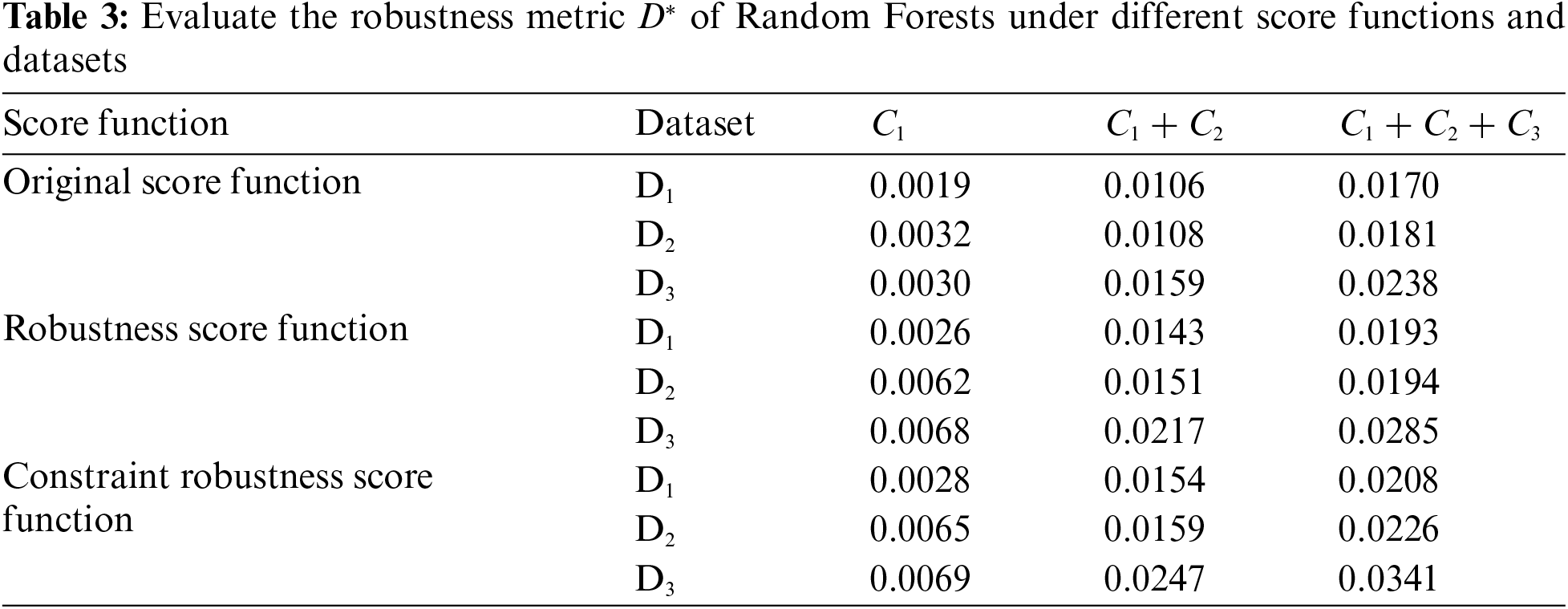
Training with a robustness score function improves robustness across all datasets, with notable enhancements when physical constraints are present. Our results highlight that the robustness score function yields the most significant improvements in robustness when combined with the D3 dataset. This is particularly evident under all constraint conditions (C1 + C2 + C3), where the robustness enhancement is maximized. The introduction of the D3 dataset helps in locally adjusting the decision boundaries of the model. This local adjustment ensures that the model is better equipped to handle adversarial examples that adhere to physical constraints, thereby providing a more precise classification under specific attack scenarios. On the other hand, incorporating a constraint robustness score function provides a global adjustment of the decision boundaries, ensuring that the overall model structure is robust against a wide range of adversarial perturbations. Combining these two approaches—local adjustments from the D3 dataset and global adjustments from the constraint robustness score function—effectively enhances the model’s robustness under physical constraints. This synergistic effect ensures that the generated adversarial examples are realistic and comply with physical laws, thus providing a robust defense mechanism for smart grid applications.

Considering that under physical constraints, some data points cannot generate adversarial examples, we analyzed the robustness metric RP of the tree ensemble-based SSA model. The experimental setup was the same as previously described. As shown in Table 4, with increasing physical constraints, more robust data points can be achieved. The adversarial training method, especially when using the D3 dataset, significantly enhances the proportion of robust data points. Conversely, using the D2 dataset for adversarial training shows minimal impact on RP, indicating the critical role of physical constraints. The use of different score functions also shows limited improvement in RP, particularly without physical constraints. However, the constraint robustness score function provides the most notable enhancements in the presence of physical constraints. This indicates that robust data points arise from the contradictions between the physical constraints and the constraints imposed by adversarial example generation. Both adversarial training methods and different score functions result in limited changes to the model in the absence of physical constraints, explaining the minimal improvement in RP. Furthermore, in the presence of both equality and inequality constraints, the number of points capable of generating adversarial examples is significantly reduced, leading to a limited overall improvement in the RP metric. This demonstrates that the combination of physically constrained adversarial examples and a constraint robustness score function is crucial for achieving higher robustness in real-world applications.

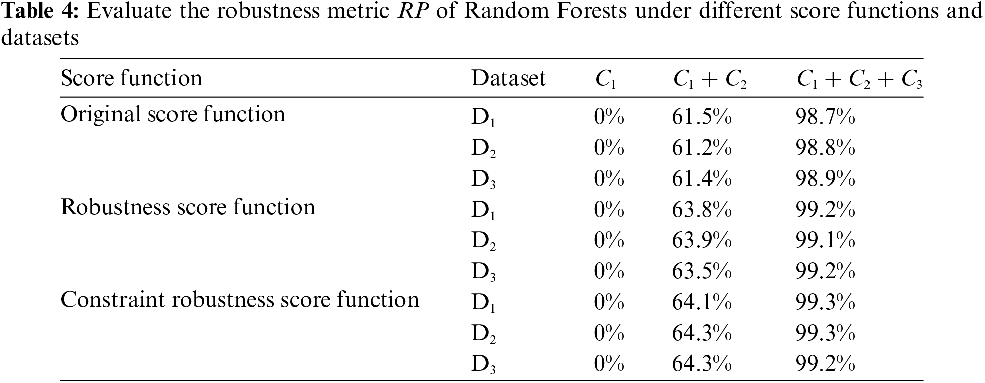
Fig. 2 further illustrates the effectiveness of our approach by comparing the robustness metric D* of Random Forests under different methods and constraints. The comparison involves our method and other robustness enhancement methods that do not consider physical constraints, specifically those by Vos et al. [25] and Chen et al. [26]. The constraints are categorized into three groups: C1, C1 + C2, and C1 + C2 + C3.

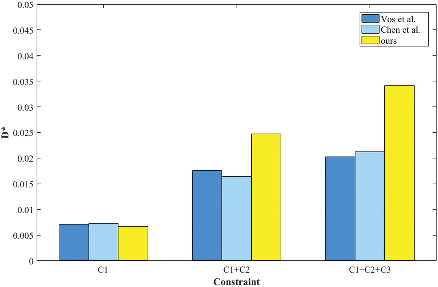
Figure 2: Evaluate the robustness metric D* of Random Forests under different method. Our method is compared with Vos et al. and Chen et al. under different constraints

For the C1 constraint, all three methods show minimal improvement in robustness, with D* values clustered around 0.005. Vos et al. [25] and Chen et al. [26] demonstrate comparable performance, while our method slightly lags behind. As the constraints increase to C1 + C2, the robustness enhancement becomes more pronounced. Here, our method begins to show its strength, surpassing both Vos et al. [25] and Chen et al. [26]. The D* value for our method reaches approximately 0.025, while the other two methods achieve slightly lower values.

Under the most stringent constraints C1 + C2 + C3, our method significantly outperforms the others. The D* value for our method exceeds 0.035, indicating a substantial improvement in robustness. In contrast, Vos et al. [25] and Chen et al. [26] exhibit lower D* values, highlighting the effectiveness of our approach in enhancing model robustness under comprehensive physical constraints.

Overall, the analysis of Fig. 2 demonstrates that our method consistently achieves higher robustness metrics as the complexity of constraints increases, effectively adjusting both locally and globally to enhance the model’s decision boundaries. This confirms the superiority of our method in scenarios with stringent physical constraints, making it particularly suitable for applications in smart grids and other critical infrastructure systems.

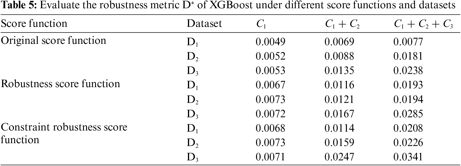
At the same time, we evaluated the robustness of SSA based on XGBoost when model parameters are fixed, under ℓ1 norm. The dataset generation considered unforeseen events T1. From Table 5, it can be observed that the results for the XGBoost model are similar to those for Random Forests. For the XGBoost model, under no physical constraints, the effectiveness of robustness enhancement methods and those considering physical constraints is comparable. However, when inequality constraints are added or when all constraints are considered, the effectiveness of methods considering physical constraints for robustness enhancement surpasses that of general methods. The best results are achieved by combining adversarial training that incorporates physical constraints with score functions that take constraints into account.

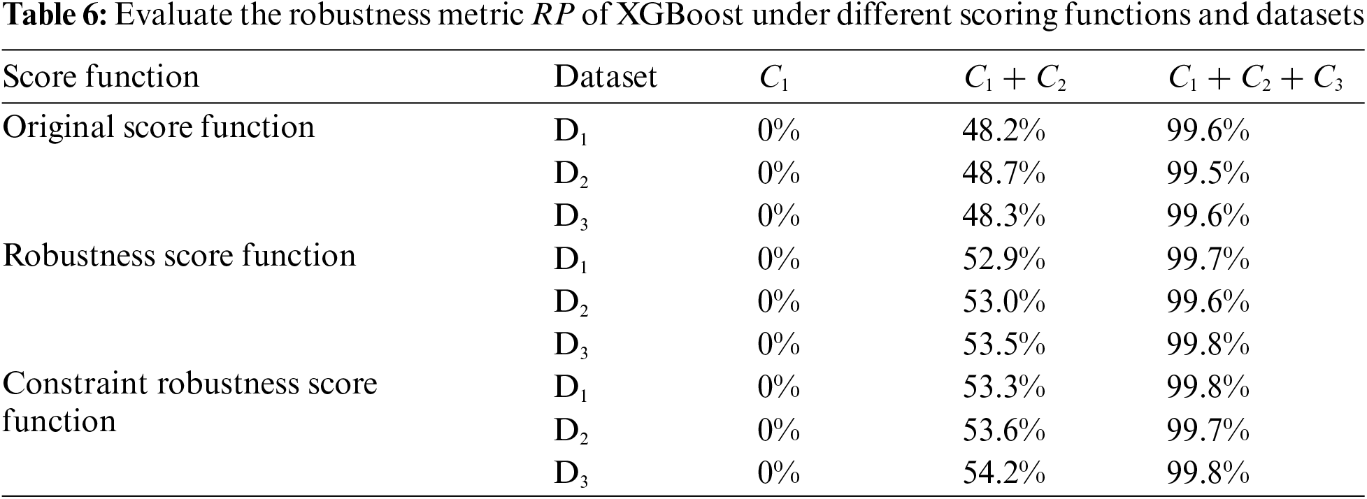
From Table 6, it can be seen that the trend of the proportion of RP for the XGBoost model is similar to that of Random Forests. This trend primarily depends on the physical constraints of the problem, rather than the training method. As the constraint conditions increase, RP significantly improves, reaching close to 100% when all constraints are included. This reflects that in XGBoost, the region of physical constraint and the region of adversarial sample generation mostly do not intersect, leading to an increase in the proportion of robust samples.

In the context of smart grids, the robustness of ensemble tree models is significantly affected by physical constraints. Traditional training methods and unconstrained adversarial training struggle to effectively enhance the models’ ability to withstand adversarial attacks. However, appropriately using physically constrained adversarial examples for adversarial training can significantly enhance the robustness of both Random Forest and XGBoost models under various constraints, which is key to improving the models’ practical application capabilities. Furthermore, the more physical constraints a problem is subjected to, the higher the potential proportion of robust samples, which mainly depends on the nature of the problem itself, not much on the training method. Therefore, when enhancing the robustness of ensemble tree models, it is crucial to fully consider the physical constraints of the actual problem and use adversarial examples that comply with these constraints for training, to truly enhance the models’ robustness. This is vitally important for the safe operation of critical infrastructures like smart grids.

5  Conclusion

This paper proposed a method to enhance the robustness of tree ensemble models in smart grids against adversarial attacks by integrating physical constraints into the training process. The approach involved generating adversarial examples that adhered to physical constraints for adversarial training and modifying feature thresholds to align with these constraints. The experimental results showed a 100% increase in robustness against adversarial attacks. These findings highlighted the potential of the approach to enhance the security and reliability of smart grid applications. Despite the added complexity and computational overhead, the method provided significant benefits for maintaining the integrity of smart grid operations under adversarial conditions. Future work should focus on optimizing computational efficiency and extending this method to other machine learning models and real-world applications. Collaborations with industry partners could facilitate the practical implementation of these robust models in operational smart grids, ensuring their effective and secure operation under adversarial conditions.

Acknowledgement: We express our gratitude to the members of our research group, i.e., Intelligent System Security Lab (ISSLab) of Guizhou University, for their invaluable support and assistance in this research. We also extend our thanks to our university for providing the essential facilities and environment.

Funding Statement: This work was supported by Natural Science Foundation of China (Nos. 62303126, 62362008, 62066006, authors Zhenyong Zhang and Bin Hu, https://www.nsfc.gov.cn/, accessed on 25 July 2024), Guizhou Provincial Science and Technology Projects (No. ZK[2022]149, author Zhenyong Zhang, https://kjt.guizhou.gov.cn/, accessed on 25 July 2024), Guizhou Provincial Research Project (Youth) for Universities (No. [2022]104, author Zhenyong Zhang, https://jyt.guizhou.gov.cn/, accessed on 25 July 2024), GZU Cultivation Project of NSFC (No. [2020]80, author Zhenyong Zhang, https://www.gzu.edu.cn/, accessed on 25 July 2024).

Author Contributions: The authors confirm contribution to the paper as follows: research conception and design: Zhibo Yang; data collection: Zhenyong Zhang; analysis and interpretation of results: Zhibo Yang, Xiaohan Huang, Bin Hu; draft manuscript preparation: Zhibo Yang, Bingdong Wang. All authors reviewed the results and approved the final version of the manuscript.

Availability of Data and Materials: Due to the nature of this research, participants of this study did not agree for their data to be shared publicly, so supporting data is not available.

Ethics Approval: Not applicable.

Conflicts of Interest: The authors declare that they have no conflicts of interest to report regarding the present study.

References

1. Y. Lu, “Cyber physical system (CPS)-based Industry 4.0: A survey,” J. Ind. Integr. Manag., vol. 2, no. 3, pp. 1750014, 2017. doi: 10.1142/S2424862217500142. [Google Scholar] [CrossRef]

2. I. Stojmenovic, “Machine-to-machine communications with in-network data aggregation, processing, and actuation for large-scale cyber-physical systems,” IEEE Internet Things J., vol. 1, no. 2, pp. 122–128, 2014. doi: 10.1109/JIOT.2014.2311693. [Google Scholar] [CrossRef]

3. D. J. Sobajic and Y.-H. Pao, “Artificial neural-net based dynamic security assessment for electric power systems,” IEEE Trans. Power Syst., vol. 4, no. 1, pp. 220–228, 1989. doi: 10.1109/59.32481. [Google Scholar] [CrossRef]

4. R. Eskandarpour and A. Khodaei, “Machine learning based power grid out age prediction in response to extreme events,” IEEE Trans. Power Syst., vol. 32, no. 4, pp. 3315–3316, 2017. doi: 10.1109/TPWRS.2016.2631895. [Google Scholar] [CrossRef]

5. J. R. Vazquez-Canteli and Z. Nagy, “Reinforcement learning for demand response: A review of algorithms and modeling techniques,” Appl. Energy, vol. 235, pp. 1072–1089, 2019. doi: 10.1016/j.apenergy.2018.11.002. [Google Scholar] [CrossRef]

6. G. Apruzzese, M. Andreolini, L. Ferretti, M. Marchetti, and M. Colajanni, “Modeling realistic adversarial attacks against network intrusion detection systems,” Digital Threats: Res. Practice, vol. 3, no. 3, pp. 1–19, 2022. doi: 10.1145/3469659. [Google Scholar] [CrossRef]

7. H. A. Alatwi and A. Aldweesh, “Adversarial black-box attacks against network intrusion detection systems: A survey,” in Proc. 2021 IEEE World AI IoT Congr., Seattle, WA, USA, 2021, pp. 34–40. [Google Scholar]

8. B. Wang et al., “An IoT-enabled stochastic operation management framework for smart grids,” IEEE Trans. Intell. Transp. Syst., vol. 24, no. 1, pp. 1025–1034, Jan. 2023. doi: 10.1109/TITS.2022.3183327. [Google Scholar] [CrossRef]

9. J. Chen et al., “A multi-layer security scheme for mitigating smart grid vulnerability against faults and cyber-attacks,” Appl. Sci., vol. 11, no. 21, pp. 9972, Oct. 2021. doi: 10.3390/app11219972. [Google Scholar] [CrossRef]

10. V. S. Rajkumar, M. Tealane, A. Stefanov, and P. Palensky, “Cyber attacks on protective relays in digital substations and impact analysis,” in Proc. 2020 8th Workshop Model. Simulation Cyber-Phys. Energy Syst., Sydney, NSW, Australia, 2020, pp. 1–6. [Google Scholar]

11. V. S. Rajkumar, M. Tealane, A. Stefanov, A. Presekal, and P. Palensky, “Cyber attacks on power system automation and protection and impact analysis,” in Proc. 2020 IEEE PES Innov. Smart Grid Technol. Europe, The Hague, Netherlands, 2020, pp. 247–254. [Google Scholar]

12. R. Khan, P. Maynard, K. McLaughlin, D. Laverty, and S. Sezer, “Threat analysis of blackenergy malware for synchrophasor based real-time control and monitoring in smart grid,” in Proc. the 4th Int. Symp. ICS & SCADA Cyber Secur. Res. 2016, Swindon, GBR, 2016, pp. 1–11. [Google Scholar]

13. P. Ken et al., “Sandworm Disrupts power in ukraine using a novel attack against operational technology,” 2023. Accessed: Jan. 20, 2024. [Online]. Available: https://cloud.google.com/blog/topics/threat-intelligence/sandworm-disrupts-power-ukraine-operational-technology/ [Google Scholar]

14. G. Burke and J. Fahey, “Israeli hackers cause major disruptions in iranian electricity,” Time News, 2023. Accessed: Jan. 20, 2024. [Online]. Available: https://www.time.news/israeli-hackers-cause-major-disruptions-iniranian-electricity-grid/ [Google Scholar]

15. Z. Zhang, R. Deng, P. Cheng, and Q. Wei, “On feasibility of coordinated time-delay and false data injection attacks on cyber-physical systems,” IEEE Int. Things J., vol. 9, no. 11, pp. 8720–8736, 2021. doi: 10.1109/JIOT.2021.3118065. [Google Scholar] [CrossRef]

16. Z. Zhang, M. Sun, R. Deng, C. Kang, and M.-Y. Chow, “Physics-constrained robustness evaluation of intelligent security assessment for power systems,” IEEE Trans. Power Syst., vol. 38, no. 1, pp. 872–884, Jan. 2023. doi: 10.1109/TPWRS.2022.3169139. [Google Scholar] [CrossRef]

17. X. Zhou et al., “Transient stability assessment based on gated graph neural network with imbalanced data in internet of energy,” IEEE Internet Things J., vol. 9, no. 12, pp. 9320–9331, 2021. doi: 10.1109/JIOT.2021.3127895. [Google Scholar] [CrossRef]

18. K. Morison and M. Glavic, Review of On-Line Dynamic Security Assessment Tools and Techniques. Paris, France: CIGRE, 2007. [Google Scholar]

19. M. Vasconcelos et al., “Online security assessment with load and renewable generation uncertainty: The itesla project approach,” in Proc. 2016 Int. Conf. Probab. Methods Appl. Power Syst., Beijing, China, 2016, pp. 1–8. [Google Scholar]

20. C. Liu et al., “A systematic approach for dynamic security assessment and the corresponding preventive control scheme based on decision trees,” IEEE Trans. Power Syst., vol. 29, no. 2, pp. 717–730, 2013. doi: 10.1109/TPWRS.2013.2283064. [Google Scholar] [CrossRef]

21. A. Madry, A. Makelov, L. Schmidt, D. Tsipras, and A. Vladu, “Towards deep learning models resistant to adversarial attacks,” in Proc. 6th Int. Conf. Learning Representations, Vancouver, BC, Canada, 2018. [Google Scholar]

22. A. Kantchelian, J. D. Tygar, and A. Joseph, “Evasion and hardening of tree ensemble classifiers,” in Proc. 33rd Int. Conf. Int. Conf. Mach. Learning, New York, NY, USA, 2016, vol. 18, pp. 2387–2396. [Google Scholar]

23. C. Szegedy et al., “Intriguing properties of neural networks,” in Proc. 2nd Int. Conf. Learn. Representations, Banff, AB, Canada, 2014. [Google Scholar]

24. H. Chen, H. Zhang, D. Boning, and C. -J. Hsieh, “Robust decision trees against adversarial examples,” in Proc. 36th Int. Conf. Mach. Learning, Long Beach, CA, USA, 2019, vol. 97, pp. 1122–1131. [Google Scholar]

25. D. Vos and S. Verwer, “Efficient training of robust decision trees against adversarial examples,” in Proc. 38th Int. Conf. Mach. Learning, 2022, vol. 139, pp. 10586–10595. [Google Scholar]

26. Y. Chen, S. Wang, W. Jiang, A. Cidon, and S. Jana, “Cost-Aware robust tree ensembles for security applications,” in Proc. 30th USENIX Secur. Sym., 2021, pp. 2291–2308. [Google Scholar]

27. I. Niazazari and H. Livani, “Attack on grid event cause analysis: An adversarial machine learning approach,” in Proc. 2020 IEEE Power & Energy Soc. Innov. Smart Grid Technol. Conf., Washington, DC, USA, 2020, pp. 1–5. [Google Scholar]

28. J. Tian, T. Li, F. Shang, K. Cao, J. Li and M. Ozay, “Adaptive normalized attacks for learning adversarial attacks and defenses in power systems,” in Proc. 2019 IEEE Int. Conf. Commun., Control, Computi. Technol. Smart Grids, Beijing, China, 2019, pp. 1–6. [Google Scholar]

29. J. Tian, B. Wang, J. Li, and Z. Wang, “Adversarial attacks and defense for CNN based power quality recognition in smart grid,” IEEE Trans. Netw. Sci. Eng., vol. 9, no. 2, pp. 807–819, Mar.–Apr. 2022. doi: 10.1109/TNSE.2021.3135565. [Google Scholar] [CrossRef]

30. Z. Zhang et al., “Vulnerability of machine learning approaches applied in IoT-based smart grid: A review,” IEEE Internet Things J., vol. 11, no. 11, pp. 18951–18975, 2024. doi: 10.1109/JIOT.2024.3349381. [Google Scholar] [CrossRef]

31. C. Ren, X. Du, Y. Xu, Q. Song, Y. Liu and R. Tan, “Vulnerability analysis, robustness verification, and mitigation strategy for machine learning-based power system stability assessment model under adversarial examples,” IEEE Trans. Smart Grid, vol. 13, no. 2, pp. 1622–1632, Mar. 2022. doi: 10.1109/TSG.2021.3133604. [Google Scholar] [CrossRef]

32. L. Zeng, D. Qiu, and M. Sun, “Resilience enhancement of multi-agent reinforcement learning-based demand response against adversarial attacks,” Appl. Energy, vol. 324, no. 2, pp. 119688, Oct. 2022. doi: 10.1016/j.apenergy.2022.119688. [Google Scholar] [CrossRef]

33. Z. Zhang, Z. Yang, D. K. Y. Yau, Y. Tian and J. Ma, “Data security of machine learning applied in low-carbon smart grid: A formal model for the physics-constrained robustness,” Appl. Energy, vol. 347, no. 1, pp. 121405, 2023. doi: 10.1016/j.apenergy.2023.121405. [Google Scholar] [CrossRef]

34. L. Zeng, M. Sun, W. Xu, Z. Zhang, R. Deng and Y. Xu, “Physics-constrained vulnerability assessment of deep reinforcement learning-based SCOPF,” IEEE Trans. Power Syst., vol. 38, no. 3, pp. 2690–2704, 2023. doi: 10.1109/TPWRS.2022.3192558. [Google Scholar] [CrossRef]

35. R. D. Zimmerman, C. E. Murillo-Sánchez, and R. J. Thomas, “MATPOWER: Steady-state operations, planning, and analysis tools for power systems research and education,” IEEE Trans. Power Syst., vol. 26, no. 1, pp. 12–19, 2011. doi: 10.1109/TPWRS.2010.2051168. [Google Scholar] [CrossRef]