Dynamic Forecasting of Traffic Event Duration in Istanbul: A Classification Approach with Real-Time Data Integration

1  Introduction

Traffic incidents encompass a variety of events, including traffic accidents, vehicle malfunctions, vehicle fires, and arguments or fights in traffic. These incidents can lead to traffic congestion, which can have significant social, economic, and environmental impacts, such as increased travel time, excessive fuel consumption, air pollution, and stress [1,2]. Predicting the duration of traffic events is a challenging task due to the complexities arising from the stochastic nature of traffic events. Accurate duration prediction offers advantages to drivers in route selection and traffic operations managers in congestion management [3]. Efficient traffic incident management (TIM) is essential for mitigating adverse traffic effects. Continuous enhancement of TIM systems ensures effective incident handling and minimises traffic disruptions. Accurate estimation of event duration, reliant on environmental and event-specific analyses, is pivotal to TIM success. Precise duration estimation informs resource allocation and intervention planning. Diverting affected road users to alternative routes attenuates the incident impact [4].

Forecasting event duration is vital in traffic event management, representing the temporal gap from incident onset to clearance. It is essential for assessing the severity of the incident and determining the temporal and spatial distribution of traffic flow on the road network. Traffic incidents can be divided into sequential and distinct time intervals, as described by several studies [5–8]. The duration between the incident occurrence and the response of the traffic control center operators after receiving the call is known as the detection-reporting time. Preparation-dispatch time is the time between the receipt of the call by the operators and the dispatch of the response team members to the incident. The travel time is simply the duration between receiving the dispatch order and arriving at the scene for the incident response team members. Detection-notification time, preparation-dispatch time, and travel time are three important time intervals in incident response. Clean-up time is the time between the arrival of incident response team members at the scene and the completion of the cleanup of the incident. Clean-up time is especially used in planning and dispatching activities in traffic incident management. In this study, incident duration is defined as the time between the occurrence of the incident and the opening of the roadway.

During traffic incidents, TIM centers first attempt to collect incident coordinates and other relevant information. However, this estimation process is challenging due to the complexity of traffic events and the multitude of variables affecting duration. Uncertainty is inherent at the outset and escalates with incident size. The impact of different factors on incident duration during a traffic event or accident may vary depending on the circumstances, such as partial lane closure, complete road closure, or long-term road infrastructure works. TIMs may make a decision that no intervention is necessary in a low-level traffic incident and then make a similar assessment in a very similar incident that actually requires extensive intervention. Real-time data collection is essential to mitigate assessment errors. Machine learning algorithms are currently the most effective tools in prediction studies of traffic events [9].

Recent studies have focused on predicting traffic incident durations with the objective of enhancing resource allocation, emergency response, and traffic management [10–14]. These studies examine the sub-components of traffic incident durations, such as intervention, and scene cleaning. They utilize various methodologies, including machine learning models, hazard-based modeling, and ensemble learning approaches, in order to improve the accuracy and interpretability of incident duration predictions. Factors influencing incident duration include road type, casualties, weather conditions, and the number of vehicles. The necessity of considering time-varying traffic variables during incident episodes is emphasized, underscoring the importance of dynamic modeling to capture traffic flow dynamics. For real-time forecasting, variables for which real-time data can be collected should be examined and their success in forecasting investigated. The present study proposes an integrated methodology for dynamic estimating traffic incident duration, which addresses a significant gap in existing literature.

The majority of studies employ regression estimation for the purpose of predicting the duration of a traffic event. In contrast, classification is performed in a relatively limited number of studies [15]. In classification studies, the duration of the components of the traffic incident, such as traffic incident notification, response and traffic accident scene cleaning, was studied instead of the total time between the occurrence of the traffic incident and the cleaning of the scene [16]. Unlike previous studies focusing on regression, our novel approach employs classification methods for real-time prediction, reducing the initially examined variables to enhance predictive accuracy. Furthermore, the current study differs from previous research in that it considers the entire period from the occurrence of a traffic accident to the completion of the cleanup, rather than focusing on specific sub-components of traffic incident duration. The present study employs four machine learning methods to categorize traffic accidents and incidents into four duration classes. In order to facilitate dynamic prediction and more effective solutions, we initially reduced the number of variables, which had previously been extensive. Variables that were ineffective in forecasting were eliminated, and it was determined whether the variables that were effective in forecasting could collect real-time data. Subsequently, numerous databases containing the data of these variables were integrated, and a dynamic forecasting environment was provided. The categorization of incident durations and utilization of real-time data enables the swift intervention of incident management centers, fostering agile decision-making and resource allocation compared to conventional regression-based approaches. Feature selection enables the model to improve interpretability while also optimizing training and execution speed, thus mitigating the risk of overfitting. Ultimately, this study provides a pragmatic solution for dynamic traffic incident management, facilitating strategic interventions and resource optimization in urban transportation systems.

An experimental study was conducted in Istanbul to test the model proposed in the study to predict the duration of traffic events. Istanbul is one of the most crowded and traffic-heavy cities in the world, connecting two continents. To create the model, we identified the variables that affect incident duration and collected data from various sources. The objective is to facilitate prompt intervention from the incident management center by estimating the duration of incidents within a given time period using current conditions and primary data with minimal variables. To achieve this, Istanbul was divided into 682 geohash areas. The models were used to forecast the duration of traffic events during specific time period. The model incorporates dynamic prediction through feature selection to streamline complex data structures into fewer variables, facilitating real-time forecasting. Unlike other forecasting approaches, it responds promptly to traffic condition fluctuations by collecting influential variable data in a real-time database. Temporal and spatial considerations enable precise real-time predictions, enhancing the reliability and efficacy of traffic management and emergency response strategies.

The paper is structured as follows: Section 2 reviews prior studies on traffic incident duration, discussing methodologies and models. Section 3 outlines our proposed model, including the dataset, performance metrics, and methods employed. Section 4 presents experimental findings derived from the model. Finally, the concluding section provides objective evaluations of the study and suggests future research directions.

2  Literature Review

The prediction of traffic event duration plays a crucial role in enhancing TIM systems. Prior research has employed diverse regression models and statistical forecasting techniques for forecasting the duration of traffic incidents. Literature suggests that incident delay and duration exhibit variability contingent upon factors encompassing environmental conditions and incident-specific characteristics. Models predicting the duration of traffic incidents are based on various factors, such as incident type, time of day, weather conditions, and traffic volume. These models include regression models [10,15,17], cyclic subspace regression [18], and probabilistic statistical models [19–21]. Hazard-based models were studied by Hojati et al. [1,11,22–24]. Lee et al. [25] analyzed structural equation models, while Zou et al. [26,27] examined finite mixture models. Zou et al. [27] and Laman et al. [16] investigated copula-based models. The literature identifies incident characteristics (e.g., type of incident, first responder, and number of responders), road features (e.g., average annual daily traffic, geometric features, and functional classification), traffic situations (e.g., month, day, and time), and weather conditions (e.g., season, precipitation, temperature, and wind) as the most important independent variables for the developed models.

After a traffic incident, certain information, such as the number of injured individuals, number of vehicles involved, and cause of the accident, may not be immediately available. To improve model accuracy, a dynamic prediction model should be developed gradually using primary data such as the time and location of the incident, incident type, notification time, and weather conditions obtained after the incident notification. Secondary data, encompassing casualty counts, response time, and extent of lane obstruction, may serve as inputs for the initial prediction and subsequent refinement in a two-stage process [28]. Obtaining clear data on the number of fatalities or injuries may take days after the accident has occurred, and the scene may have been cleared during this time, making dynamic forecasting difficult.

Time-series methods can be used to calculate the duration of traffic incidents [29]. Various approaches and techniques, such as genetic algorithms [30], fuzzy logic [31], and Bayesian networks [32,33], can be employed in these models. However, machine learning algorithms have become more preferred over traditional methods in recent years due to the many variables that affect time and the constantly changing traffic conditions. Machine learning models are utilized to predict the duration of traffic incidents by analyzing historical data [9]. These models may undergo training utilising datasets incorporating variables such as the type of event, temporal occurrence, traffic density, meteorological parameters, and event duration. Several machine learning and data mining techniques have been employed to predict the duration of traffic incidents. These models are frequently used in decision trees [34,35], artificial neural networks [9,28], support vector machines [36,37], and random forests [9,12]. Li et al. [38] utilized deep learning in their recent studies. Deep learning, particularly Graph Neural Networks (GNNs), plays a pivotal role in Intelligent Transportation Systems (ITS). GNNs are extensively utilized in ITS applications due to their capacity to analyze graph-structured data effectively. They have evolved for a multitude of ITS tasks, including traffic forecasting, demand prediction, autonomous vehicles, intersection management, and urban planning [39]. Moreover, the integration of deep reinforcement learning (DRL) within connected and automated transportation systems has demonstrated potential in tasks related to automated driving systems and connected-vehicle applications [40]. These advancements in deep learning, including GNNs and DRL, are enhancing the efficiency, safety, and coordination of transportation modes within modern ITS infrastructure, thereby illustrating the potential of data-driven solutions to address complex challenges in the transportation domain.

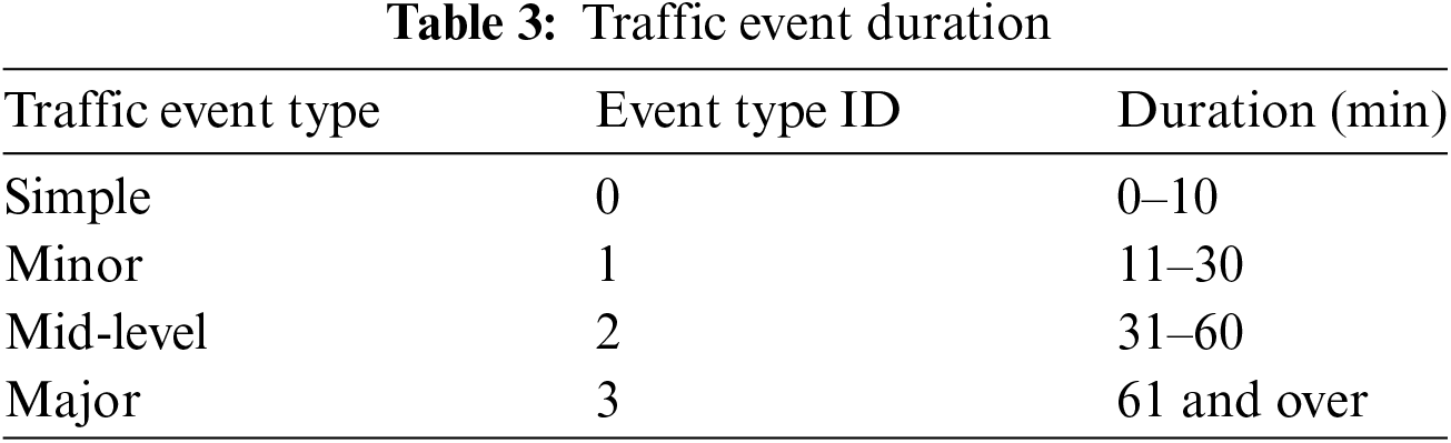
Traffic incident duration can be divided into sequential time intervals, typically two, three, four, or five. Traffic incident durations are classified as either other or severe/major incidents. Lin et al. [41] defined durations as below or above 60 min, while Zhang et al. [42] defined them as below or above 120 min. The triple classification divides tasks into minor/short, medium, and major/long. According to Smith et al. [43], short tasks take less than 15 min, medium tasks take between 15 and 30 min, and long tasks take over 30 min. The US Department of Transportation [44] and Islam [45] define short tasks as taking less than 30 min, medium tasks as taking between 30–120 min, and long tasks as taking over 120 min. In this study traffic event durations were stratified into four distinct categories, delineated according to the frequency of minor events and the implementation of traffic event management protocols. Simple incidents are those that last less than 10 min and do not require intervention. Minor incidents are incidents that require intervention but last between 10 and 30 min, while mid-level incidents last between 31 and 60 min. The study considered incidents that required 61 min or more and a large amount of resources as major incidents.

Recent studies have shown an increase in research on estimating traffic incident duration. Unlike various statistical methods for designing data-driven models, machine learning techniques are frequently utilized and have demonstrated effectiveness [8,38]. These studies have examined the factors that affect incident duration, focusing on individual components of post-event duration, such as notification, response, and cleanup [16]. Our study proposes a model that takes a different approach to estimating traffic event durations. The model employs four machine learning methods and was tested in an experimental study conducted in Istanbul, a large metropolis with complex traffic. The study classified traffic accidents and incidents into four duration classes and estimated their duration based on which duration class the incidents were in. The model simplified the problem by reducing the number of complex features. As a result, instead of extracting data from numerous databases, a few databases were integrated, enabling real-time data for dynamic forecasting.

3  Methodology

This paper presents a model for forecasting the duration of traffic incidents and an experimental study of the model. In this context, the prediction of the duration of traffic incidents is approached as a classification problem rather than a regression problem. The accurate forecasting of the duration of a traffic accident is very difficult, and the specific estimation of the duration is not very useful for traffic management. Instead, knowledge of the accident duration class is much more useful for traffic management. This is because interventions and resources allocated for similar accidents with similar durations of traffic incidents do not differ. The purpose of this study is to manage traffic events and provide resource management by enabling decision-makers to act strategically. This includes determining whether urgent measures need to be taken and directing traffic police based on the duration of the incident in an agile manner. Additionally, reducing the number of features can simplify the model, resulting in faster training and execution, and decreasing the risk of overfitting. This can also improve the model’s ability to generalize and make it more interpretable. It can also prevent resource waste and facilitate effective management by eliminating unnecessary features.

Four machine learning methods were selected for the experimental study: Decision Trees (DT), K-Nearest Neighbors (KNN), Random Forest (RF), and Support Vector Machine (SVM). DT is suitable for modeling simple, non-linear relationships, while KNN excels in classification with easy integration of new data points. RF is chosen for its high performance and robustness, while SVM demonstrates excellent generalization ability and adapts well to high-dimensional data. While other classification methods exist, this study focuses on these four due to their strong performance and general availability, considering factors such as problem requirements and data structure. Furthermore, the combination of databases of variables is employed for real-time prediction. The proposed approach, as illustrated in Fig. 1, allows for the immediate estimation of the duration of traffic incidents.

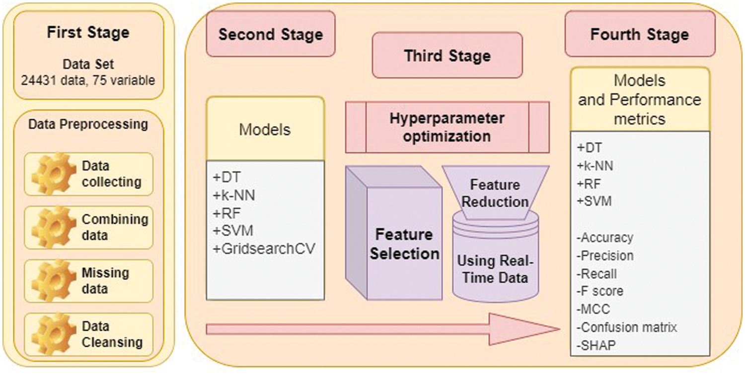
Figure 1: Stages of the proposed approach

The proposed approach for predicting traffic events comprises four distinct stages. The initial stage involves data preprocessing, which is undertaken to refine the dataset for subsequent analysis. The creation of the data set was realized in four steps. In the first step, data was collected with information from nine different open sources or institutions. In the second step, merging was done according to time and location information. In this merging, coordinate information about the location was converted into Geohash codes with ArcGIS. This is because when the coordinates are pointwise, the merging process will be very difficult. In the study, other variables existing in the existing area were integrated thanks to the coordinates converted to a 6-cell geohash area (0.74 km2 area with a cell width of 1.22 km and a cell height of 0.61 km). In this context, it is thought that data merging is rarely done. Missing data were then identified. In cases where missing data were not eliminated, data cleaning was performed, and a data set was prepared to estimate traffic event duration in certain areas. Following this, in the second stage, a non-real-time prediction of the times of the traffic events is carried out using machine learning models. These models leverage the abundance of variables inherent in the initial problem domain. Since this is a critical stage in training four different machine learning models, the hyperparameters must be done carefully. In this context, GridSearchCV was integrated into four different machine learning models and hyperparameters were adjusted. At the same time, the performance of four different machine learning methods was analysed. Subsequently, the complexity of the problem is mitigated through the application of feature reduction and hyperparameter optimization techniques, which facilitate the amalgamation of databases for real-time prediction while refining algorithmic performance. This process culminates in the real-time estimation of traffic event times within a simplified framework, enabling swift and accurate predictions by leveraging optimized algorithms. In this context, feature selection was made with the GridSearchCV algorithm based on the model that gave the best result in the previous stage. In the last stage, with the decreasing number of variables and the real-time data set, the overall prediction of the traffic event duration was dynamically calculated with four different machine learning models. In this context, the performance of the model was compared with the situation in the second stage, and the results obtained from the effective use of resources were evaluated.

3.1 Decision Trees (DT)

DT are a widely used algorithm for classification problem in data mining. They are used to represent classification and regression trees. The advantage of decision trees is their ease of creation and interpretation [46]. The algorithm resembles an upside-down tree, with a structure that extends from the root to sub-branches and new steps that multiply after the sub-branches. Each newly formed branch retains the characteristics of the main branch to which it is connected in the trunk. The data obtained from a selected column in the dataset is applied to the entire tree or dataset [47].

The DT is a classification method that generates a tree structure model composed of decision nodes and leaf nodes based on classification, feature, and target. The feature selection measure provides a ranking for each feature that defines the given training topics and determines which feature will be selected [47]. Measures such as information gain, gain ratio, and Gini index are commonly used in feature selection. Although it is possible to obtain multiple trees from a dataset, the tree with the smallest size is preferred. To terminate the iteration within the decision tree model during variable selection, it is requisite that all constituents within the node are assigned to a singular class. This condition that all elements in the leaves will be in the same class and there will be no values left to classify. Consequently, the iterative process within the decision tree model is halted, culminating in the finalization of the decision tree structure. DT has advantages such as simplicity, interpretability, and flexibility to work with categorical and numerical data. However, it has disadvantages such as bias, tendency to overfitting, and susceptibility to data imbalance.

3.2 Random Forest (RF)

The RF model is an advanced form of the bagging method used for both classification and regression. It is based on two parameters: the number of trees and the number of randomly selected independent variables in each node separation [48]. When creating decision trees, a sample is created using the bootstrap method by replacing as many samples as there are in the original dataset. The RF methodology represents a classification approach that harnesses the collective predictive power of multiple DT to enhance classification accuracy. Prediction outcomes are derived through a process of majority voting, wherein the aggregated predictions of all constituent trees within the forest are considered [3,49]. Critical features of the method include generalization error, parameter adjustment, distance between samples, data imputation, and variable importance, which measures the predictiveness of variables in the decision tree.

RF exhibits proficiency in managing extensive feature sets and demonstrates robust performance even in the presence of missing data. The learning algorithm affords flexibility in generating a predetermined number of trees through the utilization of the “n_estimators” parameter, or alternatively, by employing the “random_state” parameter to introduce randomness in tree selection [3]. In our research, no restrictions were imposed on the number of trees to be created, and no pruning was performed. RF has advantages such as high performance, requiring little hyperparameter tuning, resistance to overfitting, and the ability to handle multiple feature types. However, it has disadvantages, such as the increase in computational cost with the increase in the number of trees.

3.3 K-Nearest Neighbours (KNN)

The KNN algorithm is a non-parametric, memory-based learning classification algorithm. It memorizes training examples for prediction instead of learning a model. The algorithm classifies the k training points (r)r=1,2,…, k closest to a known query point x0 using majority voting among k neighbors. Similarity is defined as the distance between two data points, as measured by a metric [50]. Although the Euclidean distance is the most commonly used metric, other metrics such as Manhattan, Chebyshev, and Hamming distances have also been employed in studies.

The algorithm’s speed is noteworthy as it does not rely on training data sets to make generalizations, keeping the entire training data set in memory during the testing phase. The size of the neighborhood is determined by the k parameter. Setting k to 1 results in low bias but high variance [51]. A k value of 1 means that predictions are made using the single training sample that is closest to the new patterns to be predicted. It is important to note that this prediction method relies heavily on the single closest training sample and may not be as accurate as methods that consider a larger number of training samples. The appropriate k value depends on the size of the data set. In this research, the Manhattan distance metric was selected as the distance parameter due to its capability to accommodate both continuous and categorical variables. While kNN offers advantages such as simplicity, effective classification performance, and easy integration of new data points, it also has disadvantages such as high computational cost, a curse of dimensionality, and sensitivity to noise in the dataset.

3.4 Support Vector Machine (SVM)

The SVM algorithm, originally conceived for binary classification tasks, has undergone adaptation to accommodate both multi-class classification and regression models. Initially constrained to the analysis of continuous variables, SVM has evolved to encompass the examination of categorical variables as well. This expansion entails the automatic conversion of categorical variables into numerical representations, thereby enabling the normalization of both categorical and continuous data within SVM frameworks. The algorithm aims to achieve the most suitable separation between the two classes on the plane. In cases where there are overlapping classes, basic approaches are used to reduce the effects on data points. These include reducing the discriminant margin and reflecting data points into a high-dimensional space using the kernel method, facilitating efficient linear separation. Additionally, the problem can be formulated as a second-order optimization problem at the solution point [52–54].

SVM uses different parameters. The complexity parameter regulates the degree of flexibility exhibited by the decision boundary in class segregation. A setting of 0 mandates strict adherence to the margin, whereas the default value typically stands at 1. Additionally, a crucial parameter to consider is the selection of kernel function. The most elementary among these is the linear kernel, which delineates data instances using a linear decision boundary, often represented as a straight line or hyperplane. The polynomial kernel facilitates the separation of classes by employing a curved or nonlinear decision boundary, the degree of which is contingent upon the exponent value. The radial basis function kernel emerges as a widely adopted and potent alternative, leveraging intricate boundary shapes to effectively segregate classes [52–54]. For this study, default parameters were used, including linear, polynomial, and RBF kernels. SVM has the advantages of good generalisation ability, adaptability to high dimensional data, and flexibility through various kernel functions. However, it has disadvantages such as high computational cost in large data sets and the need for careful tuning of hyperparameters.

3.5 GridSearchCV

GridSearchCV is a hyperparameter optimization method used to determine the best hyperparameters for machine learning algorithms. Exhaustively explores all combinations within a defined set of hyperparameters in pursuit of identifying the optimal values associated with superior performance. This method determines the optimal hyperparameter values by exhaustively testing all combinations in a predetermined set [55,56]. K-fold cross-validation is used for each hyperparameter value, and the results are recorded in a score matrix. The process tests all necessary combinations to obtain the best hyperparameter values [55,57].

3.6 SHAP

Shapley Additive Explanations (SHAP) is a method proposed by Lundberg and Lee in 2017 to evaluate how attributes affect the results. It is an explainability method developed to understand the complexity of machine learning models and explain their prediction results. It can be applied to a wide range of models, from tree-based models to deep learning models, and is an important tool in explainability research. SHAP offers a unique approach to understanding why the model makes a certain prediction and making the model’s decisions more transparent [58].

The SHAP method is based on strong theoretical foundations, making it particularly useful in regulated contexts. It draws on principles from game theory and uses Shapley values to provide specific predictions by assigning importance values (SHAP values) to individual features. These SHAP values adhere to key properties: (1) local accuracy, ensuring the explanation model aligns closely with the original model’s output; (2) missingness, where features absent in the original input have no discernible impact; and (3) consistency, ensuring that increasing dependence on a particular feature in model revisions does not diminish its importance, irrespective of other features [59].

3.7 Performance Matrix

Numerous criteria are employed to evaluate and compare the efficacy of machine learning algorithms. This study evaluates performance using accuracy, precision, recall, Matthews correlation coefficient, F1-score, jaccard and confusion matrix. The confusion matrix is a tool used in machine learning and statistics to measure the performance of a classification model. The confusion matrix is a 2 × 2 matrix that displays four different combinations between actual class and predicted class values: true positive (TP), true negative (TN), false positive (FP), and false negative (FN) [3].

Accuracy shows the percentage of samples classified correctly. The accuracy value ranges from 0 to 1.

Accuracy=(TP+TN)(TP+TN+FP+FN)(1)

Recall indicates the proportion of actual instances of a class that were correctly classified.

Recall=TP(TP+FN)(2)

Precision represents the percentage of samples classified with true labels of a class.

Precision=TP(TP+FP)(3)

F1-score is a measure of the balance between precision and sensitivity, calculated as the weighted average.

F1−score=2∗(Precision∗Recall)(Precision+Recall)(4)

The Matthews correlation coefficient (MCC) is a preferred criterion for evaluating the performance of a classification model or function with two or more classifications. The coefficient takes values between −1 and 1, where −1 indicates reverse classification, 0 indicates average classification performance or poor performance, and 1 indicates perfect classification or prediction [3,60].

MCC=(TP∗TN−FP∗FN)(TP+FP)(TP+FN)(TN+FP)(TN+FN)(5)

4  Experiment and Results

4.1 Data

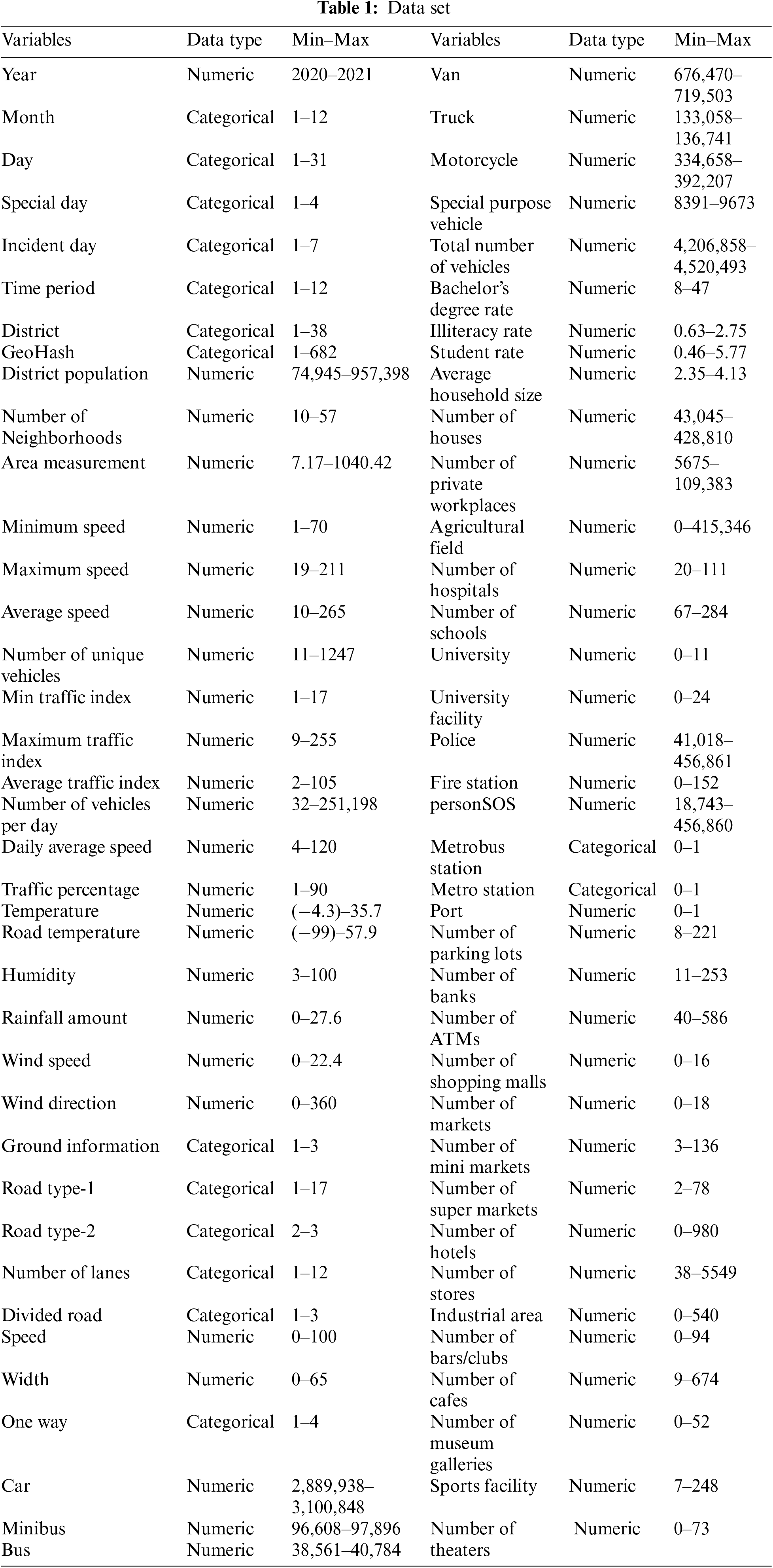
The dataset used in the training process is one of the most important elements of machine learning models. The quality of machine learning models’ predictions is directly dependent on the quality of the training data. Therefore, it is crucial to meticulously collect data that accurately represents the classes targeted by the model. The data set on traffic incidents used in our study was obtained from official institutions, including the Turkish Statistical Institute (TUIK), Istanbul Metropolitan Municipality, the 1st Regional Directorate of Meteorology, and open data portals such as Google Maps, ArcGIS, OpenStreetMap Development Library, and IMM Open Data Portal. The database contains a total of 24,431 records of traffic accidents and incidents, including vehicle breakdowns and fires, that occurred in Istanbul between 2020 and 2021. After collecting the data for analysis, we examined all variables that could impact the prediction. These variables include time, location, vehicle, traffic index, speed, road structure and condition, meteorology, social and demographic factors, and district. Table 1 provides information on the 75 variables and their data types.

4.2 Study Area

Istanbul was chosen for this study because of its cosmopolitan structure and its complex transportation network. The duration of traffic incidents was estimated by considering all locations in the database. The study obtained coordinate-based information on accidents and incidents in Istanbul and used ArcGIS to assign 6th geohash codes to these coordinates. Geohash is a coding system that converts geolocation data into a string and uses it to express the latitude and longitude coordinates of a location in an abbreviated format. Geohash defines a rectangular cell and divides location data into cells. In this way, we attempted to estimate traffic incident duration by performing spatial modeling with geohash areas.

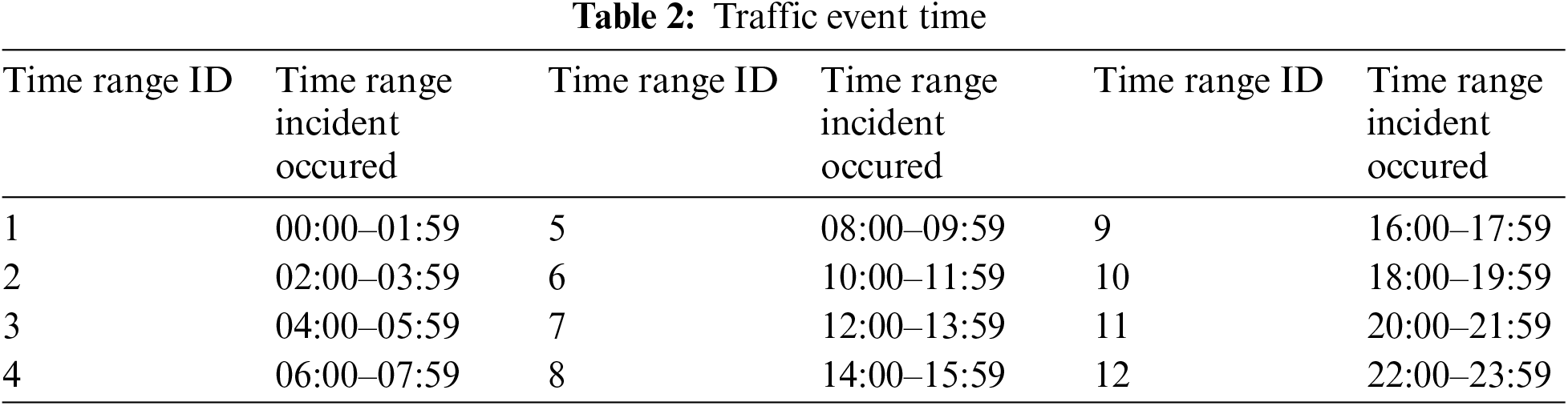
The traffic incident time refers to the moment when a traffic incident takes place. In our study, we divided the 24-h day into 2-h periods, as shown in Table 2, and assigned the start times of traffic events to these segments. This approach aims to detect hidden patterns between events in the same time period and to more accurately predict the duration of a traffic event that may occur during a specific time period.

The literature has established various time intervals for traffic incident duration. To ensure clarity, in our study, four classifications have been made. This is because incidents that last longer than 90 min are rare in Istanbul, while those that last less than 10 min occur more frequently. Simple incidents are those that do not exceed 10 min and typically involve minor vehicle malfunctions or short stoppages. These types of incidents do not require TIM intervention. When examining events that require intervention, it is evident that their duration is between 23 and 31 min at most. Table 3 presents four categories related to the duration of traffic event.

4.3 Setup for the Experiment

The study began with data preprocessing activities. These activities involved combining data from different databases, improving incomplete and noisy data, and obtaining a structured dataset for analysis. To estimate the duration of traffic incidents, the Scikit-learn library was used in the Python program. Four different machine learning models were used: DT, RF, KNN, SVM. The performance of the classification algorithms was then measured. Feature selection was performed, followed by hyperparameter optimization through feature reduction. GridSearchCV was utilized to find the optimal hyperparameter values by testing all combinations within a specified set of hyperparameters. After verifying the feasibility of reduced features, we conducted hyperparameter optimization to evaluate the accuracy of predictions using a real-time database. Experiments were conducted in the Anaconda3 2021.05 environment. A computer with Intel i5 processor, 2.4 GHz, 16 GB RAM and Windows 10 64-bit operating system was used for the experiments.

4.4 Results and Discussions

The experimental study yielded the best results for four different machine learning algorithms when 25% of the test data sets and 75% of the training data sets were used. The performance metrics of the DT, RF, KNN, and SVM models were calculated in terms of accuracy, recall, precision, and F1-score. Table 4 presents the performance of the four models applied.

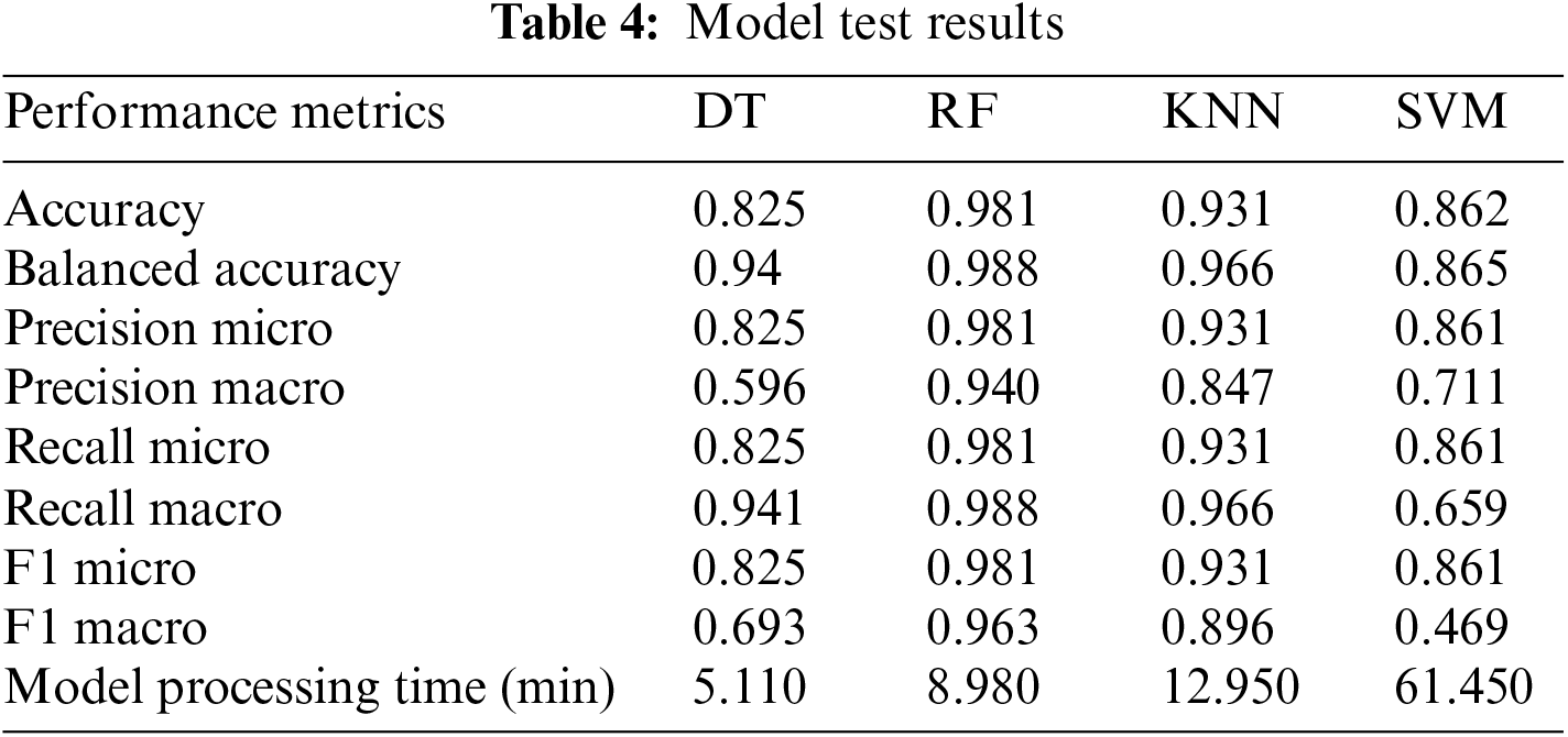
Table 4 displays the accuracy rates for predicting traffic incident duration, with RF achieving the highest rate of 98%, followed closely by other machine learning models such as KNN, SVM, and DT. In terms of precision, both RF and KNN exhibit high precision on both micro and macro scales, while DT shows slightly lower performance. At recall value, both RF and KNN exhibit high success rates on both micro and macro scales. Additionally, both models have high F1-scores on both scales. The fact that the KNN model has the second highest accuracy rate may be due to its ability to effectively recognise similar examples in the data set. The DT model is that they tend to overfit when a single tree is used. The reason why SVM has a low accuracy rate compared to other models may be due to factors such as high computational costs and class imbalances in the data set. While the DT model works with the lowest time, the running times of the KNN and RF models are at an ideal level, and SVM has the highest time values. The unbalanced distribution of traffic events by duration for four traffic event duration classes was a situation that prevented the training dataset from overlearning in the RF model. RF generates a more robust prediction by combining many decision trees together using an ensemble approach. RF requires less precise hyperparameter tuning, making it less susceptible to data instability and noise, resulting in more consistent results.

In our study, ten experiments were conducted in which the data was randomly selected to reduce the randomness of the model due to the selection of training and test samples. Eight evaluation metrics were obtained for each experiment. In order to determine whether there was a significant difference between the DT, RF, KNN, and SVM algorithms used in the study, a normality test was first performed in order to ascertain whether the data was normally distributed. Once it was determined that the data were not normally distributed, the Kruskal-Wallis test with 5% significance level was applied to ascertain whether there was a significant difference in the performance of the methods. The Kruskal-Wallis test evaluates the significance of differences in population medians for a dependent variable across all factor levels. While the null hypothesis (H0) states that there is no significant difference between the methods, the alternative hypothesis (H1) states that there is a significant difference between the methods. Upon examination of Table 5, it can be seen that the value of Sig. (0.000) is less than 0.05, indicating that the null hypothesis is rejected. Results implies that there is a significant difference between the four methods in all performance metrics.

The analysis revealed a correct classification rate of 98%, with a 2% error. However, incorrect predictions were made in some cases, leading to significant differences in performance metrics between classifications. These findings will serve as a valuable reference for future studies in the field. To improve the results, we removed unnecessary variables. Table 4 presents the results obtained from 75 variables using the GridSearchCV algorithm for hyperparameter optimization. The Scikit-learn library was used for optimization, and the GridSearchCV algorithm was employed to cross-validate the models and search for the best parameters. It is important to note that the performance of the models is affected differently by various parameters. Finding the optimal value for each parameter can be computationally expensive. Currently, we have analyzed the parameters that have a greater impact on the outputs. Please refer to Table 6 for the definition of the model parameters. The feature selection process reduced the number of variables from 75 to 14. Table 7 displays the order and weights of the variables selected for the traffic incident duration.

Reducing the number of features from 75 to 14 was a successful outcome in the feature selection phase of the study. This demonstrates the ability of the ML models used to select the most important variables and reduce the complexity of the model, resulting in improved prediction performance. Fewer features allow for more effective predictions with fewer variables. The reduction of features from 75 to 14 indicates that the study’s methodology achieved successful and efficient feature selection. The performances of the algorithms in experiments with 14 variables are given in Table 8. Although the number of variables decreased, there were only minor changes in accuracy rates.

The RF model was found to be the best model, with an accuracy rate increase from 0.981 to 0.985. It has been observed that model processing times are lower with feature reduction. While the RF model’s pre-feature reduction time was 12.95 min, the post-feature reduction time decreased to 7.45 min. This shows that feature reduction increases the speed of the classification process and creates a more efficient and dynamic model. The MCC value of the RF model is 0.864, which means that the model performs very well. This indicates that the model is very good at making correct predictions and has few false predictions. A high value of MCC indicates that the model correctly distinguishes between positive and negative classes. The KNN model also performs well. SVM and DT models show average performance, so these two models have lower performance than the others.

Fig. 2 shows the model’s accuracy results with 75 variables and the accuracy results without using 61 variables with feature reduction. In this context, it was observed that parallel results were obtained for 14 important variables. Since the feature reduction was best achieved with RF, a small improvement was observed, while the accuracy rates of other models showed a small decrease.

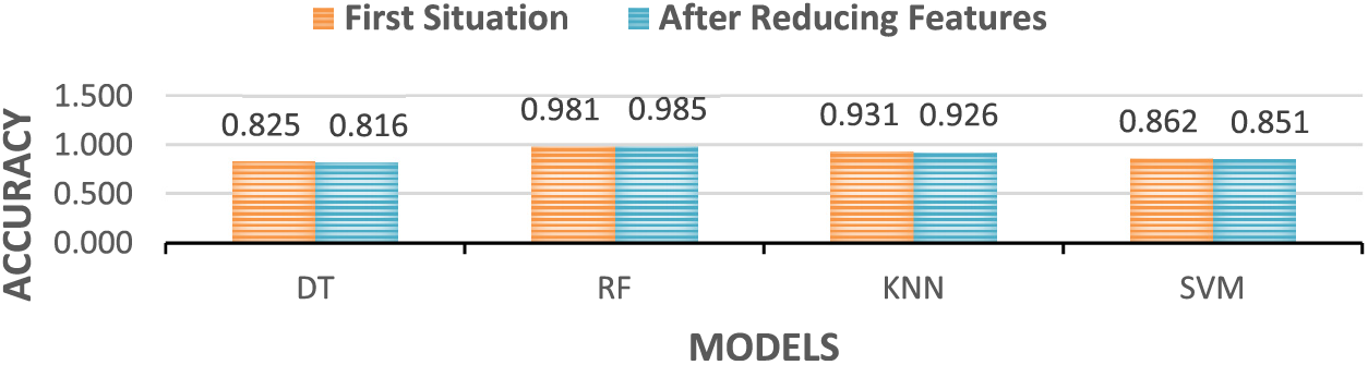
Figure 2: Model results

Fig. 3 displays the complexity matrix of the RF model, which produced the most successful results. The confusion matrix in Fig. 3 includes four different time classes of incident durations. Class 0 represents the intervention time between 0 and 10 min, as shown in Table 3. Class 1 represents a time interval of 11–30 min, and Class 2 represents a time interval of 31–60 min. Class 3 includes events that last more than 61 min. There were 5200 traffic incidents in Class 0 and only 41 in Class 1. First class constitutes 85% of all accident classes. An unbalanced class distribution may cause the model to over-learn. However, the results show that overlearning did not occur. The confusion matrix indicates that the model made correct predictions in 40 out of 41 predictions in the 0th class, 563 out of 566 predictions in the 2nd class, and 322 out of 326 predictions in the 3rd class. The model distinguished between clusters in the data set with an unbalanced distribution. It accurately predicted situations that required emergency intervention and those that did not. The model’s success in classes 0 and 3 indicates its high accuracy. Other metrics also demonstrate the model’s overall success in clearly separating classes without excessive learning.

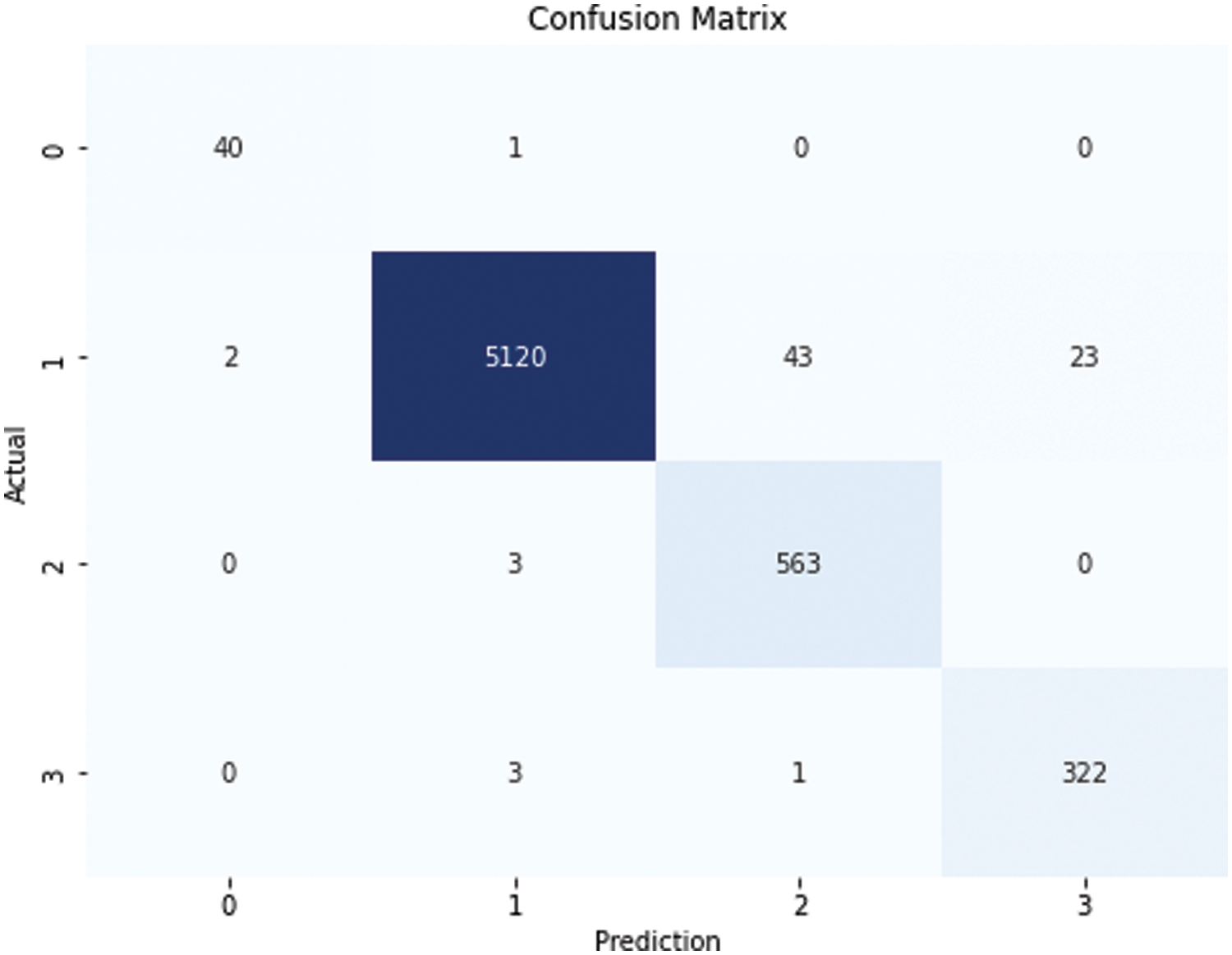
Figure 3: RF confusion matrix

The SHAP method is a mathematical approach based on game theory concepts that is used to explain the predictions of machine learning models. In our study, we used the SHAP method to calculate the contribution of 14 features to the prediction. As a result, we were able to reveal the effects of each feature on the prediction of different classes after the feature reduction phase. Fig. 4 illustrates the influencing rates of 14 independent variables used to predict the duration class of the dependent variable. The time period variable has the most weight in prediction compared to other variables. This means that the time of day when the accident occurs has the greatest impact on the intervention time. Heavy traffic in the city during the daytime is expected to be a priority due to the increased risk of accidents at the beginning and end of work. Response time is also expected to be significantly affected by traffic.

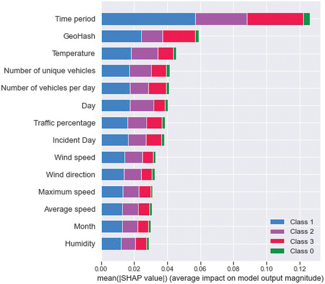
Figure 4: SHAP values

The “GeoHash” attribute is one of the primary variables for all four different classes. While this variable is of secondary importance after the time period in the estimation of 0, 2, and 3 classes, it is in the fourth place after the “Temperature” and “Day” attributes in the estimation of the 11–30 min event durations of Class 1. “GeoHash” provides location information where the accident occurred. It is important to note that the distribution of traffic and accidents on the roads varies due to the non-homogeneous population density in Istanbul. Knowing where the accident took place is crucial information for crime scene intervention, following the time of the accident. Temperature is ranked third in importance for Class 0, second for Class 1, sixth for Class 2, and fifth for Class 3. The study’s use of different time periods and variable weights contributed to the prediction’s accuracy.

5  Conclusion

This study presents a machine learning-based model for forecasting traffic event duration, integrating feature selection and dynamic modeling. Through comprehensive testing, the model reduced 75 variables to 14 significant ones, enabling predictions prior to incidents. Real-time database structuring facilitates dynamic forecasting. The performance evaluations conducted with machine learning algorithms, including DT, RF, KNN, and SVM, revealed that the RF model achieved the highest accuracy and balanced accuracy rates. The model demonstrates effectiveness in traffic incident duration prediction, particularly in complex urban environments, suggesting potential for sustainable prediction systems with reduced variables. Experimental findings underscore its significance for traffic management and planning. We utilized the SHAP technique to identify 14 features that contribute to predictions. The time period holds particular importance for emergency response. Variables such as GeoHash and temperature also significantly influence prediction accuracy across time classes, highlighting the nuanced dynamics of incident duration prediction in urban environments like Istanbul. Each method has its own strengths and weaknesses, highlighting the importance of selecting the appropriate method for a specific problem. RF’s non-parametric nature allows for versatile application across diverse datasets, avoiding rigid assumptions and identifying intricate data patterns. RF minimizes individual tree variations by aggregating predictions from multiple decision trees trained on distinct data subsets, resulting in more accurate predictions through classification voting. Both RF and KNN exhibit high precision, recall, and F1-scores. DT’s performance slightly lags due to potential overfitting with a single tree. Despite its longer runtime, RF is more robust against overlearning from unbalanced data distributions and less sensitive to hyperparameter tuning, resulting in consistently superior predictive performance compared to other models.The RF model’s ability to calculate with 99% accuracy demonstrates its usefulness in dynamic models. It can be executed quickly and efficiently on high-processing computers, making it a valuable tool for managing traffic incidents in cities with high accident rates.

Deep learning and neural networks play a crucial role in predicting the duration of traffic incidents. Various studies have proposed innovative models integrating deep learning techniques such as LSTM, Bi-LSTM, and ANN autoencoders to enhance prediction accuracy. These models leverage features such as traffic flow, incident descriptions, and sensor data [38,40]. The fusion of machine learning with traffic data has shown significant improvements over traditional regression models, achieving up to a 60% accuracy enhancement [40]. Moreover, the interpretability of models such as TabNet has enabled the identification of key factors influencing incident duration, including road type, casualties, weather conditions, and vehicle numbers [61]. These advancements in deep learning models offer valuable insights for efficient resource allocation, emergency response, and traffic management strategies. It is therefore anticipated that even more significant outcomes may be achieved with this proposed approach in future studies as the field of deep learning continues to evolve.

The generalizability of the study can be improved by extending the estimation of traffic incident duration to larger geographical areas. Conducting similar analyses in various regions and countries beyond Istanbul will enable us to gain a broader perspective on the impacts of urban features and traffic infrastructure. Examining various geographic scaling methods can offer a more detailed analysis to determine the most suitable scaling strategy for predicting the duration of traffic events. In this regard, it is crucial to evaluate the impact of geohash scaling and alternative scaling methods. Integrating dynamic factors is essential for the prediction model to better adapt to real-world conditions. With the advent of IoT solutions and smart city applications, traffic event data can now be obtained much faster and independently of human input. By incorporating hard-to-obtain data, the prediction success of the model can be increased, allowing for more effective traffic management strategies and quicker responses to potential issues.

Acknowledgement: Not applicable.

Funding Statement: This research received no external funding.

Author Contributions: Conceptualization, Mesut Ulu; methodology, Mesut Ulu; software, Mesut Ulu, Kenan Mengüç; validation, Yusuf Sait Türkan, Ersin Namlı; formal analysis, Mesut Ulu, Kenan Mengüç; investigation, Mesut Ulu; resources, Tarık Küçükdeniz; data curation, Mesut Ulu, Kenan Mengüç; writing—original draft preparation, Mesut Ulu; writing—review and editing, Yusuf Sait Türkan; visualization, Mesut Ulu, Yusuf Sait Türkan; supervision, Ersin Namlı, Tarık Küçükdeniz and Yusuf Sait Türkan; project administration, Yusuf Sait Türkan, Kenan Mengüç. All authors reviewed the results and approved the final version of the manuscript.

Availability of Data and Materials: Contact the corresponding author if interested in using data.

Conflicts of Interest: The authors declare that they have no conflicts of interest to report regarding the present study.

References

1. A. T. Hojati, L. Ferreira, S. Washington, and P. Charles, “Hazard based models for freeway traffic incident duration,” Acci. Anal. Prev., vol. 52, no. 3, pp. 171–181, 2013. doi: 10.1016/j.aap.2012.12.037. [Google Scholar] [PubMed] [CrossRef]

2. R. Ünlü, “Safer-driving: Application of deep transfer learning to build intelligent transportation systems,” in R. Khaled and A. A. Ella Hassanien, (Eds.The Deep Learning and Big Data for Intelligent Transportation, 1st ed., Egypt: Springer, 2021, vol. 1, pp. 135–150. [Google Scholar]

3. M. Ulu, E. Kilic, and Y. S. Türkan, “Prediction of traffic incident locations with a geohash-based model using machine learning,” Algorithms Appl. Sci., vol. 14, no. 2, pp. 725, 2024. doi: 10.3390/app14020725. [Google Scholar] [CrossRef]

4. A. Saracoglu and H. Ozen, “Estimation of traffic incident duration: A comparative study of decision tree models,” Arab. J. Sci. Eng., vol. 45, no. 10, pp. 8099–8110, 2010. doi: 10.1007/s13369-020-04615-2. [Google Scholar] [CrossRef]

5. D. Nam and F. Mannering, “An exploratory hazard-based analysis of highway incident duration,” Transp. Res. Part A: Policy Pract., vol. 34, no. 2, pp. 85–102, 2000. doi: 10.1016/S0965-8564(98)00065-2. [Google Scholar] [CrossRef]

6. G. Valenti, M. Lelli, and D. Cucina, “A comparative study of models for the incident duration prediction,” Eur. Transp. Res. Rev., vol. 2, no. 2, pp. 103–111, 2010. doi: 10.1007/s12544-010-0031-4. [Google Scholar] [CrossRef]

7. R. Li, “Traffic incident duration analysis and prediction models based on the survival analysis approach,” IET Intell. Transp. Syst., vol. 9, no. 4, pp. 351–358, 2015. doi: 10.1049/iet-its.2014.0036. [Google Scholar] [CrossRef]

8. B. Ghosh and J. Dauwels, “Comparison of different Bayesian methods for estimating error bars with incident duration prediction,” J. Intell. Transp. Syst., vol. 26, no. 4, pp. 420–431, 2022. doi: 10.1080/15472450.2021.1894936. [Google Scholar] [CrossRef]

9. J. Tang et al., “Statistical and machine-learning methods for clearance time prediction of road incidents: A methodology review,” Anal. Methods Accid. Res., vol. 27, no. 3, pp. 100123, 2020. doi: 10.1016/j.amar.2020.100123. [Google Scholar] [CrossRef]

10. A. Garib, A. E. Radwan, and H. Al-Deek, “Estimating magnitude and duration of incident delays,” J. Transp. Eng., vol. 123, no. 6, pp. 459–466, 1997. doi: 10.1061/(ASCE)0733-947X(1997)123:6(459). [Google Scholar] [CrossRef]

11. D. Pan and S. Hamdar, “Prediction of traffic incident duration using: A hazard-based modeling for incident durations extracted through traffic detector data anomaly detection,” Transp. Res. Rec., vol. 2678, no. 2, pp. 389–400, 2024. doi: 10.1177/03611981231174445. [Google Scholar] [CrossRef]

12. H. Zhao et al., “Prediction of traffic incident duration using clustering-based ensemble learning method,” J. Transp. Eng. Part A: Syst., vol. 148, no. 7, pp. 04022044, 2022. doi: 10.1061/JTEPBS.0000688. [Google Scholar] [CrossRef]

13. M. Mumtarin, S. Knickerbocker, T. Litteral, and T. J. S. Wood, “Traffic incident management performance measures: Ranking agencies on roadway clearance time,” J. Transport. Technol., vol. 13, no. 3, pp. 353–368, 2023. doi: 10.4236/jtts.2023.133017. [Google Scholar] [CrossRef]

14. A. Grigorev, A. S. Mihaita, S. Lee, and F. Chen, “Incident duration prediction using a bi-level machine learning framework with outlier removal and intra-extra joint optimization,” Transp. Res. Part C: Emerg. Technol., vol. 141, no. 1, pp. 103721, 2022. doi: 10.1016/j.trc.2022.103721. [Google Scholar] [CrossRef]

15. S. Wang, R. Li, and M. Guo, “Application of nonparametric regression in predicting traffic incident duration,” Transport, vol. 33, no. 1, pp. 22–31, 2018. doi: 10.3846/16484142.2015.1004104. [Google Scholar] [CrossRef]

16. H. Laman, S. Yasmin, and N. Eluru, “Joint modeling of traffic incident duration components (reporting, response, and clearance timeA copula-based approach,” Transp. Res. Rec., vol. 2672, no. 30, pp. 76–89, 2018. doi: 10.1177/0361198118801355. [Google Scholar] [CrossRef]

17. L. Yang, “Clearance time prediction of traffic accidents: A case study in Shandong,” China Australas. J. Disaster Trauma Stud., vol. 26, pp. 185–194, 2022. [Google Scholar]

18. X. Wang, S. Chen, J. Gu, and W. Zhen, “Traffic incident duration analysis based on cyclic subspace regression,” in The ICTE 2013: Safety, Speediness, Intelligence, Low-Carbon, Innovation, USA, 2013, pp. 2854–2860. [Google Scholar]

19. G. Giukiano, “Incident characteristics, frequency, and duration on a high volume urban freeway,” Transp. Res. Part A, vol. 23, no. 5, pp. 387–396, 1989. doi: 10.1016/0191-2607(89)90086-1. [Google Scholar] [CrossRef]

20. R. Li, F. C. Pereira, and M. E. Ben-Akiva, “Competing risks mixture model for traffic incident duration prediction,” Accid. Anal. Prev., vol. 75, no. 6, pp. 192–201, 2015. doi: 10.1016/j.aap.2014.11.023. [Google Scholar] [PubMed] [CrossRef]

21. A. J. Khattak, J. Liu, B. Wali, X. Li, and M. Ng, “Modeling traffic incident duration using quantile regression,” Transp. Res. Rec., vol. 2554, no. 1, pp. 139–148, 2016. doi: 10.3141/2554-15. [Google Scholar] [CrossRef]

22. Y. S. Chung, Y. C. Chiou, and C. H. Lin, “Simultaneous equation modeling of freeway accident duration and lanes blocked,” Anal. Methods Accid. Res., vol. 7, no. 3, pp. 16–28, 2015. doi: 10.1016/j.amar.2015.04.003. [Google Scholar] [CrossRef]

23. L. Lin, Q. Wang, and A. W. Sadek, “A combined M5P tree and hazard-based duration model for predicting urban freeway traffic accident durations,” Accid. Anal. Prev., vol. 91, no. 1, pp. 114–126, 2016. doi: 10.1016/j.aap.2016.03.001. [Google Scholar] [PubMed] [CrossRef]

24. F. Mouhous, D. Aissani, and N. Farhi, “A stochastic risk model for incident occurrences and duration in road networks,” Transportmetrica A: Transp. Sci., vol. 19, no. 3, pp. 2077469, 2023. doi: 10.1080/23249935.2022.2077469. [Google Scholar] [CrossRef]

25. J. Y. Lee, J. H. Chung, and B. Son, “Incident clearance time analysis for Korean freeways using structural equation model,” in Proc. Eastern Asia Soc. Transp. Studies, 2009, Vol. 7, pp. 360. [Google Scholar]

26. Y. Zou, Y. Zhang, and D. Lord, “Analyzing different functional forms of the varying weight parameter for finite mixture of negative binomial regression models,” Anal. Methods Accid. Res., vol. 1, no. 2, pp. 39–52, 2014. doi: 10.1016/j.amar.2013.11.001. [Google Scholar] [CrossRef]

27. Y. Zou, X. Ye, K. Henrickson, J. Tang, and Y. Wang, “Jointly analyzing freeway traffic incident clearance and response time using a copula-based approach,” Transp. Res. Part C: Emerg. Technol., vol. 86, pp. 171–182, 2018. doi: 10.1016/j.trc.2017.11.004. [Google Scholar] [CrossRef]

28. C. H. Wei and Y. Lee, “Sequential forecast of incident duration using artificial neural network models,” Accid. Anal. Prev., vol. 39, no. 5, pp. 944–954, 2007. doi: 10.1016/j.aap.2006.12.017. [Google Scholar] [PubMed] [CrossRef]

29. A. J. Khattak, J. L. Schofer, and M. H. Wang, “A simple time sequential procedure for predicting freeway incident duration,” J. Intell. Transp. Syst., vol. 2, no. 2, pp. 113–138, 1995. doi: 10.1080/10248079508903820. [Google Scholar] [CrossRef]

30. Y. Lee and C. H. Wei, “A computerized feature selection method using genetic algorithms to forecast freeway accident duration times,” Comput. Aided Civ. Infrastruct. Eng., vol. 25, no. 2, pp. 132–148, 2010. doi: 10.1111/j.1467-8667.2009.00626.x. [Google Scholar] [CrossRef]

31. W. Wang, H. Chen, and M. Bell, A study of the characteristics of traffic incident duration on motorways. in Traffic and Transportation Studies, USA: American Society of Civil Engineers (Traffic and Transportation Studies2002, pp. 1101–1108. [Google Scholar]

32. K. Ozbay and E. Noyan, “Estimation of incident clearance times using Bayesian networks approach,” Accid. Anal. Prev., vol. 38, no. 3, pp. 542–555, 2006. doi: 10.1016/j.aap.2005.11.012. [Google Scholar] [PubMed] [CrossRef]

33. H. Park, X. Zhang, and A. Haghani, “ATIS: Interpretation of Bayesian neural network for predicting the duration of detected incidents,” in The 92nd Annu. Meet. Transportation Research Board (TRB 2013), Jan. 2013, pp. 13–17. [Google Scholar]

34. C. Zhan, A. Gan, and M. Hadi, “Prediction of lane clearance time of freeway incidents using the M5P tree algorithm,” IEEE Trans. Intell. Transp. Syst., vol. 12, no. 4, pp. 1549–1557, 2011. doi: 10.1109/TITS.2011.2161634. [Google Scholar] [CrossRef]

35. W. Kim and G. L. Chang, “Development of a hybrid prediction model for freeway incident duration: A case study in Maryland,” Int. J. Intell. Transp. Syst. Res., vol. 10, no. 1, pp. 22–33, 2012. doi: 10.1007/s13177-011-0039-8. [Google Scholar] [CrossRef]

36. J. Lu, S. Chen, W. Wang, and B. Ran, “Automatic traffic incident detection based on nFOIL,” Expert. Syst. Appl., vol. 39, no. 7, pp. 6547–6556, 2012. doi: 10.1016/j.eswa.2011.12.050. [Google Scholar] [CrossRef]

37. K. Hamad, M. A. Khalil, and A. R. Alozi, “Predicting freeway incident duration using machine learning,” Int. J. Intell. Transp. Syst. Res., vol. 18, no. 2, pp. 367–380, 2020. doi: 10.1007/s13177-019-00205-1. [Google Scholar] [CrossRef]

38. H. Li and Y. Li, “A novel explanatory tabular neural network to predicting traffic incident duration using traffic safety big data,” Mathematics, vol. 11, no. 13, pp. 2915, 2023. doi: 10.3390/math11132915. [Google Scholar] [CrossRef]

39. H. Wu, S. Yan, and M. Liu, “Recent advances in graph-based machine learning for applications in smart urban transportation systems,” arXiv preprint arXiv:2306.01282, 2023. [Google Scholar]

40. A. Grigorev, A. S. Mihăiţă, K. Saleh, and M. Piccardi, “Traffic incident duration prediction via a deep learning framework for text description encoding,” in 2022 IEEE 25th Int. Conf. Intell. Transp. Syst. (ITSC), China, Oct. 8–12, 2022, pp. 1770–1777. [Google Scholar]

41. P. W. Lin, N. Zou, and G. L. Chang, “Integration of a discrete choice model and a rule-based system for estimation of incident duration: a case study in Maryland,” in CD-ROM of Proc. 83rd TRB Annu. Meet., Washington, DC, USA, Jan. 2004. [Google Scholar]

42. H. Zhang, Y. Zhang, and A. J. Khattak, “Analysis of large-scale incidents on urban freeways,” Transp. Res. Rec., vol. 2278, no. 1, pp. 74–84, 2012. doi: 10.3141/2278-09. [Google Scholar] [CrossRef]

43. K. Smith and B. L. Smith, “Forecasting the clearance time of freeway accidents,” 2022. Accessed: Feb. 15, 2024. https://rosap.ntl.bts.gov/view/dot/34048 [Google Scholar]

44. US Department of Transportation, Manual on Uniform Traffic Control Devices; For Streets and Highways. Office of Highway Policy Information, US Department of Transportation, Federal Highway Administration, 2009. Accessed: Feb. 15, 2024. [Online]. Available: https://www.fhwa.dot.gov/policyinformation/statistics//2009 [Google Scholar]

45. M. A. Islam, “A literature review on freeway traffic incidents and their impact on traffic operations,” J. Transport. Technol., vol. 9, no. 4, pp. 504–516, 2019. doi: 10.4236/jtts.2019.94032. [Google Scholar] [CrossRef]

46. O. Z. Maimon and L. Rokach, “Data mining with decision trees: Theory and applications,” World Sci., vol. 81, 2014. [Google Scholar]

47. J. R. Quinlan, “Learning decision tree classifiers,” ACM Comput. Surveys, vol. 28, no. 1, pp. 71–72, 1996. doi: 10.1145/234313.234346. [Google Scholar] [CrossRef]

48. L. Breiman, “Random forests,” Mach. Learn., vol. 45, pp. 5–32, 2001. Accessed: Mar. 12, 2024. [Online]. Available: https://link.springer.com/article/10.1023/A:1010933404324. [Google Scholar]

49. S. T. Ikram, V. Priya, B. Anbarasu, X. Cheng, M. R. Ghalib and A. Shankar, “Prediction of IIoT traffic using a modified whale optimization approach integrated with random forest classifier,” J. Supercomput., vol. 78, no. 8, pp. 10725–10756, 2022. doi: 10.1007/s11227-021-04284-4. [Google Scholar] [CrossRef]

50. G. Guo, H. Wang, D. Bell, Y. Bi, and K. Greer, “KNN model-based approach in classification,” in Move Meaningful Internet Syst. 2003: CoopIS, DOA, ODBASE: OTM Confederated Int. Conf. CoopIS, DOA, ODBASE 2003, Catania, Sicily, Italy, Nov. 3–7, 2023. [Google Scholar]

51. H. Trevor, R. Tibshirani, and J. Friedman, “Methods and nearest-neighbors,” in The Elements of Statistical Learning, 1st ed., New York, NY, USA: Springer International Publishing, 2011. Accessed: Mar. 12, 2024. [Online]. Available: https://link.springer.com/book/10.1007/978-0-387-21606-5 [Google Scholar]

52. D. A. Pisner and D. M. Schnyer, “Support vector machine,” in Machine Learning. London: United Kingdom Academic Press, 2020, pp. 101–121. Accessed: Mar. 12, 2024. [Online]. Available: https://www.sciencedirect.com/science/article/abs/pii/B9780128157398000067 [Google Scholar]

53. H. Li, L. Xiong, L. Ohno-Machado, and X. Jiang, “Privacy preserving RBF kernel support vector machine,” Biomed Res. Int., vol. 2014, no. 1, pp. 1–10, 2014. doi: 10.1155/2014/827371. [Google Scholar] [PubMed] [CrossRef]

54. R. Yuan, Z. Li, X. Guan, and L. Xu, “An SVM-based machine learning method for accurate internet traffic classification,” Inf. Syst. Front., vol. 12, no. 2, pp. 149–156, 2010. doi: 10.1007/s10796-008-9131-2. [Google Scholar] [CrossRef]

55. L. Liao, H. Li, W. Shang, and L. Ma, “An empirical study of the impact of hyperparameter tuning and model optimization on the performance properties of deep neural networks,” ACM Trans. Softw. Eng. Methodol., vol. 31, no. 3, pp. 1– 40, 2022. doi: 10.1145/3506695. [Google Scholar] [CrossRef]

56. A. Géron, Hands-on Machine Learning with Scikit-Learn, Keras, and TensorFlow, 2nd ed., Sebastopol, CA, USA: O’Reilly Media, Inc., 2022. [Google Scholar]

57. F. Izhari and H. W. Dhany, “Optimizing urban traffic management through advanced machine learning: A comprehensive study,” J. Intell. Decis. Support Syst., vol. 6, no. 4, pp. 223–230, 2023. [Google Scholar]

58. S. A. Samerei, K. Aghabayk, and A. Montella, “Analyzing pile-up crash severity: Insights from real-time traffic and environmental factors using ensemble machine learning and shapley additive explanations method,” Safety, vol. 10, no. 1, pp. 22, 2024. doi: 10.3390/safety10010022. [Google Scholar] [CrossRef]

59. L. Antwarg, R. M. Miller, B. Shapira, and L. Rokach, “Explaining anomalies detected by autoencoders using shapley additive explanations,” Expert. Syst. Appl., vol. 186, no. 5, pp. 115736, 2021. doi: 10.1016/j.eswa.2021.115736. [Google Scholar] [CrossRef]

60. S. Boughorbel, F. Jarray, and M. El-Anbari, “Optimal classifier for imbalanced data using Matthews correlation coefficient metric,” PLoS One, vol. 12, no. 6, pp. e0177678, 2017. doi: 10.1371/journal.pone.0177678. [Google Scholar] [PubMed] [CrossRef]

61. Q. Shang, T. Xie, and Y. Yu, “Prediction of duration of traffic incidents by hybrid deep learning based on multi-source incomplete data,” Int. J. Environ. Res. Public Health, vol. 19, no. 17, pp. 10903, 2022. doi: 10.3390/ijerph191710903. [Google Scholar] [PubMed] [CrossRef]