A Constrained Local Neighborhood Approach for Efficient Markov Blanket Discovery in Undirected Independent Graphs

1  Introduction

Bayesian network (BN) is a network model that expresses the relationship between random variables and joint probability distributions, which can express and reason about uncertain knowledge [1]. In recent years, BN has been a research hotspot for many scholars, and it has been successfully applied in such areas as fault detection [2,3], risk analysis [4], medical diagnosis [5], and traffic management [6].

In the construction process of BN, the BN structure must first be determined from the given data, and then the network parameters can be continued to be learned [7]. Therefore, studying the structure of BN is the first task that needs to be completed. The current BN structure learning methods can be divided into three types, constraint-based methods [8,9], search-and-score methods [10,11] and hybrid methods [12,13]. Constraint-based methods include Peter and Clark (PC) algorithm [14], Three-Phase Dependency Analysis (TPDA) algorithm [15], etc. Usually, these algorithms start from a fully connected graph or empty graph, and use conditional independence (CI) test to remove as many unwanted edges as possible. The search-and-score method uses a scoring function to measure the optimal structure, such as K2 [16], Bayesian Dirichlet with likelihood equivalence (BDe) [17], Bayesian Information Criterion (BIC) [18], etc., to evaluate each candidate network structure and try to search for the optimal structure that matches the sample data. The method based on the hybrid algorithm combines the two ideas to construct the BN structure. Among them, the role of the constraint-based stage is to construct an undirected independent graph, which is an undirected graph model that can reflect the CI assertion in its corresponding BN structure. The undirected separation characteristics of all node pairs in the undirected independent graph are consistent with the CI relationship between variables in the BN structure.

As shown in Fig. 1, in order to find the CI relationship between node 1 and node 4, it is often necessary to traverse all nodes. That is, use the first-order CI test to calculate the remaining nodes. If no results are found, continue to perform higher order CI tests.

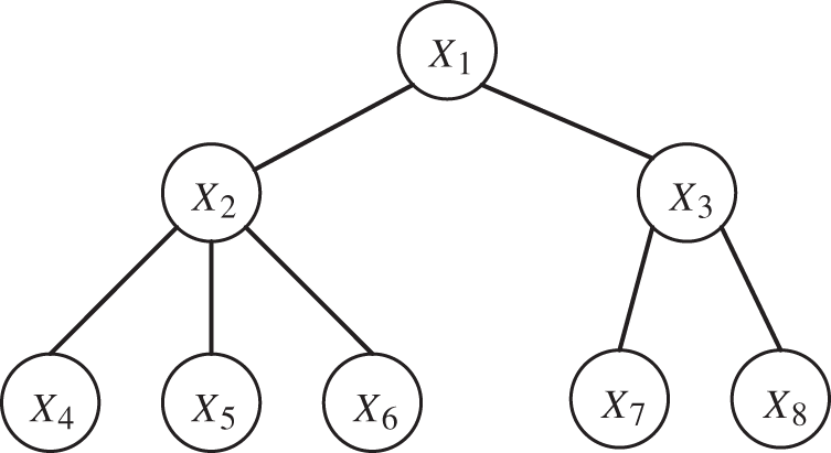
Figure 1: CI test sequence description

It can be seen from the literature that the number of 0-order tests of CI test is Cn2, the computational complexity is O(n2), the number of first-order CI tests is Cn2×Cn−21, the computational complexity is O(n3), and the second-order CI tests are Cn2×Cn−22. the computational complexity is O(n4), so the lower the order and the fewer the number of calls, the better when calculating the CI test. However, how to find node 2 quickly and accurately, and perform the CI test first, is an urgent problem to be solved. Through graph observation, it can be found that the nodes are generally adjacent to each other and the distance from the calculated node is relatively short. Therefore, in order to improve the execution efficiency of the algorithm and reduce unnecessary computational consumption, a reasonable approach is to start from the local constraints of the nodes to be calculated and lock the inspection scope as soon as possible.

Without prior knowledge, using existing methods to construct undirected independent graphs is a huge challenge in terms of time complexity or space complexity. Spirtes first proposed the classic Spirtes, Glymour and Scheines (SGS) algorithm [19], which uses the CI between nodes to determine the network structure when the order of the nodes is unknown. However, the operating efficiency of this method is too slow, and the number of CI tests that need to be carried out is exponential. Subsequently, through improvement, the PC algorithm [20] was proposed. The algorithm started from a completely undirected graph, and then passed the low-order CI test to reduce the number of edges. After that, the segmentation set is searched from adjacent nodes, thereby reducing the time complexity and the number of calls for high-order independence tests. However, because this method uses randomly selected constraint sets to calculate the CI test between nodes, there are many uncertainties and excessive randomness.

On this basis, some scholars have proposed to improve the sorting method [21] or independent method [22] to solve the random problem in the PC algorithm. The order of independent testing of nodes has no corresponding constraints. This makes the test process randomly and cannot generate candidate structure well. However, although this kind of method alleviates the problem of false negative nodes to a certain extent. It cannot solve the problem of false positive nodes or the exponential problem of the number of inspections.

Later, Cheng et al. [23] proposed a three-stage analysis algorithm TPDA based on mutual information. This method uses the mutual information between nodes to obtain an initial network structure. However, this method needs to use the known node sequence for structural learning, and over-relies on the index of mutual information, which makes the learning accuracy and learning efficiency decrease. Xie et al. [24] innovatively proposed a recursive algorithm to gradually reduce the conditional independence test set to the minimum condition set, and finally combine the obtained local results. However, as the number of vertices in the network increases, finding the variables that split the set becomes more complex, and there are inherent weaknesses in CI testing. Literature [25] was based on the Max-Min Hill-Climbing (MMHC) algorithm and uses a heuristic strategy to obtain an undirected independent graph. This method performs a CI test on all elements in the obtained candidate parents and children (CPC). The effects of high-level independence tests, exponential tests, and variable order still restrict the performance of existing algorithms. Therefore, some scholars proposed to construct the initial undirected independent graph based on Markov blanket method. Guo et al. proposed the dual-correction-strategy-based MB learning (DCMB) algorithm [26] to address the issue of false positives and false negatives that may arise during simultaneous correction of CI tests. The algorithm utilizes both “and” and “or” rules to correct errors, demonstrating advantages in handling noisy and small-sample data.

Wang et al. [27] proposed an efficient Markov discovery algorithm efficient and effective Markov blanket (EEMB) discovery algorithm, which consists of two phases: a growing phase and a shrinking phase. Although the algorithm can get Markov blanket efficiently and quickly, it still needs a large number of CI tests in the calculation phase. There is no effective reduction of the number and order of the independent testing of the independent test. Researchers have proposed the Error-Aware Markov Blanket (EAMB) algorithm [28], which comprises two novel subroutines: Efficiently Simultaneous MB (ESMB) and Selectively Recover MB (SRMB). ESMB is aimed at enhancing the computational efficiency of EAMB while minimizing unreliable CI tests as much as possible. SRMB adopts a selective strategy to address the issue of unreliable CI tests caused by low data efficiency. Experimental results have demonstrated the rationality of the selection strategy. However, the algorithm relies on parameter settings.

It can be seen from the above references that constraint-based algorithms need to quickly and accurately obtain the constraint space in the early stage of the algorithm. Most algorithms use global node information to constrain, ignoring the unique local neighborhood relationship between nodes. At the same time, excessive dependency testing will consume more computing resources, resulting in low algorithm efficiency. In particular, a large number of high-order CI tests have significantly increased the complexity of the algorithm. Above on this, we proposed a Markov blanket discovery algorithm for constraining local neighborhoods. The algorithm first finds the local neighborhood space of the node accurately by setting the constraint radius, and completes the initialization of the constraints. After that, the establishment of Markov blanket constraint space was completed through low-level CI test, and then the construction of undirected independent graph in BN structure learning was completed. Specifically, the main contributions of this article are as follows:

•   Firstly, the initial search space is quickly determined by leveraging the dependencies between nodes. Subsequently, the local neighborhood of nodes is constrained by an inter-node constraint radius r to reduce the computational cost of the subsequent algorithm.

•   Secondly, to decrease the complexity of the CI tests, the Markov blanket discovery algorithm is employed to further refine the set of nodes within the constrained local neighborhood, thereby continuing to reduce the search space.

•   Finally, low-order CI tests are used to update the Markov blanket set, ensuring the inclusion of correct connected edges in the set and generating an undirected independent graph that accurately represents these connections.

The method proposed in this paper not only uses constraint knowledge to compress the search space, but also limits the structure search space quickly and accurately, while reducing the order of CI tests and the number of CI tests. The advantages of the algorithm are verified through comparative experiments with other algorithms.

The rest of this paper is organized as follows: Section 2 discusses related work. Section 3 presents the proposed algorithm. Section 4 discusses the experimental results, and Section 5 concludes the paper and future work.

2  Preliminaries

The BN consists of a two-element array, namely BN=(G,T). Where G=(V,E) is the directed acyclic graph of the BN network structure, and V is the set of nodes in the network, that is V={x1,x2,⋅⋅⋅xn}, E is the set of directed edges in the network.

2.1 Markov Blanket

In the complete set U of random variables, if X∉U and U are the smallest set satisfying the following conditions:

(X⊥X−{X}−U|U)∈Γ(P)(1)

Then call U the Markov blanket of X in distribution P, denoted by MB(X).

In the complete set U of random variables, given a graph G, the Markov blanket of X in graph G is MB(X), for a given variable X∈U and variable set MB⊂U(X∉MB), if there is:

X⊥{U−MB(X)−{X}}|MB(X)(2)

Then it is said that the minimum variable set MB that can meet the above conditions is the Markov blanket of X, that is, when the set MB is given, X and other nodes in the graph are independent of each other. It can be proved that these local independence assumptions are factorized on the graph G Any distribution of is established. When using the Markov blanket discovery algorithm, the purpose is to quickly find the Markov blanket of the required variables in the full set, shrink the redundancy of the global information, and reduce the dimension of the feature space.

2.2 Mutual Information

Mutual information MI(X,Y) can quickly detect the dependence relationship between random variables, which can be used to measure the dependence relationship between random variables. And the mutual information value between the random variables is positively correlated with the degree of dependence between the random variables. That is, the higher the degree of dependence between the random variables X and Y, the greater the mutual information value. There is a directly connected edge or an indirectly connected edge between the two. Conversely, if the mutual information value between X and Y is small, it means that the two nodes have a low degree of dependence, which is reflected in the network structure. That is, X and Y are conditionally independent of each other, and there is no connecting edge between the two. It can be expressed as:

MI(X,Y)=∑X∑YP(X,Y)log2⁡P(X,Y)P(X)P(Y)(3)

where P(X,Y) is currently the joint probability density function of X and Y, and P(X) and P(Y) are the marginal probability density functions of X and Y, respectively.

Suppose X, Y, Z are three disjoint variable sets, then under the condition of given Z, the mutual information of X, Y is:

MI(X,Y|Z)=∑X∑Y∑ZP(X,Y,Z)log2⁡P(X,Y,Z)P(X|Z)P(Y|Z)(4)

Therefore, mutual information is used to judge the connectivity between every two nodes in the network. Since mutual information has symmetry, that is MI(X,Y)=MI(Y,X), the network structure composed of mutual information is undirected.

2.3 Conditional Independence Test

Assuming that X, Y, and Z are three independent sets of random variables, if

P(x∈X,y∈Y)=P(x∈X)P(y∈Y)(5)

It is said that variables X and Y are conditionally independent, that is X⫫Y.

Given the variable Z, if

P(x∈X,y∈Y|z∈Z)=P(x∈X|z∈Z)P(y∈Y|z∈Z)(6)

It is said that under the condition of a given Z, X and Y are conditionally independent, expressed as Ind(X,Y|Z), or X⫫Y|Z.

When testing the CI of nodes X and Y, it is necessary to find a constraint set Z to make the above formula true, but it is often difficult to achieve in the search process.

3  Markov Blanket Discovery Algorithm for Undirected Independent Graph Construction

In the process of constructing BN undirected independent graphs, the local neighborhood topology information of nodes is more often ignored, which makes excessive use of CI tests to constrain nodes. Moreover, the excessive randomness of selecting nodes also greatly increases the computational cost. Therefore, in order to improve calculation efficiency and calculation accuracy, we proposed a Markov blanket discovery algorithm for constrain local neighborhoods. Avoid blindly using the CI test, and use the local neighborhood information between nodes to constrain it. And use the Markov blanket discovery algorithm to further reduce the search space. Finally use fewer low-level CI tests to complete the construction of the undirected independent graph. The specific algorithm is implemented as follows:

3.1 Algorithm Initialization

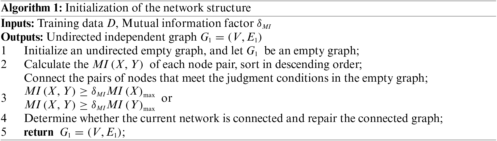
In the process of constructing independent graphs using Markov blanket algorithm, since the number of Markov covering elements increases exponentially with the increase of the number of nodes, it is necessary to constrain the initial structure of the network. The algorithm initialization starts from an undirected empty graph, and first needs to calculate the mutual information value of all nodes. Use the mutual information value to judge the relationship between each node, thereby introducing the local constraint factor δMI. Connect the edges that meet the judgment conditions to establish a constrained initial Markov blanket model, and use the following equation to judge the dependency of the node pair:

MI(X,Y)≥δMIMI(X)maxorMI(X,Y)≥δMIMI(Y)max(7)

where 0≤δ≤1 represents the threshold value that restricts the use of mutual information in the network to determine the strength of dependence between nodes. MI(X)max and MI(Y)max represent the maximum mutual information values between node X and node Y and other nodes, respectively.

It can be seen from the above equation that the restriction of the initial model can be completed by setting the restriction factor δMI. When the constraint factor δMI is small, the number of node pairs under this constraint is small. However, there are more pairs of nodes with strong dependence, and at this time, the two nodes are connected by an edge. When the constraint factor value is larger, there are more node pairs in the network structure that satisfy the constraint model, but there are more node pairs with weak dependency at this time, and no connection is made at this time. After completing the above steps, an initial network structure with local constraints is established. The following Algorithm 1 shows the construction process of the initial network structure:

The network structure of the BN is generally a connected graph. After the above construction process, an undirected graph may appear in the middle link, which may be disconnected. Therefore, the connectivity of the undirected graph needs to be repaired. It can be known from graph theory that if an undirected graph is a non-connected graph, the undirected graph can be represented by several connected components. Only by ensuring that these connected components are connected to each other, the unconnected graph can be restored to a connected graph. Therefore, it is necessary to repair the connectivity of the current network after the mutual information value is judged.

It can be seen that the current undirected graph network is only established under the condition of mutual information. If the accuracy of its judgment is further increased, the Markov blanket needs to be corrected twice by other means.

3.2 Markov Blanket Discovery Algorithm

After the completion of the network initialization and construction in the previous stage, using mutual information value constraint judgment, more edges are added to the empty graph, and because the constraint factor δMI is relatively loose, the undirected independent graph construction process may introduce more edges. Many false positives connect edges.

As a result, in the second phase of the algorithm, through the local characteristic information between nodes and the CI test, the false positive connection edges are eliminated, and the potential missing edges are found, and finally a Markov blanket with higher accuracy is established. Therefore, in this phase, we will conduct two CI tests.

As mentioned in the previous chapter, when there is a connection between two nodes, the CI test accuracy of adjacent nodes is relatively high, and the amount of calculation is low. In order to reduce the number of invocations of the CI test and reduce the computational cost, the neighboring nodes should be used first to perform the CI test. For this reason, a constraint radius r is introduced, that is, when the distance between two nodes is less than r, we believe that the mutual verification relationship between the nodes is more reliable. When the distance between two nodes is longer than r, the connection relationship between the two nodes is not considered, and the CI test is not performed, which will greatly reduce the calculation cost and improve the calculation efficiency.

r=ln⁡(n+ne)2(8)

where n is the number of nodes in the network, and ne is the number of connected edges in the existing network.

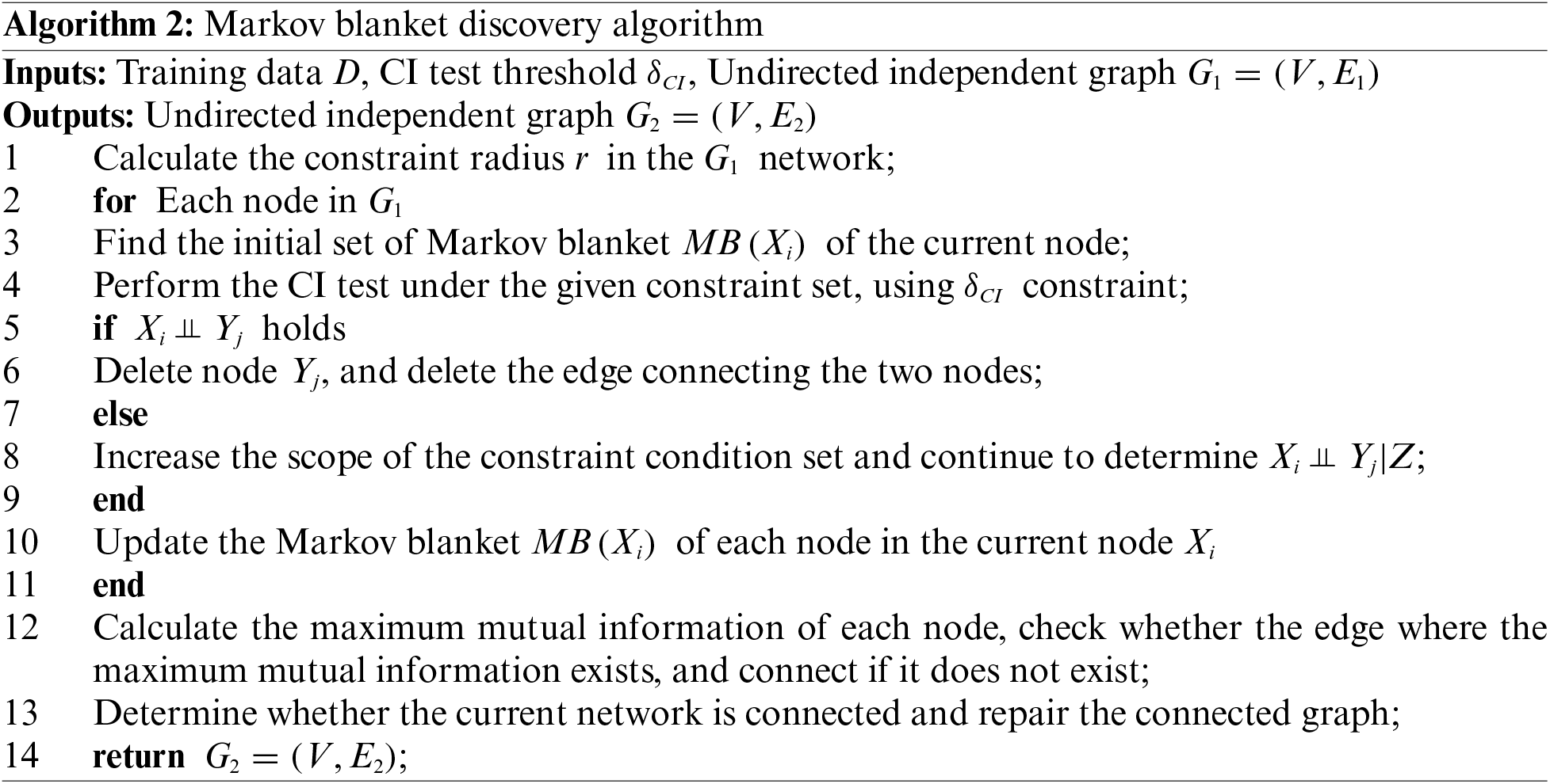
Using the calculated constraint radius r and candidate test node selection rules, the initial set of Markov blanket set based on local constraints is first generated. In order to reduce the number of CI test calls, after the Markov cover set is established, the conditional independence of node X and node Y is detected from the empty set of the constraint set. If it is not true, then select the constraint set from the initial set, and gradually increase the size of the constraint set. If the conditions of node X and node Y are established independently, the connecting edge between the two nodes is deleted, and the node is deleted from the initial set of Markov blanket, otherwise the subsequent procedures are continued. At this point, the initial Markov blanket set can be obtained through the above operations. The specific implementation process of the algorithm (Algorithm 2) is as follows:

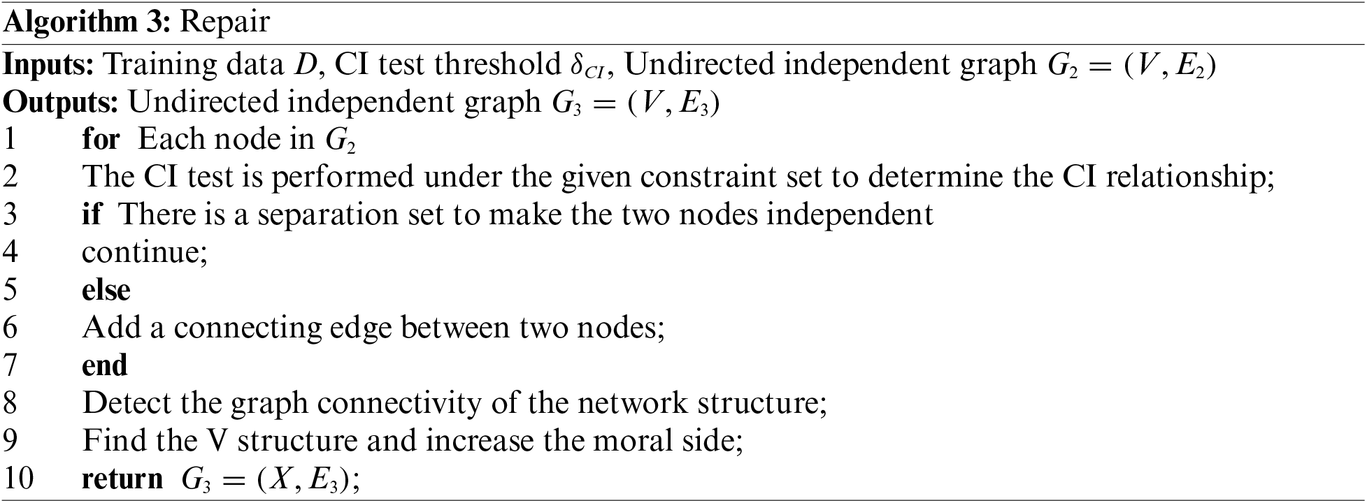
In order to prevent the false deletion of true positive connected edges after the second step of the algorithm is executed. That is, some missing nodes are not added to the Markov cover set, and to avoid the possibility of incompletely connected graphs in the current graph model. Therefore, the last part of the algorithm fixes this problem. First, reconfirm its connectivity and repair it, and secondly, continue to use reliable CI tests to complete this part. On the basis of obtaining the undirected graph of the second step algorithm, use CI to test the independence relationship between computing nodes, and correct the nodes in the Markov blanket set. In particular, this part of the adjustment will no longer delete edges. Finally, we can get a complete connected undirected independent graph G3=(V,E3). The specific implementation process of the algorithm (Algorithm 3) is as follows:

3.3 The Time Complexity of Algorithm

In this section, we will analyze the time complexity of the algorithm, and use the worst-case time complexity as the basis for judgment. Next, we will discuss the time complexity of each step separately. Assuming there are n nodes and the size of dataset D is m.

In Algorithm 1, we first initialize the network structure, which has a time complexity of O(1). Next, we calculate the MI for each pair of nodes. This requires computing MI values for n(n−1)/2 pairs of nodes, resulting in a total time complexity of O(n2×m).

In Algorithm 2, the initial calculation of the constraint radius r has a time complexity O(1). Iterate through each node in the graph G to find the initial MB(X) for the current node has a time complexity of O(n×m). Perform CI tests under the given constraints: Test each neighbor of every node, resulting in a time complexity of O(n×m). Update the MB(X) for each node: The time complexity is O(n×m). Compute the maximum MI for each node and check for edges with maximum MI: The time complexity is O(n2×m). Check if the current network is connected and repair the connected components if necessary: The time complexity is O(n). Therefore, the total time complexity of the algorithm is O(n2×m).

In Algorithm 3, there are steps similar to those in Algorithms 1 and 2. The most time-consuming step is the CI tests, which have a time complexity of O(n2×m). Therefore, the overall time complexity of the algorithm is O(n2×m).

4  Experimental

In order to verify the performance of this algorithm, the experiment is divided into two parts in total. The first part determines the value of the algorithm parameters, and uses the comparison of various indicators under different data sets to determine the generalization of specific parameters. The second part brings the parameter calculation results into the subsequent process, and compares it with the other three similar Markov blanket algorithms to verify the effectiveness of the algorithm. The experimental platform used in our paper is a personal computer with Intel Core i7-6500U, 2.50 GHz, 64-bit architecture, 8 GB RAM memory and under Windows 10. The programs are all compiled using the MATLAB software release R2014a.

4.1 Algorithm Parameter Determination

In order to verify the two parameters δMI and δCI mentioned in the algorithm, the experiment set the parameters to different values, and the parameters were determined by comparing different indexes.

Parameter experiment setting range, δMI is 0.1 step length each time, increasing from 0.2 to 0.9; δCI is 0.03 step length each time, increasing from 0.01 to 0.35. As there will be four different situations in the forecasting process, see Table 1 for details.

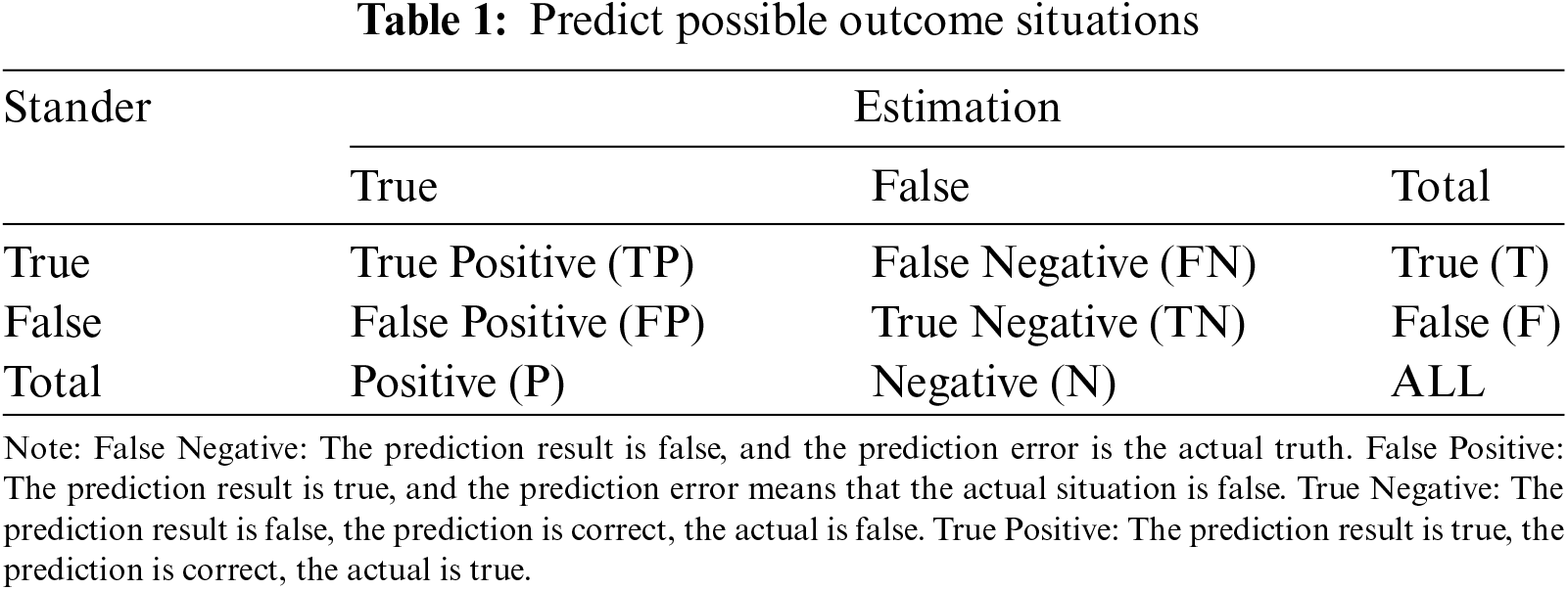
This article uses the following four indicators to determine the performance of the experiment [29]:

Accuracy:

ACC=(TP+TN)/(P+N)=(TP+TN)/ALL(9)

Euclid Distance:

ED=(1−TPR)2+(1−FPR)2(10)

True positive rate: Sometimes called sensitivity

TPR=TP/(TP+FN)=TP/T(11)

False positive rate: Sometimes called specificity

FPR=FP/(FP+TN)=FP/F(12)

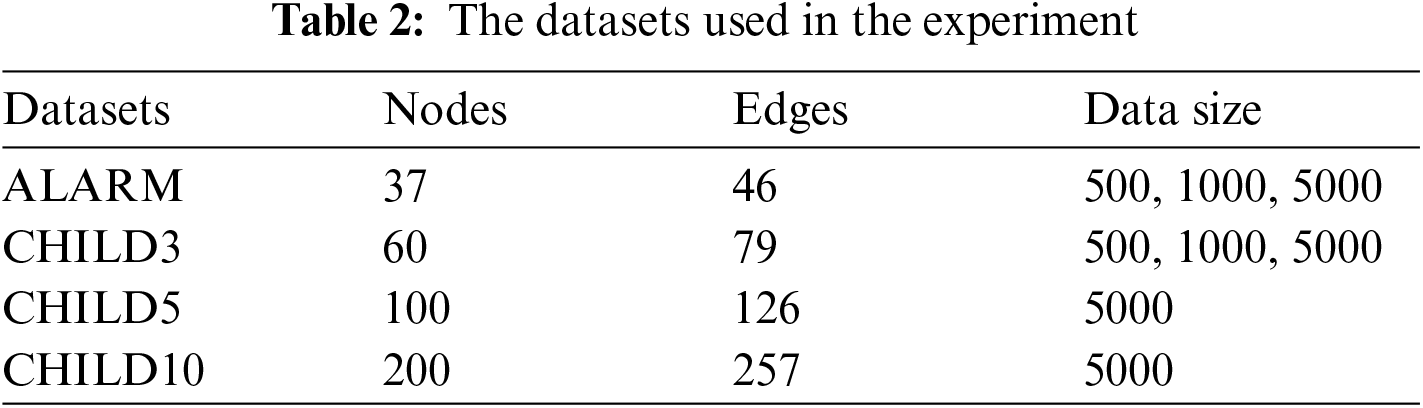
The experiment uses 6 different sample data of four standard data sets, namely AMARM network, CHILD3 network, CHILD5 network and CHILD10 network, each network has 500, 1000 or 5000 sets of data. The specific information of the data is shown in Table 2.

The horizontal axis of the experimental results represents the results corresponding to different parameter values of δMI, and the vertical axis represents the results corresponding to different parameter values of δCI. Each evaluation index is distinguished by the color value. The specific experimental results are shown in Figs. 2–9.

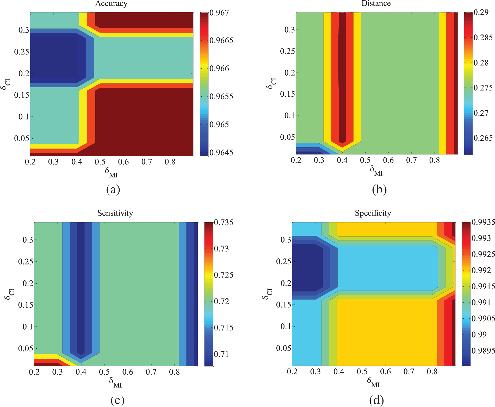
Figure 2: ALARM-500 data set parameter changes. (a) Accuracy; (b) Euclid Distance; (c) True positive rate; (d) False positive rate

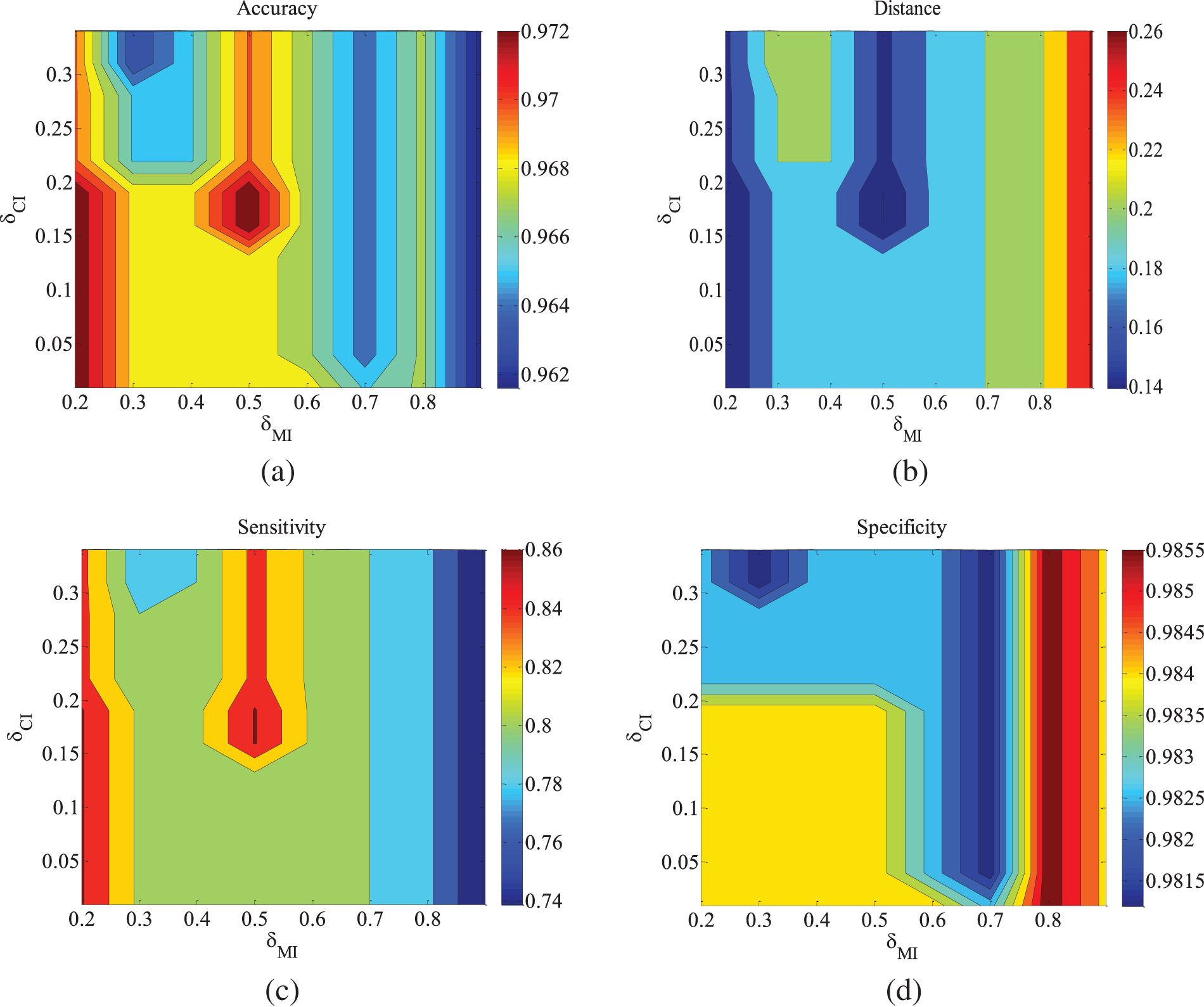
Figure 3: ALARM-1000 data set parameter changes. (a) Accuracy; (b) Euclid Distance; (c) True positive rate; (d) False positive rate

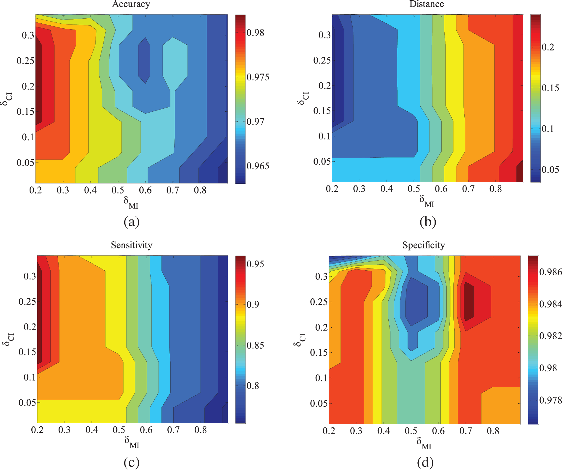
Figure 4: ALARM-5000 data set parameter changes. (a) Accuracy; (b) Euclid Distance; (c) True positive rate; (d) False positive rate

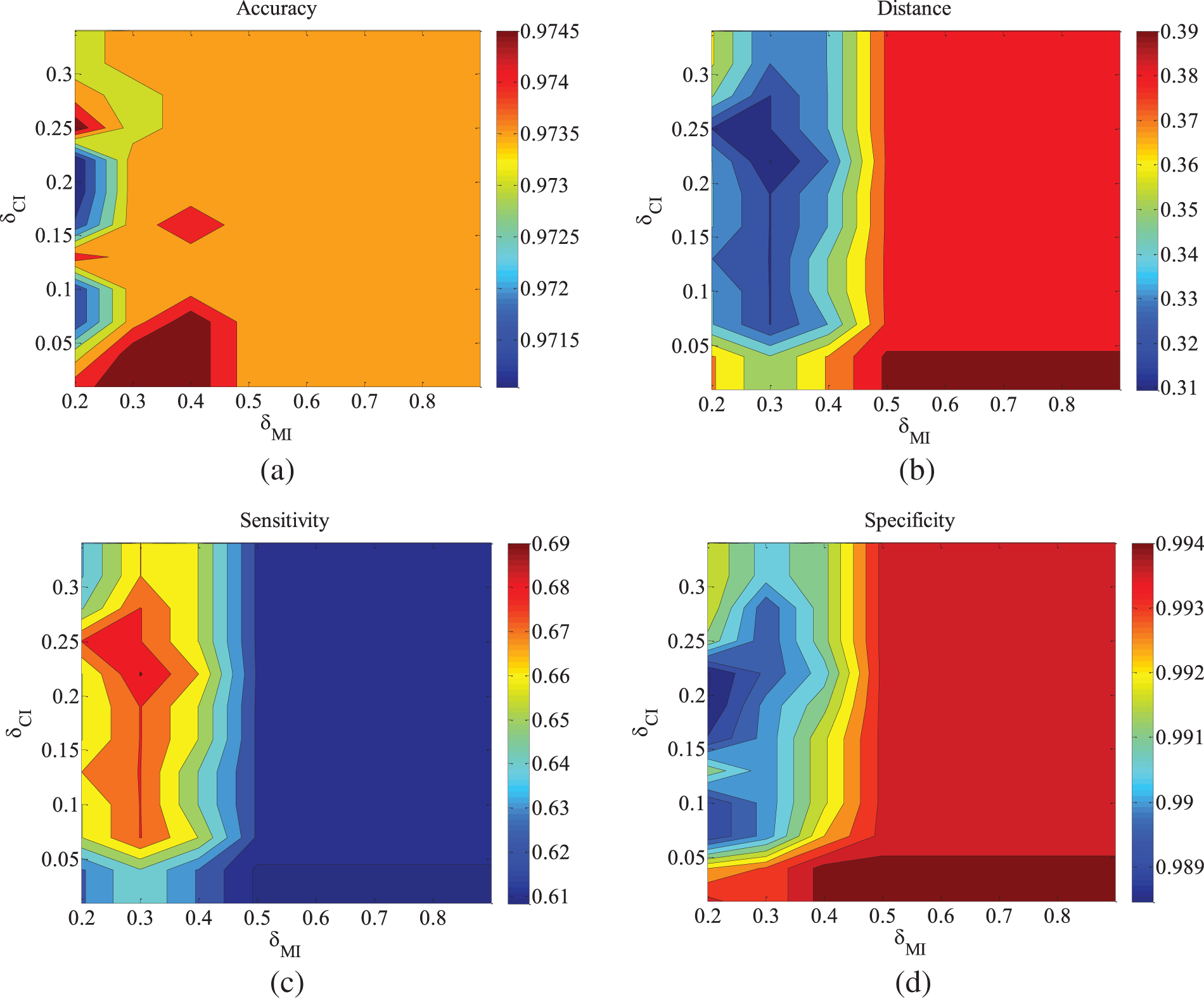
Figure 5: CHILD3-500 data set parameter changes. (a) Accuracy; (b) Euclid Distance; (c) True positive rate; (d) False positive rate

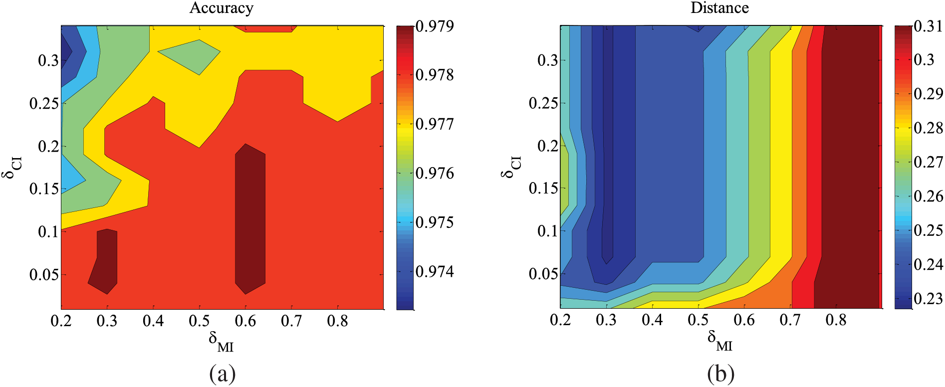
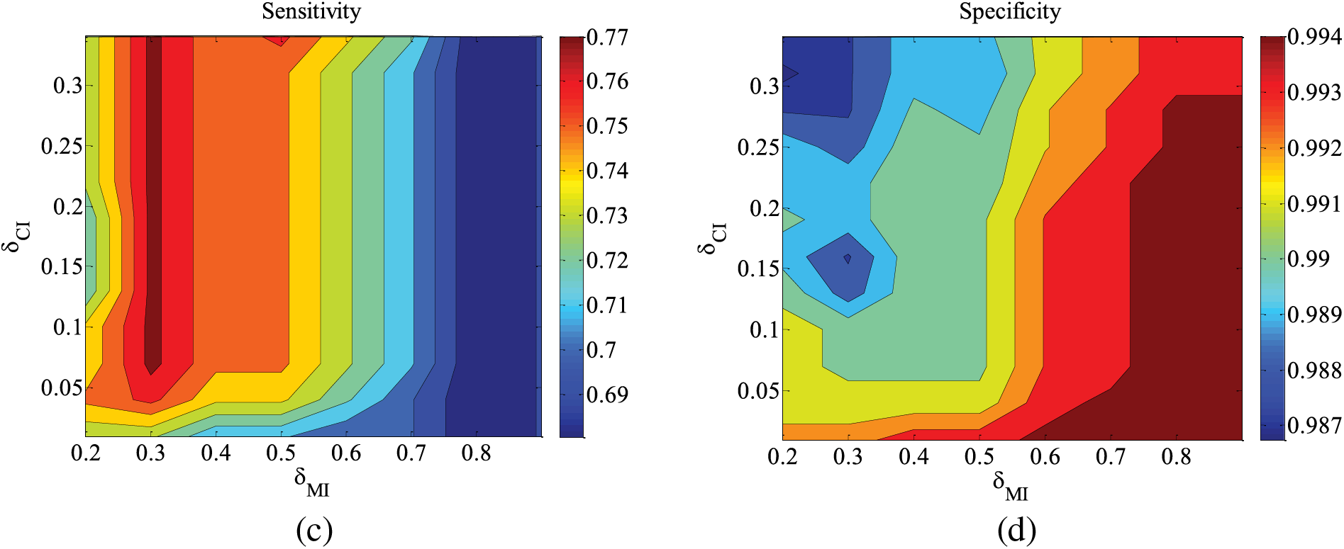
Figure 6: CHILD3-1000 data set parameter changes. (a) Accuracy; (b) Euclid Distance; (c) True positive rate; (d) False positive rate

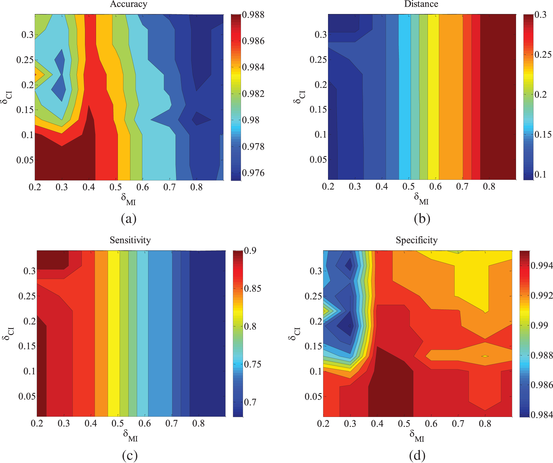
Figure 7: CHILD3-5000 data set parameter changes. (a) Accuracy; (b) Euclid Distance; (c) True positive rate; (d) False positive rate

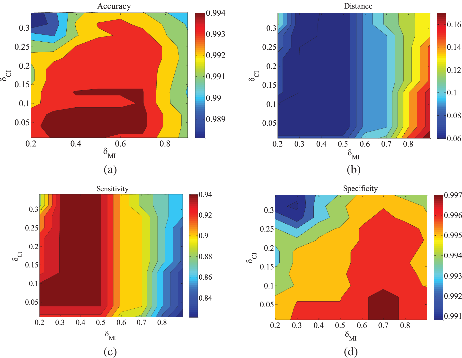
Figure 8: CHILD5-5000 dataset parameter changes. (a) Accuracy; (b) Euclid Distance; (c) True positive rate; (d) False positive rate

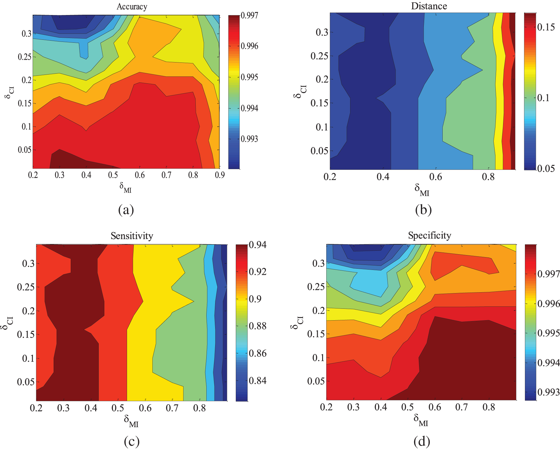
Figure 9: CHILD10-5000 dataset parameter changes. (a) Accuracy; (b) Euclid Distance; (c) True positive rate; (d) False positive rate

Figs. 2–4 are the experimental results of the ALARM network under different data sets. According to the definition of the evaluation metrics, a higher Accuracy value indicates that the algorithm’s learned undirected graph is closer to the true graph. From Figs. 2–4, it can be observed that as δMI increases while keeping other parameters fixed, the Accuracy values of the algorithm decrease, and a similar trend is seen with parameter δCI. Regarding the Euclidean Distance, which reflects the similarity between the learned undirected graph and the standard model, the smallest Euclidean Distance values are achieved when δMI is between 0.2 and 0.5, with the trend showing an increase as δMI increases.

For the metrics of true positive rate and false positive rate, they respectively reflect the proportions of correct edges and incorrect edges among total edges. Across different datasets of the ALARM network, both metrics show an increasing trend in error rates as δMI increases. In the initial stage of the algorithm, the value of δMI determines the proportion of added edges in the empty graph. Therefore, it is desirable to add a higher number of effective connecting edges in the initial stage to include a greater number of correct edges. However, as the algorithm progresses into its second stage, the introduction of parameter δCI validates the initial structure and eliminates false positive connections. To ensure accuracy, the value of δCI in this stage should not be too large.

In order to find a reasonable parameter setting for generalization, the algorithm’s testing dataset is further expanded. Subsequent observations will focus on the situations in other networks.

Figs. 5–9 illustrate the trends of parameter changes across different datasets. Similar to the ALARM network, the trends of parameter changes in terms of accuracy and Euclidean Distance are observed. Analyzing the true positive rate and false positive rate, these metrics reflect the proportions of correct edges and incorrect edges among all relevant statistical results. Therefore, a higher true positive rate indicates a greater number of correct edges obtained, while a lower false positive rate indicates fewer incorrect edges. Based on several sets of experimental results, it can be observed that when the value of δCI is fixed, the true positive rate and false positive rate achieve optimal values when δMI is between 0.2 and 0.5, and deteriorate as δMI increases beyond this range. Conversely, fixing the value of δMI has a smaller impact on δCI. Therefore, based on this analysis, to balance the relationships between these evaluation metrics, we aim to choose intermediate values for the parameters. Specifically, the value of δMI should be within the range of 0.2 to 0.5, and the value of δCI should be within the range of 0.05 to 0.1. For the sake of convenience in subsequent simulation experiments, we will set the parameters to their final values as δMI is 0.35 and δCI is 0.075.

4.2 Algorithm Performance Results

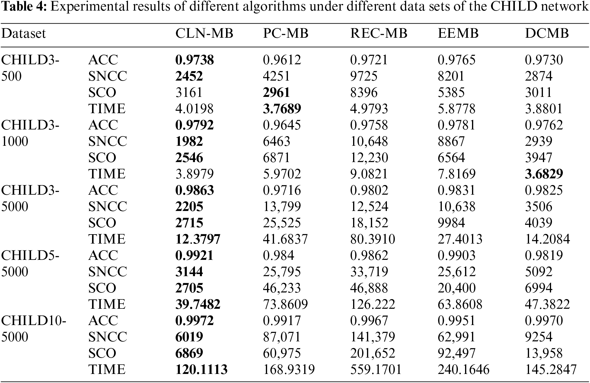
In order to verify the effectiveness of the algorithm, the algorithm in this paper is compared with other three algorithms, PC [20], REC [24], EEMB [27], DCMB [26], and the algorithm only compares the part of the construction of the undirected independent graph. The algorithm in this paper is based on the Markov blanket algorithm of locally constrained neighborhoods abbreviated as CNL-MB. The comparative experiment also uses the standard data sets ALARM, CHILD3, CHILD5 and CHILD10 from 5 different databases. ALARM and CHILD3 database select 3 different scale data sets of 500, 1000, 5000. CHILD5 and CHILD10 select 5000 data sets. The evaluation index selects the algorithm accuracy (ACC), the sum of the number of CI test calls (SNCC), the sum of CI test order for evaluation (SCO) and running time (TIME). The experimental results are shown in the Tables 3 and 4.

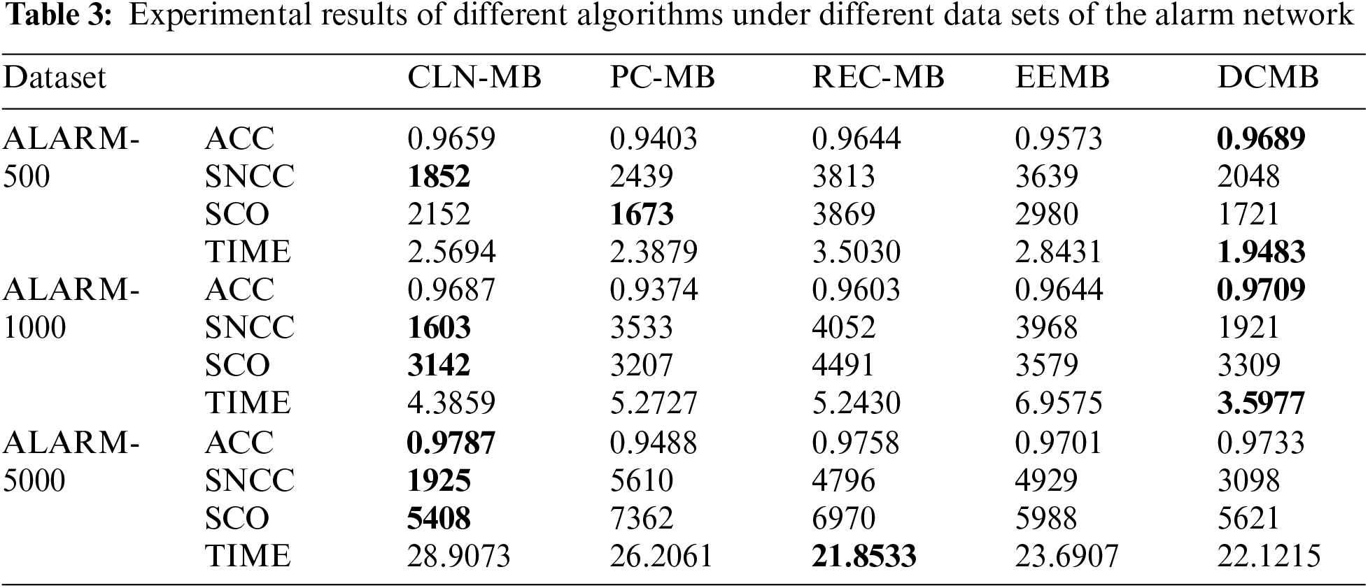
As can be seen from Table 3, we indicated the optimal value of each result in bold font. Using the same ALARM network for undirected independent graph restoration process, the algorithm in this paper not only has advantages in accuracy, but also can use fewer CI tests and fewer low-level CI tests. When using 500 sets of data, DCMB has a higher accuracy rate. This is because DCMB uses “and” and “or” rules to correct errors. So that more detailed information can be obtained, and it can be relatively accurate in the later use of CI judgments. But the opposite effect is that the smaller the subset, the more CI judgments will be used later. As the scale of the test data set continues to increase, the algorithm in this paper shows greater advantages. In 1000 and 5000 sets of data, because more local constraint node information is obtained, it is guaranteed to use fewer and lower-level CI tests in the later stage. In terms of running time, since the dataset size is not large, there is not much difference between the algorithms.

For the CHILD3, CHILD5 and CHILD10 dataset in Table 4, the increase in the number of nodes and edges has increased the difficulty of obtaining results, but the algorithm CLN-MB in this paper can still achieve higher accuracy. Compared with the other three algorithms, it still leads other algorithms CI test. This is attributed to the algorithm’s utilization of a constraint radius during initialization to obtain superior local information, enabling more efficient conditional independence testing in later stages.

In contrast to the PC-MB algorithm, because the PC-MB algorithm uses randomly selected nodes for CI testing during initialization. Therefore, the algorithm in this paper can accurately and quickly find and connect nodes with high correlation under the guidance of Markov blanket. This also prevents the algorithm from using high-level CI tests, further saving computational costs. Compared with the EEMB algorithm, the advantage of this paper is that the EEMB algorithm can only update the Markov blanket once, which makes it easy to lose key nodes, so the accuracy rate obtained is low. The algorithm in this paper makes the Markov blanket set more perfect through initialization and second update, and the low-order CI test also ensures the efficiency of the algorithm. The DCMB algorithm has a certain advantage in computational efficiency, but as the dataset size increases, our algorithm demonstrates a greater advantage in the number of CI test calls. From the experimental data, it is evident that compared to other algorithms, the algorithm presented in this chapter achieves higher accuracy with fewer conditional independence tests and using lower-order tests. This capability primarily stems from the adjustment of distance parameters to reduce computational complexity after the initialization phase of the algorithm. In the case of the ALARM network, where the network size contains relatively less local information compared to other datasets in this paper, the advantage of this approach is less pronounced in terms of computational results. However, the algorithm’s ability to achieve high accuracy with reduced testing frequency and lower-order tests showcases its efficiency and effectiveness across different datasets and network complexities.

5  Conclusions

We proposed a Markov blanket discovery algorithm based on local neighborhood space, which restricts the spatial range of the initial set by constraining the local neighborhood space of nodes. At the same time, the Markov blanket discovery algorithm is used to complete the constraint on the search space, and the two effectively reduce the frequency of use of the CI test. The establishment of local constraint factors greatly reduces the use of high-order CI test through experimental simulation, the values of the two parameters proposed by the algorithm are first determined. Under the same network model, through different datasets compared with other algorithms. The algorithm in this paper has a higher accuracy rate and uses fewer CI tests and lower-level CI tests. In future work, how to achieve the accuracy of the algorithm under a small data set can be used as a research content.

Acknowledgement: The authors wish to acknowledge Jingguo Dai and Yani Cui for their help in interpreting the significance of the methodology of this study.

Funding Statement: This work is supported by the National Natural Science Foundation of China (62262016, 61961160706, 62231010), 14th Five-Year Plan Civil Aerospace Technology Preliminary Research Project (D040405), the National Key Laboratory Foundation 2022-JCJQ-LB-006 (Grant No. 6142411212201).

Author Contributions: The authors confirm contribution to the paper as follows: study conception and design: Kun Liu, Peiran Li; methodology: Yu Zhang, Xianyu Wang; validation: Kun Liu, Ming Li, and Cong Li; formal analysis: Kun Liu, Peiran Li, Yu Zhang, Jia Ren; investigation: Ming Li, Cong Li; resources: Xianyu Wang; data curation: Kun Liu, Peiran Li and Ming Li; draft manuscript preparation: Kun Liu, Peiran Li; writing—review and editing: Kun Liu, Yu Zhang; supervision: Yu Zhang, Jia Ren; project administration: Jia Ren, Xianyu Wang, and Yu Zhang; funding acquisition: Jia Ren and Cong Li. All authors reviewed the results and approved the final version of the manuscript.

Availability of Data and Materials: Data available on request from the authors. The data that support the findings of this study are available from the corresponding author, Yu Zhang, upon reasonable request.

Ethics Approval: Not applicable.

Conflicts of Interest: The authors declare that they have no conflicts of interest to report regarding the present study.

References

1. M. Scanagatta, A. Salmerón, and F. Stella, “A survey on Bayesian network structure learning from data,” Prog. Artif. Intell., vol. 8, no. 4, pp. 425–439, 2019. doi: 10.1007/s13748-019-00194-y. [Google Scholar] [CrossRef]

2. W. Yang, M. S. Reis, V. Borodin, M. Juge, and A. Roussy, “An interpretable unsupervised Bayesian network model for fault detection and diagnosis,” Control Eng. Pract., vol. 127, no. 3, pp. 105304, 2022. doi: 10.1016/j.conengprac.2022.105304. [Google Scholar] [CrossRef]

3. Q. Xia, Y. Li, D. Zhang, and Y. Wang, “System reliability analysis method based on TS FTA and HE-BN,” Comput. Model. Eng. Sci., vol. 138, no. 2, pp. 1769–1794, 2024. doi: 10.32604/cmes.2023.030724. [Google Scholar] [CrossRef]

4. M. Yazdi and S. Kabir, “A fuzzy Bayesian network approach for risk analysis in process industries,” Process Saf. Environ. Prot., vol. 111, pp. 507–519, 2017. doi: 10.1016/j.psep.2017.08.015. [Google Scholar] [CrossRef]

5. Y. Ruan et al., “Noninherited factors in fetal congenital heart diseases based on Bayesian network: A large multicenter study,” Congenit. Heart Dis., vol. 16, no. 6, pp. 529–549, 2021. doi: 10.32604/CHD.2021.015862. [Google Scholar] [CrossRef]

6. T. Afrin and N. Yodo, “A probabilistic estimation of traffic congestion using Bayesian network,” Measurement, vol. 174, no. 2, pp. 109051, 2021. doi: 10.1016/j.measurement.2021.109051. [Google Scholar] [CrossRef]

7. B. G. Marcot and T. D. Penman, “Advances in Bayesian network modelling: Integration of modelling technologies,” Environ. Model. Softw., vol. 111, no. 1, pp. 386–393, 2019. doi: 10.1016/j.envsoft.2018.09.016. [Google Scholar] [CrossRef]

8. A. L. Madsen, F. Jensen, A. Salmerón, H. Langseth, and T. D. Nielsen, “A parallel algorithm for Bayesian network structure learning from large data sets,” Knowl.-Based Syst., vol. 117, no. 3, pp. 46–55, 2017. doi: 10.1016/j.knosys.2016.07.031. [Google Scholar] [CrossRef]

9. M. Lasserre, R. Lebrun, and P. H. Wuillemin, “Constraint-based learning for non-parametric continuous bayesian networks,” Ann. Math. Artif. Intell., vol. 89, no. 10, pp. 1035–1052, 2021. doi: 10.1007/s10472-021-09754-2. [Google Scholar] [CrossRef]

10. T. Gao, K. Fadnis, and M. Campbell, “Local-to-global Bayesian network structure learning,” in Int. Conf. Mach. Learn., Sydney, Australia, 2017, pp. 1193–1202. [Google Scholar]

11. M. Scutari, “Dirichlet Bayesian network scores and the maximum relative entropy principle,” Behaviormetrika, vol. 45, no. 2, pp. 337–362, 2018. doi: 10.1007/s41237-018-0048-x. [Google Scholar] [CrossRef]

12. C. He, X. Gao, and K. Wan, “MMOS+ ordering search method for bayesian network structure learning and its application,” Chin. J. Electron., vol. 29, no. 1, pp. 147–153, 2020. doi: 10.1049/cje.2019.11.004. [Google Scholar] [CrossRef]

13. H. Li and H. Guo, “A hybrid structure learning algorithm for Bayesian network using experts’ knowledge,” Entropy, vol. 20, no. 8, pp. 620, 2018. doi: 10.3390/e20080620. [Google Scholar] [PubMed] [CrossRef]

14. B. Sun, Y. Zhou, J. Wang, and W. Zhang, “A new PC-PSO algorithm for Bayesian network structure learning with structure priors,” Expert. Syst. Appl., vol. 184, no. 1, pp. 115237, 2021. doi: 10.1016/j.eswa.2021.115237. [Google Scholar] [CrossRef]

15. J. Liu and Z. Tian, “Verification of three-phase dependency analysis Bayesian network learning method for maize carotenoid gene mining,” Biomed Res. Int., vol. 2017, no. 1, pp. 1–10, 2017. doi: 10.1155/2024/6640796. [Google Scholar] [CrossRef]

16. V. R. Tabar, F. Eskandari, S. Salimi, and H. Zareifard, “Finding a set of candidate parents using dependency criterion for the K2 algorithm,” Pattern Recognit. Lett., vol. 111, no. 3, pp. 23–29, 2018. doi: 10.1016/j.patrec.2018.04.019. [Google Scholar] [CrossRef]

17. D. Heckerman, D. Geiger, and D. M. Chickering, “Learning Bayesian networks: The combination of knowledge and statistical data,” Mach. Learn., vol. 20, no. 3, pp. 197–243, 1995. doi: 10.1007/BF00994016. [Google Scholar] [CrossRef]

18. C. P. de Campos, M. Scanagatta, G. Corani, and M. Zaffalon, “Entropy-based pruning for learning Bayesian networks using BIC,” Artif. Intell., vol. 260, no. 4, pp. 42–50, 2018. doi: 10.1016/j.artint.2018.04.002. [Google Scholar] [CrossRef]

19. P. Spirtes, C. N. Glymour, R. Scheines, and D. Heckerman, Causation, Prediction, and Search. Cambridge, MA, USA: MIT Press, 2000. [Google Scholar]

20. P. Spirtes and C. Glymour, “An algorithm for fast recovery of sparse causal graphs,” Soc. Sci. Comput. Rev., vol. 9, no. 1, pp. 62–72, 1991. doi: 10.1177/089443939100900106. [Google Scholar] [CrossRef]

21. A. Cano, M. Gómez-Olmedo, and S. Moral, “A score based ranking of the edges for the PC algorithm,” in Proc. Fourth Euro. Workshop Probabilistic Graphic. Model., Cuenca, Spain, 2008, pp. 41–48. [Google Scholar]

22. D. Colombo and M. H. Maathuis, “Order-independent constraint-based causal structure learning,” J. Mach. Learn. Res., vol. 15, no. 1, pp. 3741–3782, 2014. [Google Scholar]

23. J. Cheng, R. Greiner, J. Kelly, D. Bell, and W. Liu, “Learning Bayesian networks from data: An information-theory based approach,” Artif. Intell., vol. 137, no. 1–2, pp. 43–90, 2002. doi: 10.1016/S0004-3702(02)00191-1. [Google Scholar] [CrossRef]

24. X. Xie and Z. Geng, “A recursive method for structural learning of directed acyclic graphs,” The J. Mach. Learn. Res., vol. 9, pp. 459–483, 2008. [Google Scholar]

25. I. Tsamardinos, L. E. Brown, and C. F. Aliferis, “The max-min hill-climbing Bayesian network structure learning algorithm,” Mach. Learn., vol. 65, no. 1, pp. 31–78, 2006. doi: 10.1007/s10994-006-6889-7. [Google Scholar] [CrossRef]

26. X. Guo, K. Yu, L. Liu, F. Cao, and J. Li, “Causal feature selection with dual correction,” IEEE Trans. Neural Netw. Learn. Syst., vol. 35, no. 1, pp. 938–951, 2022. doi: 10.1109/TNNLS.2022.3178075. [Google Scholar] [PubMed] [CrossRef]

27. H. Wang, Z. Ling, K. Yu, and X. Wu, “Towards efficient and effective discovery of Markov blankets for feature selection,” Inf. Sci., vol. 509, pp. 227–242, 2020. doi: 10.1016/j.ins.2019.09.010. [Google Scholar] [CrossRef]

28. X. Guo, K. Yu, F. Cao, P. Li, and H. Wang, “Error-aware Markov blanket learning for causal feature selection,” Inf. Sci., vol. 589, no. 4, pp. 849–877, 2022. doi: 10.1016/j.ins.2021.12.118. [Google Scholar] [CrossRef]

29. D. Husmeier, “Sensitivity and specificity of inferring genetic regulatory interactions from microarray experiments with dynamic Bayesian networks,” Bioinformatics, vol. 19, no. 17, pp. 2271–2282, 2003. doi: 10.1093/bioinformatics/btg313. [Google Scholar] [PubMed] [CrossRef]