Adaptive Graph Convolutional Adjacency Matrix Network for Video Summarization

1  Introduction

With the booming development of social networks, a large number of user-created videos have emerged on major online platforms. These videos are of various forms and lengths, mainly narrative short films and life records. This not only enriches people’s lives, but also allows users to record their lives by making videos. However, most users prefer to browse specific scenes or events in the videos rather than the complete videos content [1]. The massive amount of video data poses a huge challenge for retrieval, storage and browsing [2]. Therefore, video summarization techniques have become a popular research topic.

Video summarization techniques aim to generate summaries by extracting key frames or key shots in a video to present the video in a condensed form while ensuring that the most informative segment are retained [3]. Based on the type of summaries generated, video summarization can be categorized into two main types: static video summarization and dynamic video summarization [4]. Static video summarization form a collection of summaries by selecting the most representative key frames from the video. The summaries are presented in the form of images, similar to a slide presentation, which may not fully capture the main content of video. In contrast, dynamic video summarization involves selecting key shots comprising images, audio and text data, enabling a more comprehensive portrayal of the video content. For instance, consider Fig. 1, depicting a crime surveillance video from UCF_Crimes capturing a criminal in the act of theft. In such scenarios, the objective of video summarization is to identify the segments with high relevance scores, as illustrated in the figure, and generate summaries without necessitating a complete viewing of the entire video.

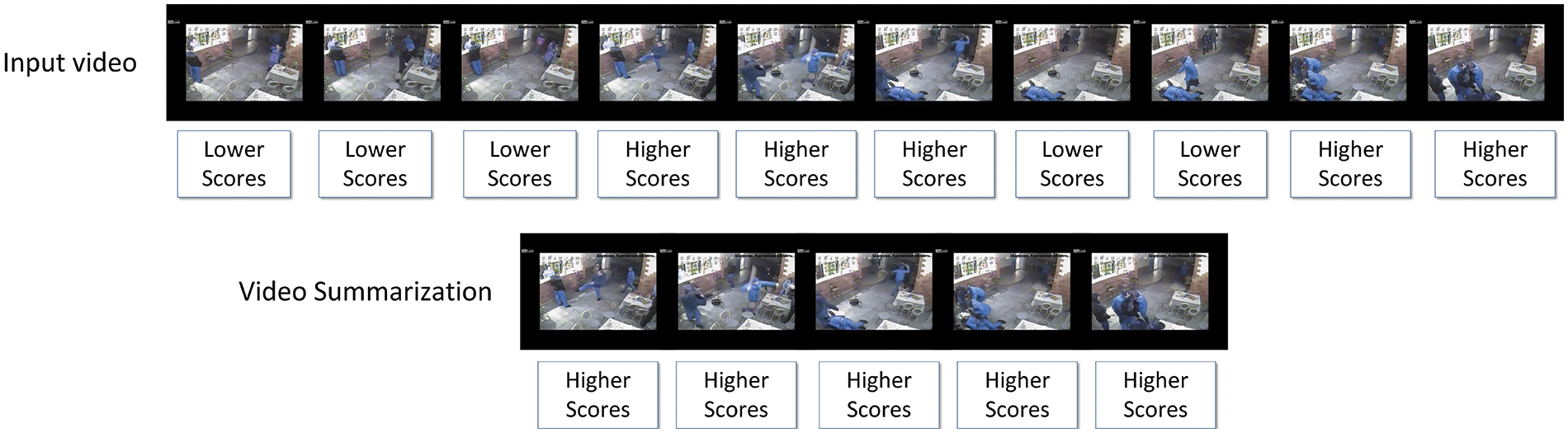
Figure 1: Video summarization overview

1.1 Motivation and Overview

In recent years, deep learning techniques have seen widespread applization in video processing tasks [5–8], notably advancing the field of video summarization [9]. Video summarization methods are categorized primarily based on their use of labels into three main groups: supervised video summarization, unsupervised video summarization and weakly supervised video summarization [2]. Supervised video summarization methods rely on extensive labeled video data with detailed score annotations. Although these supervised methods are capable of generating high-quality summaries using detailed labelling information, their annotations are costly. In contrast, unsupervised video summarization methods do not rely on labeled data during training, instead employing adversarial training or reconstruction techniques. Compared to supervised video summarization methods, the generated summaries may not be as accurate as supervised methods due to the lack of direct supervisory information. Weakly supervised video summarization methods, situated between supervised and unsupervised approaches, typically utilize only video-level labels, such as video title or categories, without detailed frame or timing labels. While the quality of summaries produced by weakly supervised methods may not match that of supervised approaches, they still benefit from some level of supervisory signals compared to unsupervised methods. In this paper, we adopt a supervised video summarization approach. Zhao et al. [10] and Hu et al. [11] employed recurrent neural networks (RNNs) to capture the temporal dependencies within video frame sequences, generating concise and representative video summaries. Lin et al. [12] integrated the attention mechanism with a bidirectional long short-term memory (BiLSTM) network, enabling the model to prioritize important segments while disregarding irrelevant information during sequence processing. Despite the prone to issues like gradient vanishing and explosion inherent to RNNs, the above methods still suffer from the problems of gradient vanishing and gradient explosion due to the inherent defects of RNNs. The introduction of Graph Neural Networks (GNN) allows the model to better simulate global dependencies. Within a graph-based framework, video features are treated as nodes of the graph, with inter-node similarities serving as edge weights. Initially, Wu et al. [13] utilised Graph Convolutional Networks (GCNs) for multi-video summarization, effectively capturing global dependencies across multiple videos. Li et al. [14] and Zhong et al. [15] introduced Graph Attention Networks (GATs) to mitigate redundancy among key frames in video summarization. However, prior GNN models featured fixed graph structures, where node features are updated to higher-level representations with each convolution operation. However, these methods have a limitation: the adjacency matrix remains static and fails to reflect new changes in graph structure and attributes. To adress this, we propose a novel approach that leverages attention to dynamically adjust adjacency matrix weights. Initially, we segment shots and extract frame features, then compute representative features for each shot. Treating shot features as graph nodes, we construct a graph using shot features similarity as edges weights. Subsequently, we introduce an attention mechanism to dynamically assign adjacency matrix weights, better capturing dynamic node dependencies. To enhance summarization quality, we fuse the temporal features extracted by BiLSTM with the structural features extracted by graph convolutional networks through feature fusion. We conduct extensive experiments on two benchmark datasets, TVSum and SumMe, achieving F1-score of 60.8% and 53.2%, respectively. Results demonstrate our method’s superiority over current state-of-the-art video summarization techniques, validating its effectiveness in capturing dynamic node dependencies.

1.2 Contribution

The contribution of the method proposed in this paper is as follows:

1)   In this paper, we present an adaptive graph convolutional adjacency matrix network for video summarization, addressing the issue of fixed neighbor aggregation in graph neural network-based methods.

2)   Leveraging BiLSTM for temporal feature extraction and TAMGCN for dynamic structural feature capture, our proposed TAMGCN effectively mitigates interference arising from shot distances.

3)   To achieve a comprehensive feature representation, we integrate temporal features from BiLSTM with structural features from graph convolutional networks.

4)   Extensive experiments on TVSum and SumMe datasets demonstrate the superiority of our approach over current state-of-the-art video summarization methods.

1.3 Organization

The rest of this article is organized as follows. Related work is reviewed in Section 1. The details of the proposed method are described in Section 2. Experimental results and analysis are presented in Section 3. The conclusion is drawn in Section 4.

2  Related works

2.1 Video Summarization

Presently, researchers primarily employ deep learning methods for video summarization techniques [4,8]. Video summarization approaches are typically categorized as supervised, unsupervised and weakly supervised methods [1] based on the use of labels. Supervised methods rely on manually labeled importance scores to guide summaries generation. To address long-term dependencies, Zhao et al. [10] introduced the Tensor Trained Hierarchical Recurrent Neural Network (TTH-RNN), which mitigates the issue of large features mapping to hidden matrix through tensor training of the embedding layer. They also designed a hierarchical RNN structure to explore long term dependencies between video frames. Liu et al. [16] proposed the Hierarchical Multi-Headed Attention Network (H-MAN), leveraging the multi-head attention mechanism to enhance model performance. Liang et al. [17] proposed an approach employing self-attention mechanism and fully convolutional sequential network to capture both global and local temporal dependencies among video frames. They further designed a convolutional attention-generating adversarial network for implementing unsupervised video summarization. Hu et al. [18] introduced a video summarization method based on generative adversarial network (GANs), where discriminator not only assesses the the video’s integrity, but also evaluates the importance of candidate key frames, thus significantly impacting the final summarization outcome. Regarding weakly-supervised video summarization methods, researchers commonly utilize relatively weak labels such as video titles or outlines for training the summaries process. Panda et al. [19] approached video summarization as a weakly-supervised learning task, proposing a flexible and deep 3DCNN architecture that leverages video-level annotations to learn key frames without relying on manually generated training data. Furthermore, Ho et al. [20] introduced a novel deep neural network architecture aimed at describing and distinguishing important spatio-temporal information in videos with different viewpoints. Implemented in a semi-supervised setting, the model combines fully labeled third-person videos, unlabeled first-person videos, and a small amount of labeled first-person videos for training.

2.2 Graph Neural Network

In recent years, graph neural networks have gained widespread adoption in computer vision. Among these, graph convolutional networks (GCNs) are utilized to acquire high-level feature representations of nodes by aggregating features from each graph node and its neighbors. Typically, GCNs comprise multiple layers. Despite significant progress in various domains, the static nature of the neighborhood matrix used in GCNs somewhat constrains the model’s effectiveness. To address this constraint, Graph Attention Networks (GATs) employ attention mechanism to automatically learn and optimise connectivity relationships between nodes. Zhao et al. [21] designed a sequence graph architecture that hierarchically captures intra-shot temporal dependencies and inter-shot pairwise dependencies through LSTM and GCN, effectively mitigating interference arising from shot positions. Zhong et al. [15] proposed a graph-based Attention Network (GAT) model for bidirectional long-term and short-term memory (Bi-LSTM), employing a Contextual Feature Based Transformation (CFT) mechanism to convert visual features of an image to higher level features. Zhu et al. [22] leveraged object-level and relational-level information to capture spatio-temporal dependencies. Their approach involves constructing a spatial graph of the target object post target detection, followed by constructing a temporal map using an aggregated representation of the spatial map.

3  Attention Adaptive Adjacency Matrix GCN

In this paper, we introduce an innovative adaptive graph convolutional adjacency matrix network aimed at addressing the issue of aggregating neighbors with fixed weights once the adjacency matrix is determined in graph convolutional neural networks. Fig. 2 shows a brief framework of our proposed model, comprising three crucial components: The initial stage involves segmenting the input video into shots and extracting image features from each video frame using a convolutional neural network. Subsequently, in the second part, representative frames are selected, shot data is condensed, and the adjacency matrix is constructed. In the third part, TAMGCN is employed to compute structural features. Finally, feature fusion is utilized to calculate the score for each shot. Additionally, we have designed a sparsity rule to train the network, promoting the selection of diverse abstracts. The following sections provide more details on our proposed method.

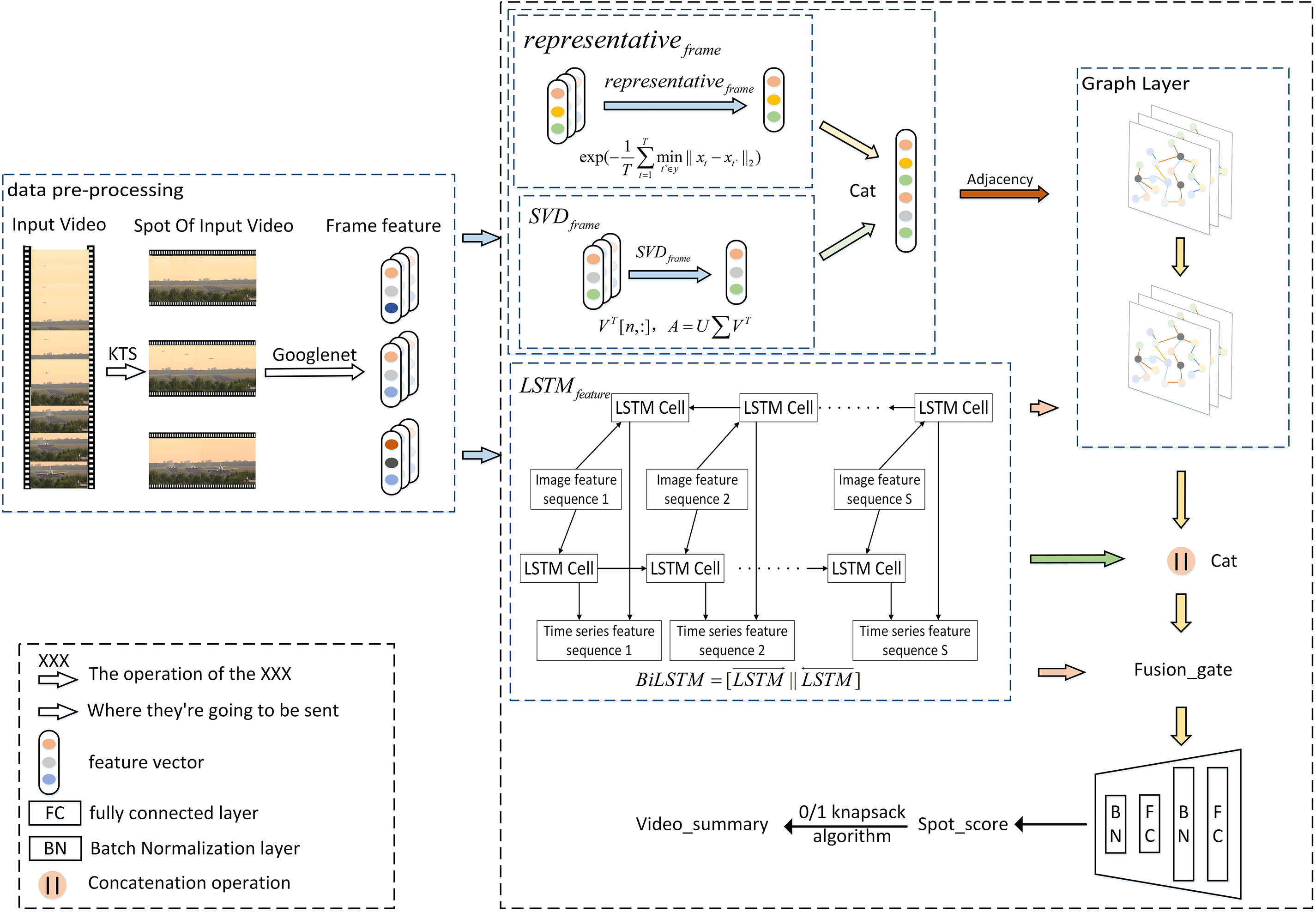
Figure 2: The overall framework of model (TAMGCN)

3.1 Preprocessing

The sequence of input video frames is defined as X={xn}n=1N, X, where N represents the number of video frames contained in each video, w,h,3 represents the width, height, and the number of channels of each picture frame, and xn represents the n video frame. The kernel temporal segmentation (KTS) algorithm [23] obtains shot sequence S={sm}m=1M,sm∈Rw×h×3×Tm, where M means that a video is divided into M shots, and sm means there are Tm frames in the m shots and N=∑m=1MTm.

Pre-training model GoogleNet [21] was used to extract image feature Sfeature={sm′}m=1M,sm′∈RF×Tm, sm′ means that the m shot has Tm frames, and F is the feature dimension of each frame. Local feature Sdata of each video is obtained by the bidirectional encoding of LSTM from Sfeature:

Sdata=BiLSTM(Sfeature)=[LSTM(Sfeature)→||LSTM(Sfeature)←](1)

where BiLSTM(⋅) represents a bidirectional LSTM, which is composed of two LSTM splices in different directions. The output of BiLSTM(⋅) is the last hidden layer ht∈RF×Tm because the previous ht frame encodes the timing information of forwarding and backwards in the current shot. Here, the final frame∈RF of each shot output ht is taken and stacked as the local feature Sdata∈RF×M of the whole video.

3.2 Construction of Adjacency Matrix

To utilize graph neural networks for video summarization, the video must initially be represented as a graph structure, comprising vertices and edges. In the video summarization task, the shot features of a video are designated as nodes of a graph. According to the thesis, the similarity between shots features is defined as the weights of the top edges of the graph. The shots features are defined as follows:

Spotfeature=[representativeframe||SVDframe](2)

In our approach, the node feature Spotfeature∈R2F×M is spliced from representative features and singular value features. Inspired by representative rewards in reinforcement learning, we introduce the representative feature representativeframe∈RF×M. Specifically, there is a large amount of redundancy due to the fact that frames in a shot are usually similar. In order to extract the most representative frames, we determine the most representative frames in each shot through representativeness computation and use their features as shot features. To select the most representative frames, we calculated the 2-parameter number between frames and other frames in each shot and selected the frame with the lowest average parameter number as the representative frame for that shot. This process helps to reduce redundant information, allowing the shot features to effectively reflect the video content.

The weights of edges on a graph are usually computed from the similarity between nodes. Edges on the graph do not only indicate the connectivity between nodes, but may also contain some additional information about the degree of similarity or association between nodes. In order to more accurately reflect the relationship between nodes, we can measure the weights of edges by similarity calculation. This approach helps to capture the interrelationships between nodes more comprehensively in the graph structure and improves the performance of the video summarization model.

representativeframe=representative(Sfeature)=exp⁡(−1Tm∑t=1Tmmint′∈y||xt−xt||2)(3)

Compared with QR decomposition, which can only decompose matrix in a square matrix, singular value (SVD) decomposition algorithm as shown in Fig. 3 is a matrix decomposition algorithm that can decompose matrix at any scale, where U is the left singular matrix, which compresses the number of rows, VT is the right singular matrix, which compresses the number of columns, ∑(⋅) is the singular value, And the first n singular values in singular value ∑(⋅) occupy most of the sum of singular values.

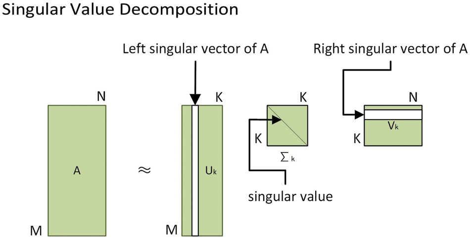
Figure 3: SVD decomposition diagram

Usually, the first n column of left singular matrix U is taken as the main feature of the matrix, but this method is not friendly to the shots with the variable frame number. For different shots, different frames result in different numbers of data in the first n columns of the left singular matrix, and data of indefinite length cannot be learned in the neural network. Therefore, the first n rows of the right singular matrix are taken as SVDframe of each shot in this paper:

A=u∑VT(4)

∑=[σ10⋯00σ2⋯0⋮⋮⋱⋮00⋯0](5)

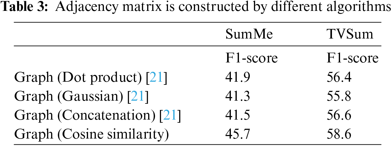
Video summarization does not inherently provide an explicit adjacency matrix, necessitating its generation. Once node features are acquired, the similarity between paired nodes is computed to establish the corresponding edges, thus determining the values of the adjacency matrix. Building upon the work of Zhao et al. [21], we explored four functions for edge weight calculation, and their expressions are as follows:

1)   Dot Product [14,21]

eij=f(xi,xj)=−ϕ(xi)Tφ(xj)(6)

2)   Gaussian [21]

eij=f(xi,xj)=exp⁡{−ϕ(xi)Tφ(xj)}(7)

3)   Concatenation [21]

eij=f(xi,xj)=WeT[ϕ(xi)||φ(xj)](8)

4)   Cosine similarity [23]

eij=f(xi,xj)=xiTxj||xi||2⋅||xj||2(9)

X is the feature of each node Spotfeature, and [⋅||⋅] is the connection operation. ϕ(⋅), φ(⋅) are linear transformations based on Wϕ,Wφ,Wϕ,Wφ,We are all learnable parameters. The adjacency matrix Aadj∈RM×M is constructed by the above method.

3.3 Attention Adaptive Adjacency Matrix

3.3.1 Graph Attention

As shown in Fig. 4, to overcome the effect of a fixed adjacency matrix on each layer of GCN, the attention mechanism is used in TAMGCN to ensure that the effect of the adjacency matrix on each layer is different. Inspired by GAT, the attention of each layer is calculated according to the input Sdata of the current layer. The attention of the current node is calculated as follows:

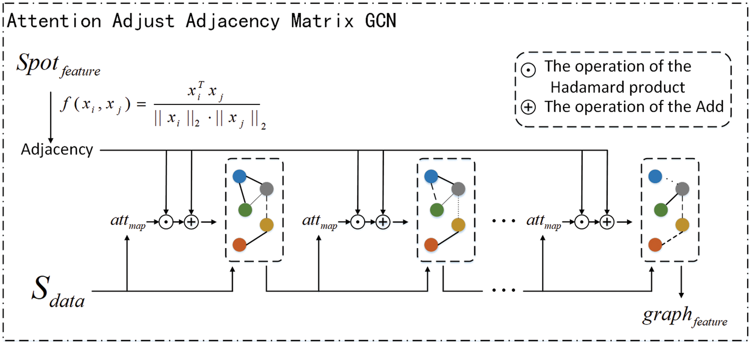
Figure 4: The model of attention adjust adjacency matrix GCN

eij=LeakeyReLU(α→[USdatai→||USdataj→])(10)

Sdata,i∈[1,M] represents the current node, Sdataj,j∈[1,M−1] represents the neighbour node, U∈RF×F′ is the weight matrix that can be learned, [⋅||⋅] means the join operatio, LeakyReLU(⋅) is quoted here as the activation function, and α→∈R2F′×1 is the attention distribution matrix that can be learned.

aij=Nj(eij)(11)

aij is attention weight, N(⋅)=exp⁡(⋅)/∑exp⁡(⋅) is the normalization operator. The final output of graph attention for the entire layer is attmap∈RM×M.

3.3.2 Attention Adaptive Adjacency Matrix

TAMGCN model f(Sdata,Aadj,attmap) learns the relationship between video shots, where Sdata represents the node features of the input video, attmap is the attention matrix calculated according to the input of Sdata the current layer, and Aadj is the adjacency matrix. Inspired by Kipf [23], TAMGCN of each layer is modelled based on GCN:

H(l+1)=σ(A~adjH(l)W(l))(12)

Here H(l)∈RM×F′ represents the output l=0,1,…,L−1, and H(0)=Sdata of layer l, and σ(⋅) is the activation function, e.g., ReLU(⋅)=max(0,⋅). Wl∈RFl×Fl+1 is the trainable weight matrix in each layer, and A~adj∈RM×M is the adjacency matrix after attention adjustment:

A~adj=Aadj⊙attmap+Aadj(13)

where attmap is the attention matrix generated according to H(l) of each layer, in this way, the influence of neighbour nodes on the current node can be dynamically adjusted according to different input data. TAMGCN output is graphfeature=H(L−1)∈RM×FL−1 and H(L−1) represent the graph output of the last layer, where FL−1 denotes the dimension of TAMGCN output of the last layer. To facilitate the migration of the model, we set dimension FL−1 to be the same as dimension F. In this design, additional parameter adjustments will not be made because the graph part is added to the model.

The algorithmic flow of the collective is as in Algorithm 1.

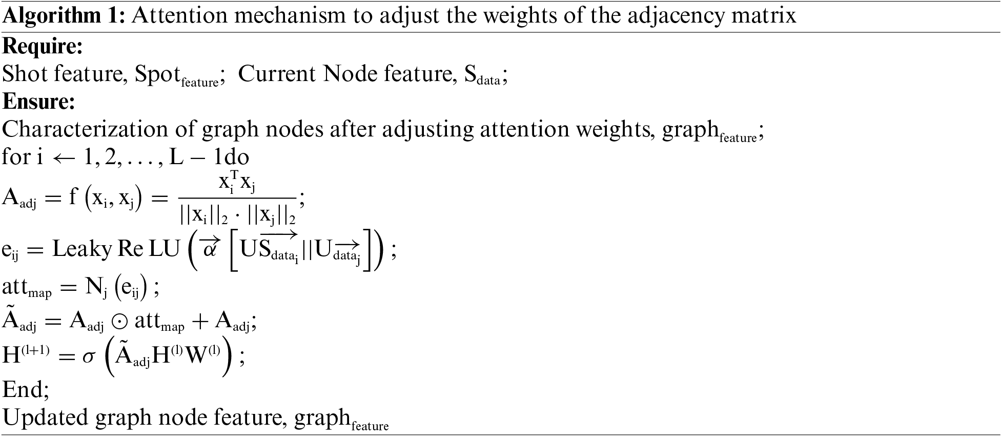
Traditional GAT is to adjust the weights of the initial adjacency matrix. And as the node features change, the weights of the original adjacency matrix are no longer adapted to the new node features, our Attention Adaptive Adjacency Matrix updates the adjacency matrix at each layer. The correlation between the adjacency matrix and the node features is improved in order to obtain a more accurate summaries.

3.3.3 Fusion Mechanism

To make graphfeature have timing feature Globalfeature of the video sequence, we use the fusion mechanism [24] to fuse feature graphfeature∈RF×M with timing feature Globalfeature. Here, local feature Sdata is sent to network BiLSTM(⋅), and the last layer of the hidden layer is taken as timing feature Globalfeature∈RF×M output:

Globalfeature=BiLSTM(Sdata)=[LSTM(Sdata)→||LSTM(Sdata)←](14)

These two features are first defined as R=[graphfeature||Globalfeature]∈R2F×M through connection operation, and then the whole fusion mechanism includes linear layer and activation layer:

R′=ReLU(WHR)∈RF×M(15)

Q=sigmoid(WQR)∈RF×M(16)

where WH∈R2F×F and WQ∈R2F×F are two learnable weight matrices, local feature Sdata∈RF×M and feature R′ are fused to maintain the original shot’s semantic information. Finally, the final shot fraction spotscore is obtained through multiple fully connected layers FC(⋅):

Spotscore=σ(FC(R′⊙Q+Sdata⊙(1−Q)))(17)

FC(⋅)=BN(Linear(⋅))(18)

σ(⋅) is the activation function of sigmoid(⋅), and Spotscore∈RM represents the non-negative score of each shot. The higher the score is, the more chance it has to be selected into the video summarization. After obtaining the shot score of each video, key shots were chosen according to the 0–1 knapsack algorithm to generate a video summarization.

3.4 Optimization of Model

The loss function is a function to measure the difference between the predicted value and the real value of the model. The smaller the loss function is, the more consistent the model and parameters are with the training samples. In this paper, the mean square error is used to calculate the loss of the model as follows. The obtained error represents the Euclidean distance between the predicted value and the actual value, where yreal represents the real score and yscore=spotscore represents the predicted score.

L(yreal,yscore)=1n∑i=1n(yreal−yscore)2(19)

In addition, considering that the goal of video summarization is to use a small number of shots to express the semantics of the whole video as much as possible, we tend to calculate that attmap in this model should be sparse, so we design a sparsity loss Lossatt to restrict the sparsity of attmap, which is defined as follows:

Lossatt=||attmap||1=∑iM∑jM||aij||1(20)

Our proposed model, TAMGCN, was performed on PyTorch. Specifically, with 300 training rounds, the dimensions of the hidden state are 512 and 1024 for both LSTM and graph aspects. To reduce the learning burden of the model and fix the adjacency matrix, feature extraction uses a pre-trained but not updated Google Net. Adam optimizer was used to optimize the whole architecture, and the initial learning rate was 0.01. The learning rate attenuated once every 30 rounds, and the decay rate gamma was 0.9.

4  Experimental Result and Analysis

4.1 Datasets and Evaluation Indicators

We conducted extensive experiments on two standard datasets, the SumMe dataset and the TVSum dataset. The SumMe dataset consists of 25 user-edited videos that range in length from about 1–6 min. Each of these videos is manually rated by multiple individuals. The TVSum dataset consists of 50 videos covering topics such as cooking, traveling, and sports. The length of the videos is longer than those in the SumMe dataset, about 2–10 min In order to compare with other state-of-the-art methods, this paper adopts the F1-score as an evaluation metric to measure the goodness of video summarization. The F1-score is a metric used to evaluate the performance of a binary classification model that combines the precision and recall of the model. When a category imbalance exists, the F1-score may tend to perform well on categories with more samples and poorly on categories with fewer samples.The F1-score only considers positive and negative examples in the model’s predictions, ignoring information beyond the true and true negative examples. In some cases, this may make the assessment of model performance less comprehensive. In this paper, we define the model-generated summarization as S and the manually annotated summarization as G. The correctness and recall rates are calculated as follows:

precision=overlaped duration of SandGduration of S(21)

recall=overlaped duration of SandGduration of G(22)

From the above formula, F1-score can be calculated to evaluate the generation of video summaries.

F1−score=2×precision×recall precision+recall×100\% (23)

4.2 Experimental Results and Discussion

In this paper, during the experiment, all data is divided into training and test sets, with 80% of the total data allocated to the training set and 20% to the test set. To avoid the influence of different videos on the experimental results, we implement a five-fold cross-validation [21]. Specifically,the video data is first randomly disrupted and divided into five parts using Python’s random library. The to the five results by five-fold cross-validation. In addition, according to the literature [25], for the SumMe dataset, the maximum of the 5 results is taken as the final result of the experiment. For the TVSum dataset, the final result of the experiment is taken as the average of the 5 results. In addition, according to the literature [25], for the SumMe dataset, the maximum of the 5 results is taken as the final result of the experiment. For the TVSum dataset, the final result of the experiment is taken as the average of the 5 results.

To validate the effectiveness of our proposed method, we conducted comparisons with current state-of-the-art video summarization techniques on two benchmark datasets, TVSum and SumMe. Among these, TTH-RNN [10] contains a tensor training embedding layer and a hierarchical LSTM. The tensor training embedding layer avoids the large number of features mapped to the hidden matrix due to high-dimensional video features, thus reducing training complexity by minimizing parameters. A-AVS and M-AVS [26] are an encoder-decoder video summarization model that introduces an attention mechanism. In the encoding stage, BiLSTM is utilized, while the decoding stage employs BiLSTM enhanced with attention mechanisms. A-AVS employs an additive attention mechanism for scoring, whereas M-AVS employs a punitive attention mechanism. PRLVS [25] is a progressive reinforcement learning video summarization network with unsupervised rewards, which emulates a ‘T’ type human thinking paradigm by removing most of the training parameters. ‘T’ type human thinking paradigm designed a horizontal strategy and a vertical strategy to alternately reason about the selection of key frames for choosing a selection action. These two strategies are hierarchically constructed to offer more comprehensive information than the planar strategy to ensure the completeness of the generated summaries. DSNet [27] is a Detection-Summarisation Network (DSNet) framework for supervised video summarization, comprising anchor-based and anchor-free methods. Anchor-based methods generate temporal interest proposals to identify and locate representative content in video sequence, while anchor-free methods eliminate predefined temporal proposals and directly predict importance scores. H-MAN [16] consists of a shot-level reconstruction model and a multiple-attention model, employing a two-stage hierarchical structure to generate diverse attention maps. SUM-GDA [14] is an efficient convolutional neural network architecture based on global change attention, which considers temporal relationships among video frames through a global view attention mechanism. RCLsup [28] is a framework that combines reinforcement and contrast learning for unsupervised video summarization, aiming to enhance feature representations and the model’s contextual modelling capabilities. Where contrast learning is used to facilitate discriminative row and informative shot-level feature learning. However, the proposed methos not only uses dynamic extraction of the structural features of the video, but also employs LSTM to capture the temporal features in the video. Besides, through experiments, we have set up the optimal feature fusion method to effectively integrate the timing features and the structural features.

The comparison results are presented in detail in Table 1. Our method exhibits significant improvements in F1-score on both datasets compared to TTH-RNN, A-AVS, and M-AVS methods. This may be attributed to the fact that the these methods fail to adequately capture the global structural features of the video, despite effectively leveraging the temporal information of the LSTM and the attention mechanism. In comparison to PRLVS, our proposed method achieves a 6.9% higher F1-score on the SumMe dataset, while on the TVSum dataset, it shows a slight inferiority to PRLVS, with a 2.2% decrease. This is because PRLVS is more suitable for modelling long videos, whereas our method excels with shorter ones. Against DSNet, our method holds a slight advantage on the SumMe dataset, whereas DSNet slightly outperforms our method on the TVSum dataset. This outcome partially confirms the effectiveness of our method. Compared to H-MAN, our method achieves a 3% higher F1-score on the SumMe dataset but trails slightly behind H-MAN on the TVSum dataset by 1.3%. This variance could be attributed to H-MAN’s hierarchical self-attention model, which is more adept at modelling longer videos, whereas layering short videos may have reduced the quality of the summaries. Compared to SUM-GDA, our method demonstrates strong performance across both datasets, as it not only incorporates temporal features but also comprehensively addresses structural features in videos. In comparison to RCLsup, our method exhibits a slight decrease of 0.8% on the SumMe dataset, and a larger discrepancy of 1.8% on the TVSum dataset. This variance may stem from RCLsup’s optimization of feature representation through comparative learning, focusing on encoding each shot sequence with BiLSTM for local contextual features and capturing global structural features via graph convolution. In contrast, our approach emphasizes the fusion of global temporal and structural features, computing local context features based on representative features. Unlike their method, ours does not solely rely on local contextual information, but rather considers the entirety of temporal features. Our method achieves a comparable F1-score to RCLsup, lending credence to the efficacy of our proposed approach.

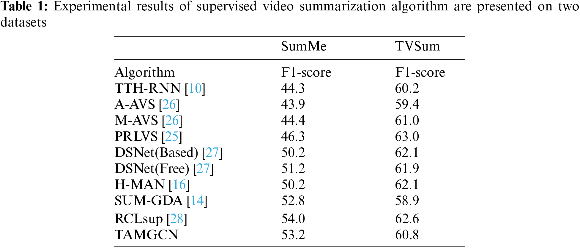
Table 2 compares the depth map-based video summarization method published in 2021. RSGN [21] firstly extracted the shot features and constructed the adjacency matrix, extracted the features through GCN, reconstructed the original video by constructing inverse GCN, and optimized the model through reinforcement learning. GCANsup [14] consists of two branches. One branch uses different scales to construct node features and adjacency matrix for video frames and uses GCN to extract structural features. The other branch uses dilated temporal convolution and temporal self-attention to extract video sequence features and finally uses the feature fusion mechanism. GAT [15] used LSTM to extract temporal features of videos by traditional methods. It then used VGG and spatial attention model to extract image features, construct graph attention network and generate weight factors. Results show that the algorithm in this paper achieves 60.8% on TVSum and 53.2% on SumMe.

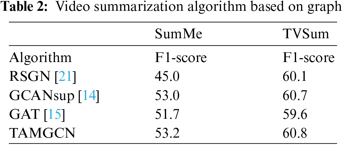
Table 3 shows the adjacency matrix construction by different algorithms. It can be seen from the table that different comparable results are obtained by constructing different adjacency matrices. It can be seen that the model proposed by us is robust to the function of constructing an adjacency matrix, and the adjacency matrix is constructed by using the most effective method. The adjacency matrix constructed by cosine similarity is better than the other three. In this case, it is used for the following comparison.

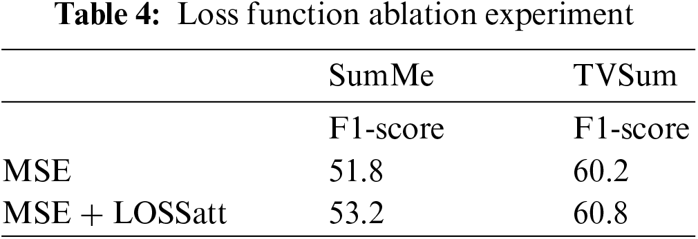
We conducted an additional experiment to investigate the validity of the loss function. When we trained our model method under supervision, the results reached 51.8% on the SumMe dataset and 60.2% on the TVSum dataset using the MSE loss optimization model. To verify the effectiveness of sparsity loss Lossatt, we used optimization model MSE + Lossatt and compared their results. As shown in Table 4, we found that using sparsity loss Lossatt could improve F1-score by 0.6% on the TVSum dataset and improve 1.4% on the SunMe dataset.

As shown in Figs. 5 and 6, although the predicted score is higher than the real score, on the whole, there is a strong correlation between the two scores on the whole. The real value is relatively consistent with the changing trend of the test paper, but the individual prediction is still not accurate.

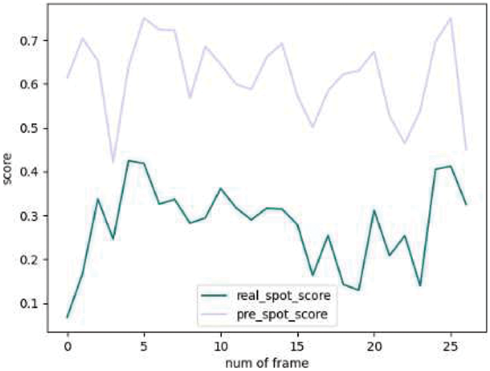
Figure 5: SumMe shot score comparison

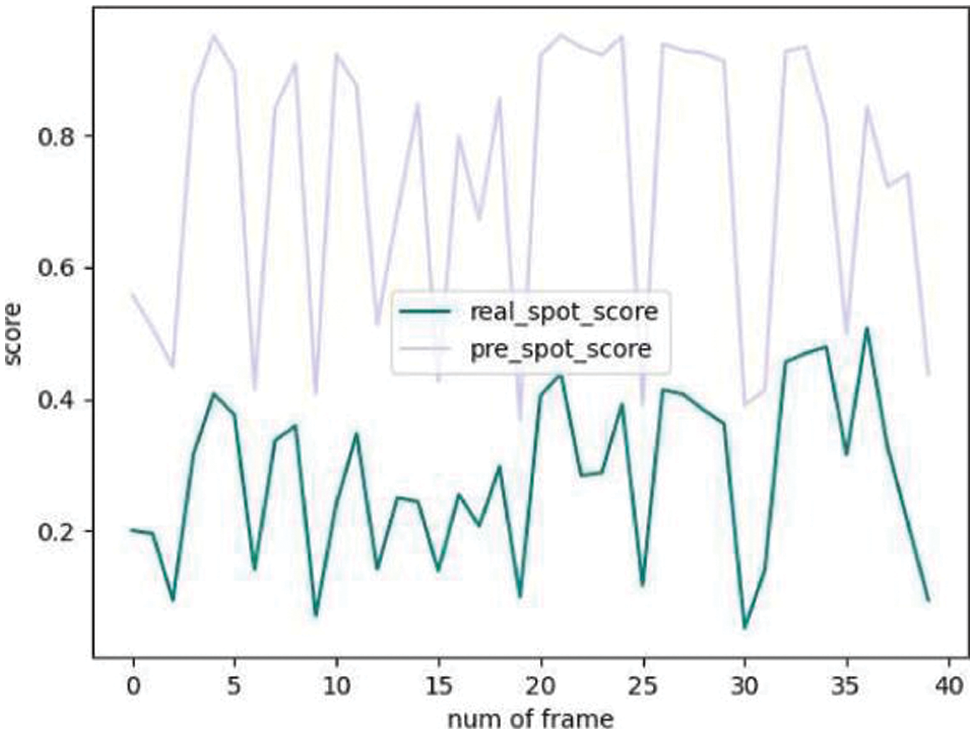
Figure 6: SumMe shot score comparison

As shown in Fig. 7, the adjacency matrix of the shots is displayed in a thermal diagram. Red represents the highest similarity, and white represents the lowest similarity. According to formula (24), it can be seen that the diagonal similarity of the adjacency matrix calculated according to the similarity is the highest, which proves from the side that the cosine distance between itself and itself is 1. From formula (25), it can be seen that the adjacency matrix is symmetric, so horizontally, the beginning and end of the video are similar, so the colour is similar in the thermal diagram. Fig. 8 shows the shots selected on the data set SumMe. From the captured images, it can be seen that the generated video summaries can describe the occurrence of the whole event in a relatively complete way.

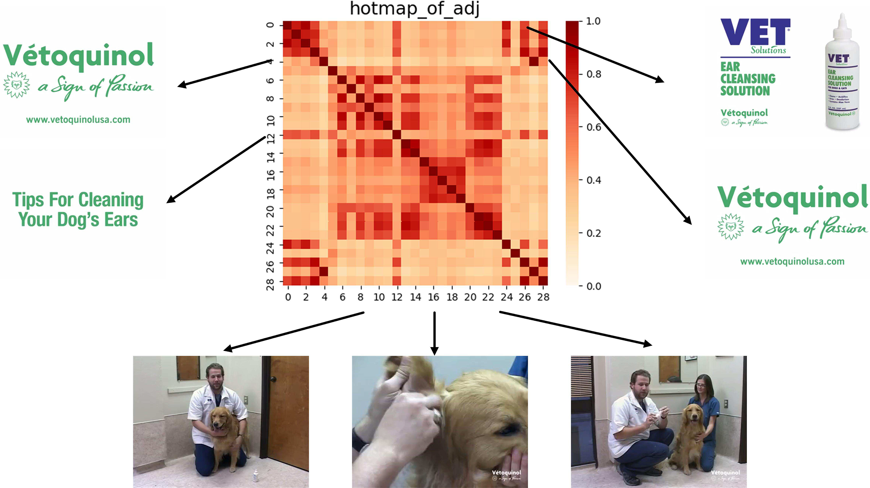
Figure 7: Example adjacency matrix

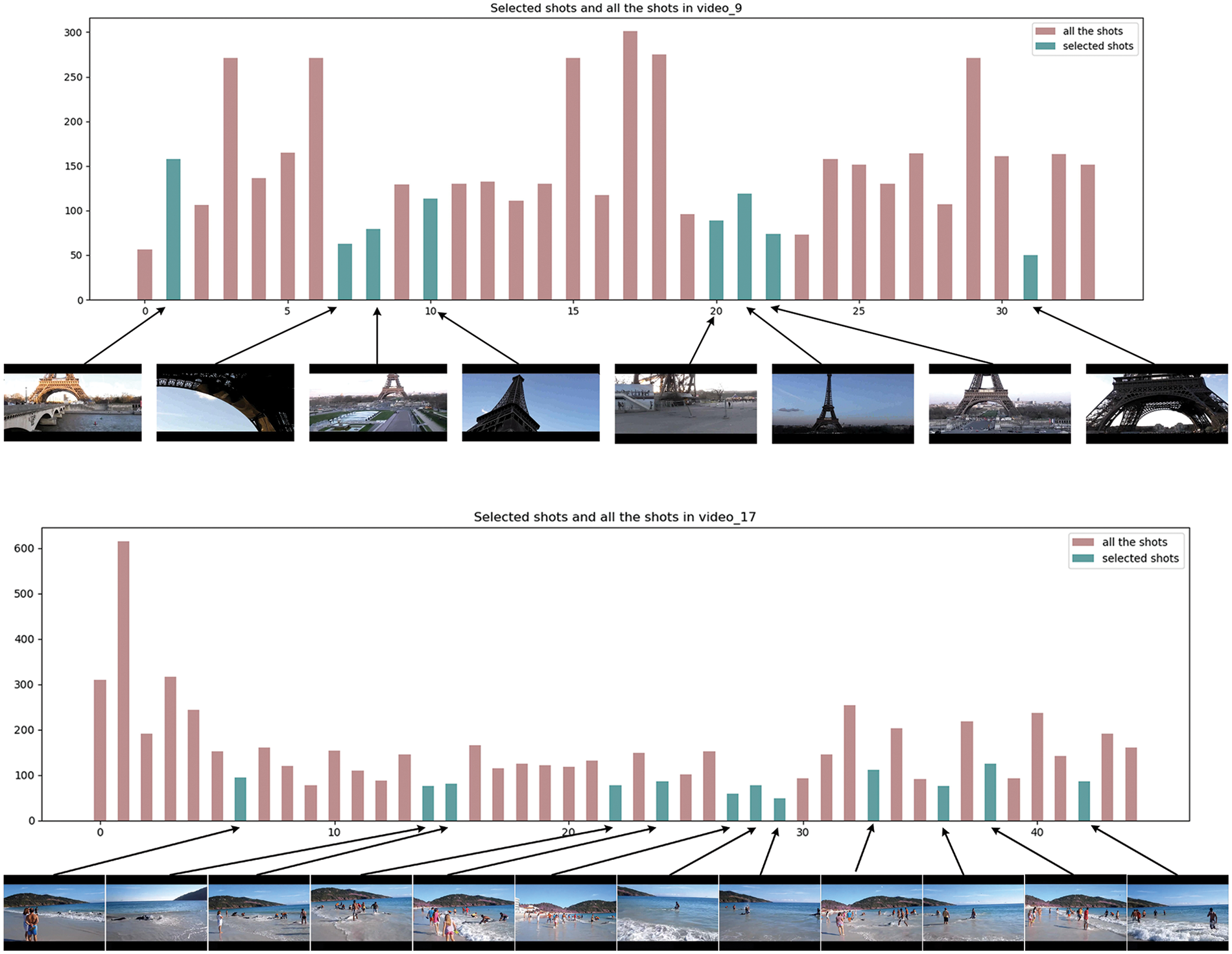
Figure 8: Importance score prediction

eij=f(xi,xi)=xiTxi||xi||2⋅||xi||2=1(24)

eij=f(xi,xj)=xiTxj||xi||2⋅||xj||2=xjTxi||xj||2⋅||xi||2=f(xjxi)=eji(25)

5  Conclusion

In this paper, we propose an adaptive graph convolutional adjacency matrix network for video summarization, with the goal of addressing the issue of fixed neighbor aggregation in graph neural network-based methods. The network first applies a graph convolutional network to extract the image features of each video frame. Next, the video is shot-cut, from which representative frames are selected to represent the entire shot. Then, the neighborhood matrix is constructed using the shot features as nodes and the similarity between shots as the weights of the edges. Subsequently, structural features are calculated using TAMGCN. During this process, the adjacency matrix is dynamically updated, a design that makes the adjacency matrix more reflective of the current graph structure and thus generates more representative summaries. Finally, the shot score is calculated by feature fusion. The introduction of feature fusion contributes to the preservation of the original features of the video frames. In addition, we design a sparse rule to train the network to induce the selection of different summaries. We conducted extensive experiments on the standard datasets SumMe and TVsum, and the experimental results proved the effectiveness of the model. However, the model may suffer from high memory consumption and difficulty in scaling when dealing with large-scale graph data. In future work, we intend to investigate models that are more adapted to handle large-scale graph data. In addition, we will focus on investigating multimodal video summarization models that use multiple sources of information such as audio, text, etc., to guide the model in generating high quality summaries. We will also delve into the interpretability of the model to better understand the decision-making process and outcomes of the model.

Acknowledgement: This work was supported by Natural Science Foundation of Gansu Province, Basic Research Program of Gansu Province, Gansu University of Political Science and Law Major Scientific Research and Innovation Projects, the Young Doctoral Fund Project of Higher Education Institutions in Gansu Province in 2022, Gansu Province Higher Education Innovation Fund Project, the University-Level Research Funding Project and University-Level Innovative Research Team of Gansu University of Political Science and Law.

Funding Statement: This work was supported by Natural Science Foundation of Gansu Province under Grant Nos. 21JR7RA570, 20JR10RA334, Basic Research Program of Gansu Province No. 22JR11RA106, Gansu University of Political Science and Law Major Scientific Research and Innovation Projects under Grant No. GZF2020XZDA03, the Young Doctoral Fund Project of Higher Education Institutions in Gansu Province in 2022 under Grant No. 2022QB-123, Gansu Province Higher Education Innovation Fund Project under Grant No. 2022A-097, the University-Level Research Funding Project under Grant No. GZFXQNLW022 and University-Level Innovative Research Team of Gansu University of Political Science and Law.

Author Contributions: The authors confirm contribution to the paper as follows: study conception and design: Jing Zhang, Guangli Wu; data collection: Shanshan Song; analysis and interpretation of results: Shanshan Song; draft manuscript preparation: Jing Zhang, Guangli Wu and Shanshan Song. All authors reviewed the results and approved the final version of the manuscript.

Availability of Data and Materials: We use SumMe and TVsum public datasets. The storage links are respectively SumMe Dataset | Papers With Code and yalesong/tvsum: TVSum: Title-Based Video Summarization dataset (CVPR 2015) (github.com).

Conflicts of Interest: The authors declare that they have no conflicts of interest to report regarding the present study.

References

1. P. Meena, H. Kumar, and S. K. Yadav, “A review on video summarization techniques,” Eng. Appl. Artif. Intell., vol. 118, no. 6, p. 105667, 2023. doi: 10.1016/j.engappai.2022.105667. [Google Scholar] [CrossRef]

2. V. Tiwari and C. Bhatnagar, “A survey of recent work on video summarization: Approaches and techniques,” Multimed. Tools Appl., vol. 2021, no. 80, pp. 27187–27221, 2021. doi: 10.1007/s11042-021-10977-y. [Google Scholar] [CrossRef]

3. D. Gupta and A. Sharma, “A comprehensive study of automatic video summarization techniques,” Artif. Intell. Rev., vol. 56, no. 10, pp. 11473–11633, 2023. doi: 10.1007/s10462-023-10429-z. [Google Scholar] [CrossRef]

4. P. Saini, K. Kumar, S. Kashid, A. Saini, and A. Negi, “Video summarization using deep learning techniques: A detailed analysis and investigation,” Artif. Intell. Rev., vol. 56, no. 11, pp. 12347–12385, 2023. doi: 10.1007/s10462-023-10444-0. [Google Scholar] [PubMed] [CrossRef]

5. X. Yan et al., “Video scene parsing: An overview of deep learning methods and datasets,” Comput. Vis. Image Underst., vol. 201, no. 1, p. 103077, 2020. doi: 10.1016/j.cviu.2020.103077. [Google Scholar] [CrossRef]

6. Q. Wang, L. Zhang, Y. Li, and K. Kpalma, “Overview of deep-learning based methods for salient object detection in videos,” Pattern Recognit., vol. 104, no. 12, p. 107340, 2020. doi: 10.1016/j.patcog.2020.107340. [Google Scholar] [CrossRef]

7. B. R. Kiran, D. M. Thomas, and R. Parakkal, “An overview of deep learning based methods for unsupervised and semi-supervised anomaly detection in videos,” J. Imaging, vol. 4, no. 2, p. 36, 2018. doi: 10.3390/jimaging4020036. [Google Scholar] [CrossRef]

8. C. Zhao, C. Hu, H. Shao, Z. Wang, and Y. Wang, “Towards trustworthy multi-label sewer defect classification via evidential deep learning,” in ICASSP 2023—2023 IEEE Int. Conf. Acoustics, Rhodes Island, Greece, Speech Signal Process. (ICASSP), IEEE, pp. 1–5. [Google Scholar]

9. E. Apostolidis, E. Adamantidou, A. I. Metsai, V. Mezaris, and I. Patras, “Video summarization using deep neural networks: A survey,” Proc. IEEE, vol. 109, no. 11, pp. 1838–1863, 2021. doi: 10.1109/JPROC.2021.3117472. [Google Scholar] [CrossRef]

10. B. Zhao, X. Li, and X. Lu, “TTH-RNN: Tensor-train hierarchical recurrent neural network for video summarization,” IEEE Trans. Ind. Electron., vol. 68, no. 4, pp. 3629–3637, 2020. doi: 10.1109/TIE.2020.2979573. [Google Scholar] [CrossRef]

11. M. Hu, R. Hu, Z. Wang, Z. Xiong, and R. Zhong, “Spatiotemporal two-stream LSTM network for unsupervised video summarization,” Multimed. Tools Appl., vol. 81, no. 28, pp. 40489–40510, 2022. doi: 10.1007/s11042-022-12901-4. [Google Scholar] [CrossRef]

12. J. Lin, S. Zhong, and A. Fares, “Deep hierarchical LSTM networks with attention for video summarization,” Comput. Electr. Eng., vol. 97, no. 7, pp. 107618, 2022. doi: 10.1016/j.compeleceng.2021.107618. [Google Scholar] [CrossRef]

13. J. Wu, S. Zhong, and Y. Liu, “Dynamic graph convolutional network for multi-video summarization,” Pattern Recognit., vol. 107, no. 1, pp. 107382, 2020. doi: 10.1016/j.patcog.2020.107382. [Google Scholar] [CrossRef]

14. P. Li, C. Tang, and X. Xu, “Video summarization with a graph convolutional attention network,” Front. Inf. Technol. Electron. Eng., vol. 22, no. 6, pp. 902–913, 2021. doi: 10.1631/FITEE.2000429. [Google Scholar] [CrossRef]

15. R. Zhong, R. Wang, Y. Zou, Z. Hong, and M. Hu, “Graph attention networks adjusted Bi-LSTM for video summarization,” IEEE Signal Process. Lett., vol. 28, pp. 663–667, 2021. doi: 10.1109/LSP.2021.3066349. [Google Scholar] [CrossRef]

16. Y. T. Liu, Y. J. Li, F. E. Yang, S. F. Chen, and Y. C. F. Wang, “Learning hierarchical self-attention for video summarization,” in 2019 IEEE Int. Conf. Image Process. (ICIP), Taipei, Taiwan, IEEE, Sep. 2019, pp. 3377–3381. [Google Scholar]

17. G. Liang, Y. Lv, S. Li, S. Zhang, and Y. Zhang, “Video summarization with a convolutional attentive adversarial network,” Pattern Recognit., vol. 131, no. 6, pp. 108840, 2022. doi: 10.1016/j.patcog.2022.108840. [Google Scholar] [CrossRef]

18. X. Hu, X. Hu, J. Li, and K. You, “Generative adversarial networks for video summarization based on key-frame selection,” Inf. Technol. Control., vol. 52, no. 1, pp. 185–198, 2023. doi: 10.5755/j01.itc.52.1.32278. [Google Scholar] [CrossRef]

19. R. Panda, A. Das, Z. Wu, J. Ernst, and A. K. Roy-Chowdhury, “Weakly supervised summarization of web videos,” in Proc. IEEE Int. Conf. Comput. Vis., Venice, Italy, 2017, pp. 3657–3666. [Google Scholar]

20. H. I. Ho, W. C. Chiu, and Y. C. F. Wang, “Summarizing first-person videos from third persons’ points of view,” in Proc. Eur. Conf. Comput. Vis. (ECCV), Munich, Germany, 2018, pp. 70–85. [Google Scholar]

21. B. Zhao, H. Li, X. Lu, and X. Li, “Reconstructive sequence-graph network for video summarization,” IEEE Trans. Pattern Anal. Mach. Intell., vol. 44, no. 5, pp. 2793–2801, 2021. doi: 10.1109/TPAMI.2021.3072117. [Google Scholar] [PubMed] [CrossRef]

22. W. Zhu, Y. Han, J. Lu, and J. Zhou, “Relational reasoning over spatial-temporal graphs for video summarization,” IEEE Trans. Image Process., vol. 31, pp. 3017–3031, 2022. doi: 10.1109/TIP.2022.3163855. [Google Scholar] [PubMed] [CrossRef]

23. J. Park, J. Lee, I. J. Kim, and K. Sohn, “SumGraph: Video summarization via recursive graph modeling,” in Comput. Vis.–ECCV 2020: 16th Eur. Conf., Glasgow, UK, Springer International Publishing, Aug. 23–28, 2020, vol. 16, pp. 647–663. [Google Scholar]

24. T. Psallidas and E. Spyrou, “Video summarization based on feature fusion and data augmentation,” Computers, vol. 12, no. 9, pp. 186, 2023. doi: 10.3390/computers12090186. [Google Scholar] [CrossRef]

25. G. Wang, X. Wu, and J. Yan, “Progressive reinforcement learning for video summarization,” Inf. Sci., vol. 655, p. 119888, 2024. doi: 10.1016/j.ins.2023.119888. [Google Scholar] [CrossRef]

26. Z. Ji, K. Xiong, Y. Pang, and X. Li, “Video summarization with attention-based encoder-decoder networks,” IEEE Trans. Circuits Syst. Video Technol., vol. 30, no. 6, pp. 1709–1717, 2019. doi: 10.1109/TCSVT.2019.2904996. [Google Scholar] [CrossRef]

27. W. Zhu, J. Lu, J. Li, and J. Zhou, “DSNet: A flexible detect-to-summarize network for video summarization,” IEEE Trans. Image Process., vol. 30, pp. 948–962, 2020. doi: 10.1109/TIP.2020.3039886. [Google Scholar] [PubMed] [CrossRef]

28. Y. Zhang, Y. Liu, P. Zhu, and W. Kang, “Joint reinforcement and contrastive learning for unsupervised video summarization,” IEEE Signal Process. Lett., vol. 29, pp. 2587–2591, 2022. doi: 10.1109/LSP.2022.3227525. [Google Scholar] [CrossRef]