A Hybrid Deep Learning and Machine Learning-Based Approach to Classify Defects in Hot Rolled Steel Strips for Smart Manufacturing

1  Introduction

The standards for product quality have increased as a result of the development of smart manufacturing. Hot-rolled steel strips are a main product in the manufacturing industry, used in a variety of industries’ production processes [1]. Rolling the billet until it reaches a temperature greater than that recrystallization temperature is the first step in the hot-rolled steel strip manufacturing process. Other phases include edge cutting, straightening, polishing, and phosphorus elimination [2]. The resultant hot-rolled steel strips have strong covering capabilities and good processing performance. These days, steel strips are used in many industries, including the automobile, home appliance, shipbuilding, chemical, and electric motor industries, as well as in everyday life and industrial operations [2–5].

One of the main factors affecting steel strips’ ability to compete in the market is their surface quality. Since hot-rolled steel strips are essential parts of many different products, it is crucial to classify and identify surface defects in steel during the production process as part of quality control. Due to a variety of metallurgical and mechanical imperfections, surface defects on steel plates are a major source of concern in the industrial manufacturing process. In the manufacturing process, various defects can occur on steel surfaces. These include crazing, inclusions, rolled-in scale, patches, scratches, pitted surfaces, and other abnormalities [5–7], which not only impact the visual appearance of steel plates but also affect their fatigue strength [8]. The steel plate’s strength and resistance to corrosion suffer significantly from these issues, impacting the economic returns of the factory. Failing to address these defects promptly can lead to a decline in the quality of the steel products, with repercussions not only on the manufacturers’ reputation and financial losses but also on the safety and reliability of the end-user’s products [5,6]. Therefore, it becomes necessary to identify these surface defects and monitor the industrial process [9] to improve the surface quality of the steel strips.

Traditionally, defect detection of steel surfaces has relied on manual inspection, which is both inefficient and unreliable. The main technique for defect detection was manual labor, which used the workers’ eyes and experience to classify and find the defects [7]. This approach performs poorly in real-time and has a high false detection rate. Under ideal working conditions, only about 80% of even the most skilled and knowledgeable personnel can detect surface imperfections. This not only led to inefficiencies but also raised the risk of incorrect and overlooked detections. Therefore, it becomes necessary to systematically classify and identify these surface defects. The detection system for steel strips is currently widely utilized in modern steel plants, as shown in Fig. 1.

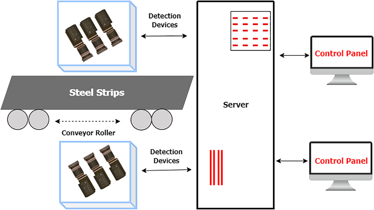
Figure 1: The system for detecting surface defects on steel strips

As shown in Fig. 1, the conveyor rollers rotate the strips through the detection device. Detection devices usually consist of protective devices, light sources, and industrial cameras. When strips rotate through the detection device, it captures high-speed images of steel strips, and these images are then sent to the server for algorithmic processing. After extracting samples, the server sends them to the control panel for inspection and later examination [2]. The existing detection system’s hardware requirements are suitable for detection; however, the classification algorithm on the server needs to be updated to achieve better classification results for steel strip defect detection.

Classification is a supervised machine learning approach used to solve various problems [2,10]. In recent times, with advancements in Computer Vision (CV) [11] and Artificial Intelligence (AI) technologies, various types of Statistical [12,13], Machine Learning (ML) [13,14], and Deep Learning (DL) [2,4,5,15] methods have been developed for feature extraction and automatic classification of steel surface defects. However, despite these developments, none of these methods can achieve outstanding performance across all problems and scenarios due to insufficient and imbalanced data. The main objective of this study is to deal with the issue of low accuracy in automatically classifying surface defects on steel strips by utilizing a hybrid deep learning model. In order to achieve this, we first applied offline image augmentation techniques to balance and augment the dataset. Then, we utilized the pre-trained VGG19 model as a feature extractor along with an SVM classifier.

Unlike earlier studies, our suggested approach uses extensive and balanced datasets rather than limited and imbalanced datasets. This study’s key contributions include the following:

•   We proposed a hybrid deep learning model with global average pooling (GAP) and SVM classifier for accurately classifying steel strip defects with high performance.

•   To balance and expand the dataset size, various offline image augmentation techniques were applied to improve model robustness and accuracy.

•   The proposed system is compared to other recent research in order to show the performance of the proposed methodology in comparison to other available methodologies.

The remaining sections of the paper are organized as follows: Section 2 provides an overview of related works, including conventional machine learning-based approaches as well as deep learning-based approaches. Section 3 outlines the methodology, including details of the dataset used and the proposed model. Section 4 covers the results, discussion, experimental setup, and evaluation metrics. In Section 5, the study’s conclusions are presented along with possible directions for future research.

2  Related Works

The related work on steel surface defect classification can be categorized into two main approaches: conventional machine learning-based approaches, and deep learning-based approaches.

2.1 Conventional Machine Learning-Based Approaches

Several studies have tackled the shortcomings of manual visual examination by utilizing conventional machine learning (ML) techniques. Conventional ML-based approaches for surface defect identification involve two basic phases: feature extraction and classification [5]. Many techniques, such as local binary pattern [13], grey level co-occurrence matrix [16], and histogram of oriented gradients, have been used over the years to extract features. Next, the collected features are passed into a classifier, such as RF, KNN, and SVM, for defect classification [5].

Karthikeyan et al. [14] suggested using discrete wavelet transform-based local configuration pattern features as the input to be fed into the k-nearest neighbor classifier for defect classification, resulting in a 96.7% total accuracy. By altering the threshold pattern of the completed LBP, Song et al. [12] presented an adjacent evaluation of completed local binary patterns and support vector machines to classify NEU dataset defects. Hu et al. [17] identified four types of visual features: geometric features, form features, texture features, and grey-scale features. An SVM classifier and a hybrid chromosomal genetic approach were used to create a classification model that outperformed the traditional SVM model in terms of average prediction accuracy. Jiang et al. [18] presented an adaptive classifier using a bayes kernel that updates the model with small data to adapt for accuracy loss. Initially, various features were introduced in order to cover a huge amount of information about the defects. Second, they used the random feature subspace to construct a series of SVMs. Finally, they provided an updated mechanism for the bayes evolutionary kernel, and the basis SVM results were fused using a bayes classifier trained as an evolutionary kernel. Martins et al. [19] presented an automatic system based on two well-known feature extraction techniques: principal component analysis and self-organizing maps. This system uses Hough Transform, an image analysis technique, to classify three defects with well-defined geometric shapes: welding, clamp, and identification hole. The system was effectively validated, yielding an 87% overall accuracy rate.

The defect classification technique based on machine learning has produced good results that can be used to guide the actual production process. However, some traditional methods have various drawbacks in challenging situations since they rely on human feature extractions that require domain specialists, which can be a difficult process in some applications and often results in low classification accuracy. With massive and complicated data, conventional machine learning-based algorithms reach their limits in terms of accuracy. Furthermore, new detection tasks require the redesign of new algorithms, making algorithm migration challenging to solve a similar problem.

2.2 Deep Learning-Based Approaches

In recent years, deep learning-based CNN models and their variants [2,20–22] have recently beaten traditional machine learning methods for classifying defects in the steel industry. Convolutional Neural Networks (CNN) [23,24] models’ success and powerful feature extraction capabilities in CV related tasks have inspired researchers to apply them to different problems, such as image classification [2], object detection [8,25], and image segmentation [26].

Currently, researchers commonly use two different datasets for identifying defects in steel strips: the NEU surface defect (NEU-CLS) [12] dataset and the Xsteel surface defect dataset (XSDD) [21] dataset. Numerous high-level studies have been conducted based on the NEU surface defect (NEU-CLS) dataset, such as Lee et al. [20] described a unique methodology for diagnosing steel faults that employ a deep structured neural network, namely a CNN, as well as class activation maps with 99.44% accuracy. Jain et al. [27] introduced a GAN-based method to produce synthetic data for fine-tuning a pre-trained CNN for the NEU dataset, achieving an accuracy of 99.11%. Bouguettaya et al. [5] proposed a deep learning-based algorithm to classify six common surface defects in steel strips. With the use of transfer learning, they investigated the performance of two modern CNN architectures, Xception and MobileNet-V2, and achieved an accuracy of 99.72%. Ibrahim et al. present a novel approach to improving the accuracy of steel strip defect classification by integrating a pre-trained VGG16 model as a feature extractor and a new CNN as a classifier, resulting in a classification accuracy of 99.44% [28].

Several high-level studies have been conducted based on the Xsteel surface defect (XSDD) dataset, such as the Feng et al. [21] proposed (X-SDD) dataset in this study, which includes 1360 defect images total and seven common types of defects in a hot-rolled strip. To confirm the impact on the X-SDD, they use the recently suggested RepVGG algorithm combined with the spatial attention (SA) mechanism. On the test set, they achieved a 95.10% accuracy rate. In this study, Feng et al. [2] proposed a strip defect classification strategy for the X-SDD dataset that is based on ResNet50 and includes FcaNet and the convolutional block attention module. Hao et al. proposed a classification strategy in this study by merging generative adversarial networks (GAN) with attention mechanisms. They developed a unique data augmentation method, the WGAN model, to create new surface defect images. Second, to detect defects, a Multi-SE-ResNet34 model with an attention mechanism is presented to identify steel defects [29]. Zheng et al. proposed a method combining Legendre multi-wavelet transform and autoencoder network (LWT-AE) for the classification of steel surface defects, achieving a classification accuracy of 95.37% [30].

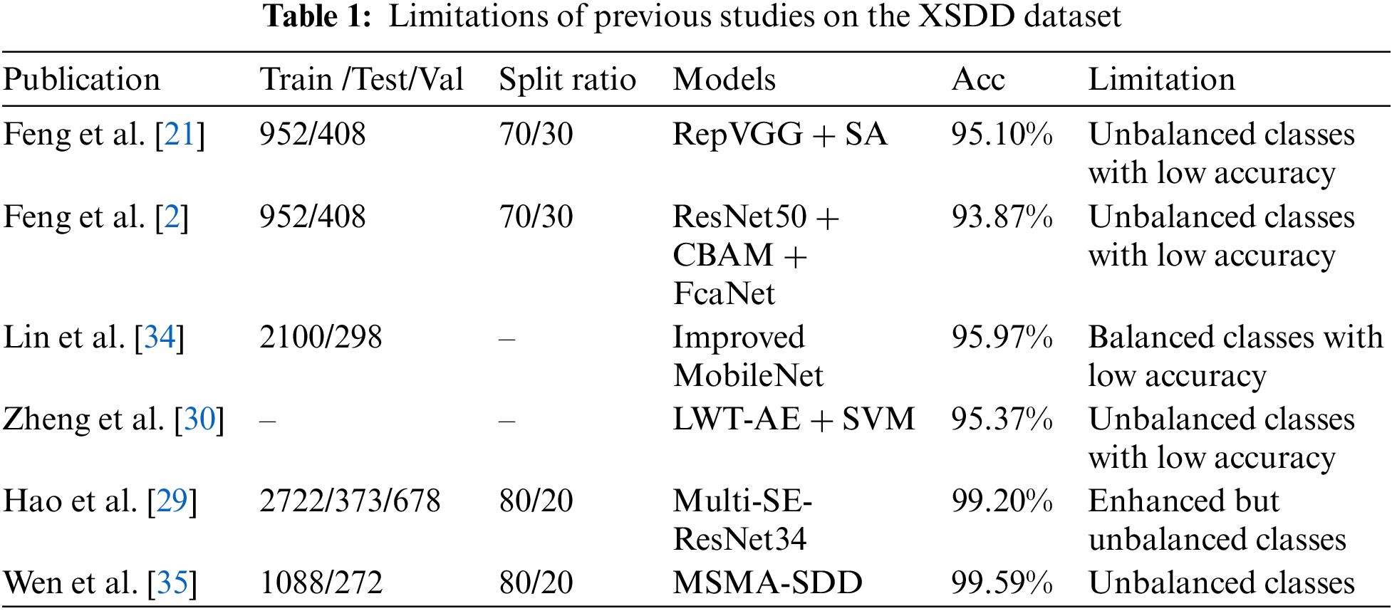
Previous research has proven that the DL-based classification algorithms for steel strip surface defects are effective. However, there are still problems with current research. First, earlier studies used unbalanced XSDD datasets, which do not produce ideal results [31] because many classification algorithms neglect or misclassify examples of the minority class in order to focus on the majority class [32], and second, the quality and size of training samples have a significant impact on the performance of the DL model [33]. Table 1 shows the limitations and problems with existing techniques.

3  Methodology

This section describes the procedures for gathering and enhancing data, the creation of a hybrid ML and DL-based model, the setup of our experiments, and the performance evaluation matrices that were employed in the experiment. As shown in Fig. 2, the general methodology of the system includes image dataset acquisition, pre-processing and offline augmentation, data preparation for training and test set, feature extraction, and classification.

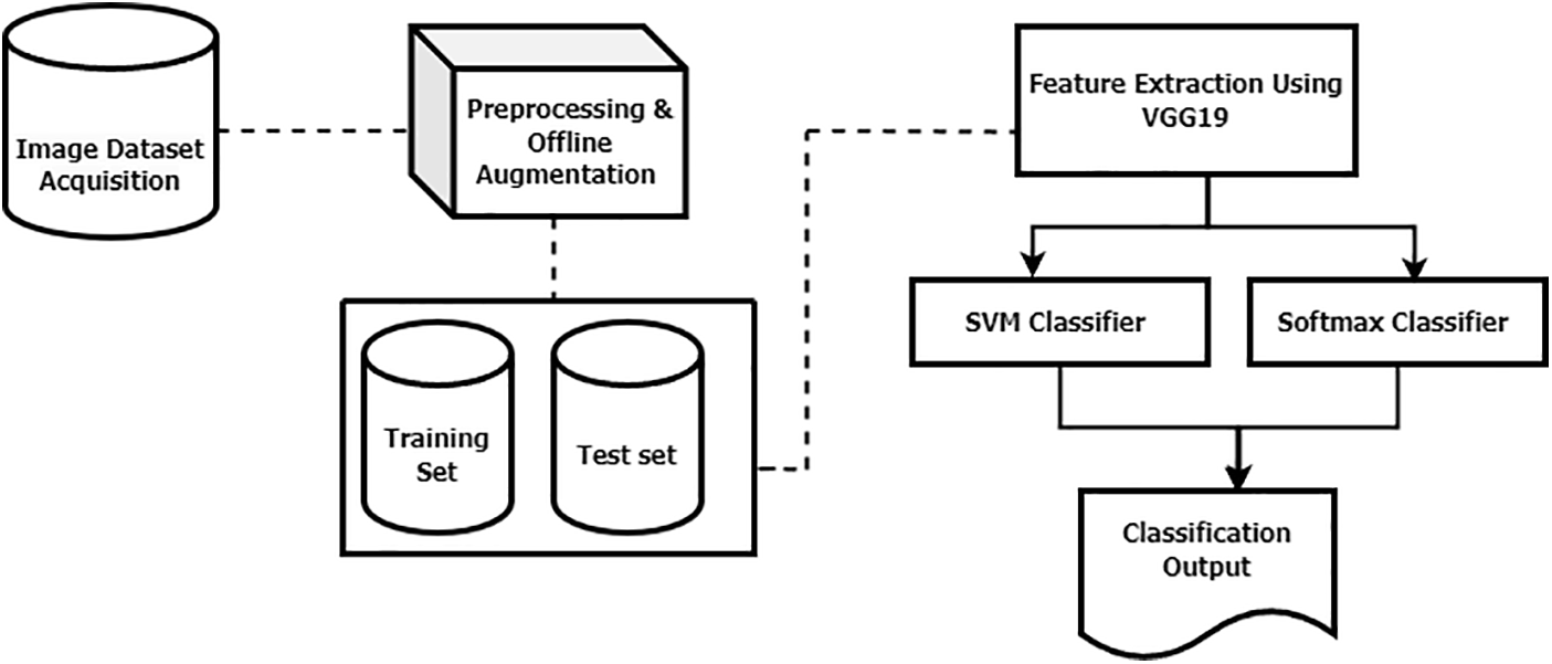
Figure 2: General methodology of the system

3.1 Details of the Dataset

The proposed methodology has been evaluated with two distinct data sets, namely the NEU-CLS surface defect dataset and the Xsteel surface defect dataset, as described in the sections that follow.

3.1.1 The NEU Surface Defect (NEU-CLS)

The dataset used in this study comes from the NEU database, which was developed by Northeast University in China. It consists of six types of different surface defects on a hot-rolled steel strip: patches, crazing, inclusion, pitted_surface, scratch, and rolled_in_scale [12]. Each type of defective hot rolled strip surface consists of 300 images, totaling 1800 images in this dataset. Each image’s original pixel resolution is 200 × 200. We resize images to 224 × 224 × 3 according to the requirements of my model. Each class in the dataset is shown in detail in Fig. 3.

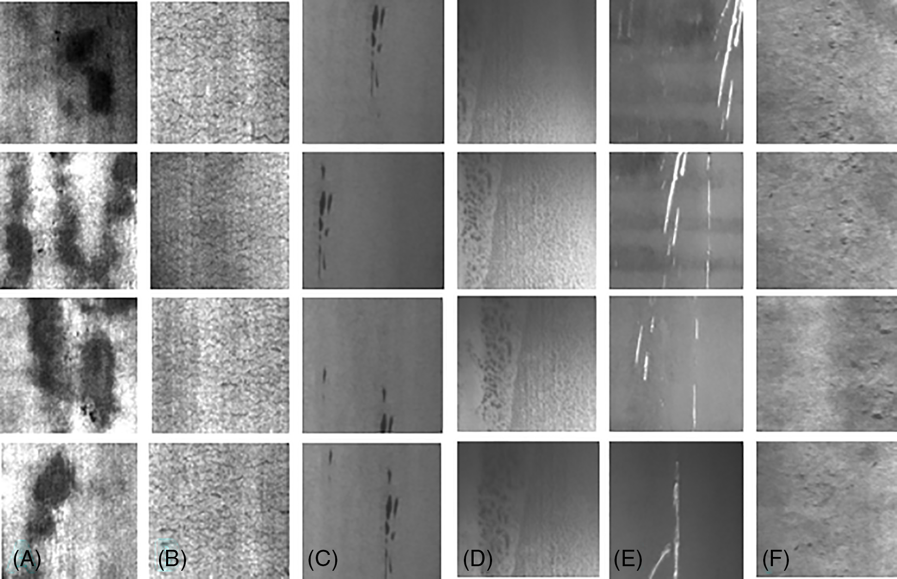
Figure 3: Sample images of six types of surface defects on NEU-CLS dataset (A) patches (B) crazing (C) inclusion (D) pitted_surface (E) scratches (F) rolled_in_scale

3.1.2 The Xsteel Surface Defect Dataset (XSDD)

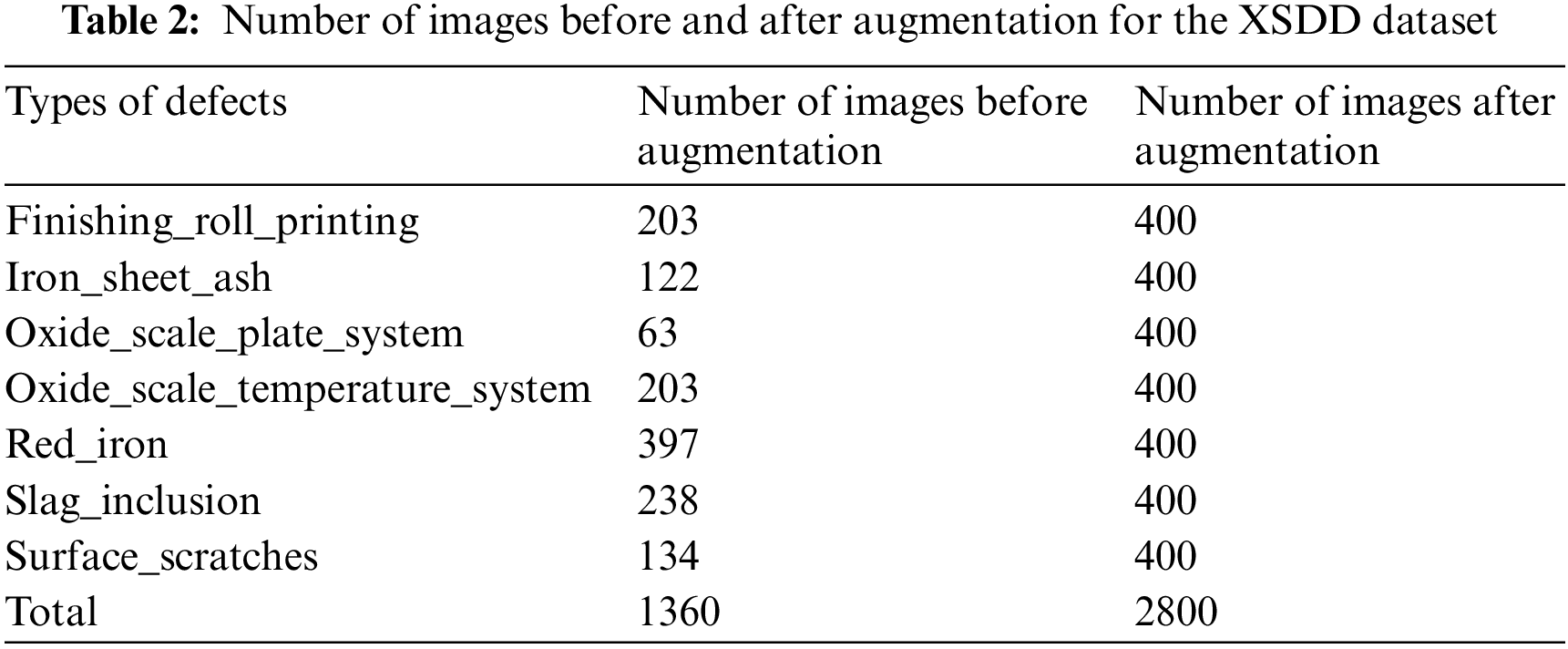
The XSDD dataset of hot-rolled steel strips is a recently published dataset to classify and detect steel surface defects in the field of academic research [21]. The XSDD collection includes 1360 defective images that cover seven types of different surface defects on a hot-rolled steel strip, including 203 images of finishing roll printing, 122 images of iron sheet ash, 63 images of oxide scale-of-plate system, 203 images of oxide scale of temperature system, 397 images of red iron sheet, 238 images of slag inclusions, and 134 images of surface scratches. Each image’s original pixel resolution is 128 × 128. We resize images to 224 × 224 × 3 according to the requirements of my model. Each class in the dataset is shown in detail in Fig. 4.

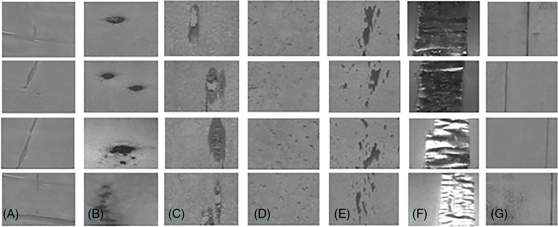
Figure 4: Sample images of seven types of surface defects on the X-SDD dataset (A) finishing_roll_printing (B) iron_sheet_ash (C) oxide_scale_plate_system (D) oxide_scale_temperature_system (E) red_iron (F) slag_inclusion (G) surface-scratches

3.1.3 Dataset Augmentation

Data augmentation is a strategy for increasing the size of data artificially with the aim of improving the ability to generalize the model and reduce overfitting [36]. In this research, offline data augmentation is employed on both datasets as a preprocessing step to balance and enhance the size of the dataset. The Python PIL library is utilized to perform various transformations on a collection of images. The augmentation process involves applying horizontal and vertical flips, along with rotations of 5°, 10°, 15°, and 20° to random images, which is the best combination of augmentation techniques for various surface defects datasets [37,38]. This flipping and rotation strategy enhances the model’s robustness. We expanded the NEU-CLS dataset from 1800 to 2400 and the XSDD dataset from 1360 to 2800 images, ensuring a balanced representation with 400 images for each class. Fig. 5 displays some examples of the augmented images. Table 2 provides the details of the dataset before and after augmentation for the XSDD dataset while Table 3 provides the details of the dataset before and after augmentation for the NEU-CLS dataset.

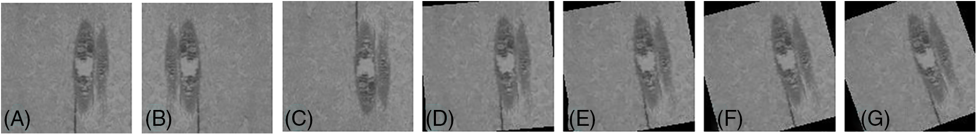
Figure 5: Samples of offline-augmented images (A) original (B) horizontal_flip (C) vertical_flip (D) 5° rotation (E) 10° rotation (F) 15° rotation (G) 20° rotation

3.2 Proposed Hybrid Deep Learning (DL) Model

Convolutional Neural Network (CNN) is a traditional DL-based approach in the field of computer vision. Its design is influenced by how human brains process visual information. The convolutional layer, pooling layer, and fully-connected (FC) layer are the three main layers of a CNN. CNNs outperform traditional neural networks due to their weight sharing feature, reducing parameters, and improving generalization. They efficiently combine feature extraction and classification, leading to structured, feature-dependent model outputs. For large-scale implementations, CNNs are the preferred choice, simplifying the process [39]. The main challenges with convolutional neural networks are their work on large datasets for training and the need for long time with GPU support. To deal with the large dataset problem, transfer learning is used [28,40,41]. The transfer learning approach involves training a pre-trained model on a large ImageNet [42] dataset, which has more than a million images with thousands of classes [41,43], and then applying it to the specified task of interest. By reusing a pre-trained CNN in this way, the deep CNN can effectively handle small dataset problems in different domains.

3.2.1 Visual Geometry Group (VGG19) Based CNN Model

Simonyan et al. introduced the Visual Geometry Group (VGG19) [44], which is a convolutional neural network comprising a total of 19 layers, including 16 convolution layers and 3 fully connected layers. The required input size for VGG19 is 224 × 224 in order to process it. The network employs 16 convolutional layers for feature extraction, with the subsequent 3 layers dedicated to classification tasks. All convolution layers within VGG19 utilize a 3 × 3 filter, and the layers used for feature extraction are organized into 5 groups, with each group followed by max-pooling layers. The dimensions of the final feature map, including width, height, and depth, are influenced by both the architecture of the neural network and the pooling layers employed. In our case, we utilized a convolutional layer with a 3 × 3 kernel size and max pooling with a 2 × 2 kernel size, which plays an essential role in determining the dimensions of the feature map. In this study, we used VGG19 as a backbone to extract features from images of steel defects. The architecture of the original Visual Geometry Group (VGG19) is shown in Fig. 6.

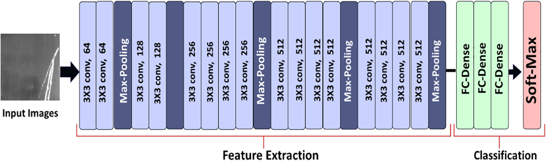
Figure 6: Architecture of original visual geometry group (VGG19) model

3.2.2 Support Vector Machine (SVM)

In supervised learning, SVM is frequently employed, especially for problems involving binary classification. However, in this study, we need to extend its functionality to handle multi-class classification. Specifically, we aim to use a multi-class SVM to classify different classes of steel surface defect images. For this purpose, we employed L2-SVM multi-class classifiers with the Squared Hinge Loss (SHL).

The L2-SVM optimizes the L2 norm and employs the Squared Hinge Loss (SHL). This loss function minimizes the Euclidean norm while imposing a significant penalty for errors. Eq. (1) presents the formulation of the L2-SVM, which is a popular variant that minimizes the squared hinge loss [45,46].

minimize 1P‖w‖22+C∑i=1Pmax (0,1−yi′(WTxi+b))2(1)

In this equation, WT represents the weight of the dataset, and WTxi+b serves as the predictor function. The actual class is represented by y′ and the predicted class is represented by y. ‖w‖2 represents the Euclidean norm (also known as the L2 norm), along with the squared hinge loss. The parameter C denotes the large error penalty for misclassification, where C > 0.

3.2.3 Global Average Pooling

To get the base model ready for the final classification layer, we included Global Average Pooling (GAP) [47]. GAP calculates the mean result of every feature map from the previous layer without adding new trainable parameters. This layer significantly contributes to data reduction and aids in stabilizing validation accuracy. When GAP is combined with the base model, overfitting is reduced, and the CNN model’s overall calculation time is decreased. The GAP layer transforms a feature map into a single map by averaging all its values. This layer reduces the spatial dimensions of a tensor represented as H × W × D to a tensor with dimensions of 1 × 1 × D, as shown in Fig. 7.

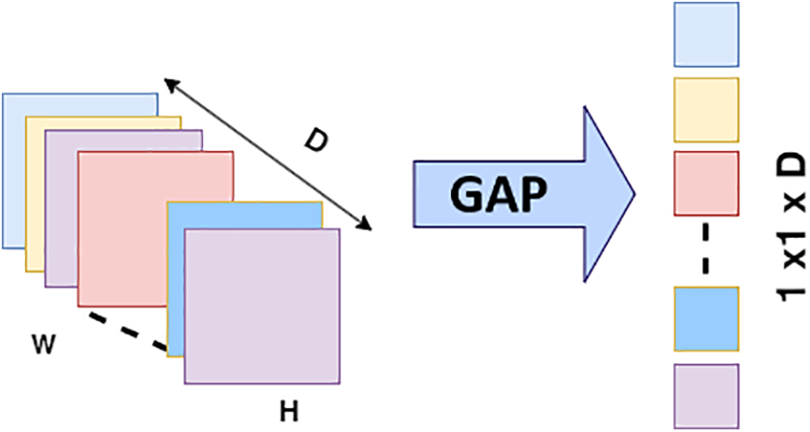
Figure 7: Global average pooling (GAP)

3.2.4 Construction of Proposed Hybrid Model

The proposed approach classifies steel surface defects by combining a pre-trained CNN with the machine learning algorithm SVM [48]. Researches [45,49] show that a hybrid CNN performs superior to a standard CNN. In the present work, we utilized the TL-based Visual Geometry Group 19 (VGG19) [44] model as a backbone to extract features. As shown in Fig. 8a, “Step 1” refers to the feature extraction layers, and “Step 2” refers to classification.

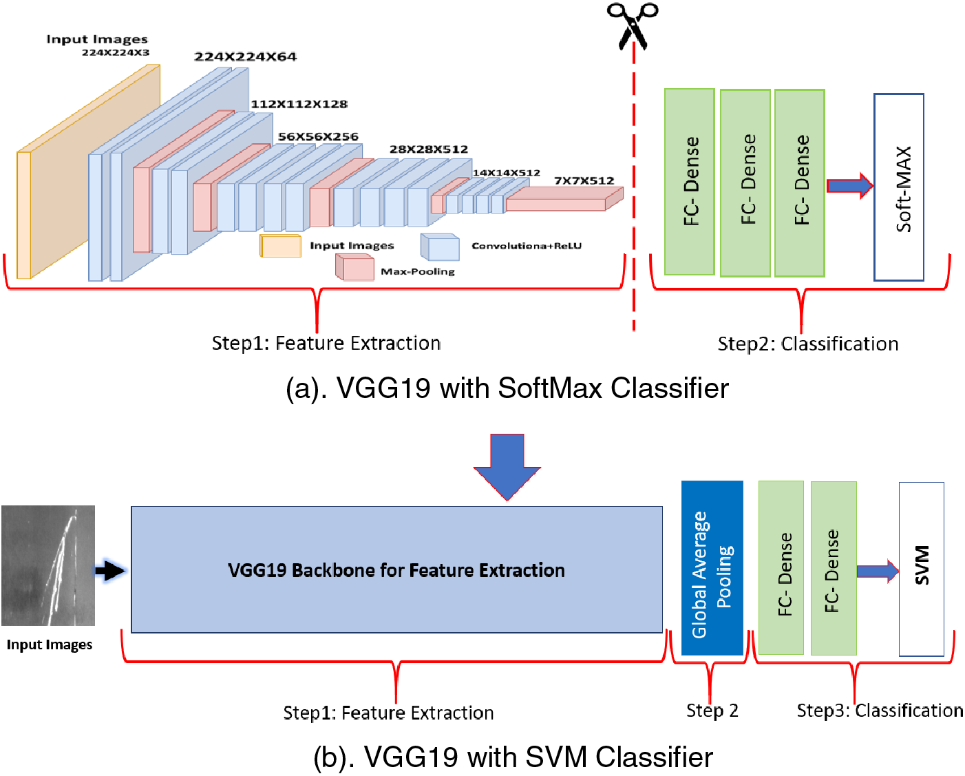
Figure 8: A proposed hybrid model based on VGG19 and SVM

To create a hybrid model, we removed the classification part of the VGG19 model, as shown in Fig. 8a, and included a Global Average Pooling layer. Further, we added FC layers and SVM as a classifier, as shown in Fig. 8b. As shown in Fig. 8b, “Step 1” refers to the feature extraction layers, “Step 2” refers to Global Average Pooling, and “Step 3” refers to classification. In Step 2, the Global Average Pooling (GAP) [47] layer efficiently reduces the height and width of the input into a single vector, resulting in a significant dimensionality reduction. This process helps to reduce model overfitting.

The VGG19-based CNN model utilized the Softmax activation function for classifying the final output in its last layer. On the other hand, the proposed hybrid VGG19-based SVM model took a different approach by employing the SVM classifier instead of the Softmax activation function, as illustrated in Fig. 8b.

4  Results, Discussion, and Experimental Setup

This section presents the results obtained by the proposed model for classifying steel defects and the experimental setup used to perform the experiments.

4.1 Experiment Setting

The dataset is divided into an 80:20 split ratio for training and testing. We have standardized the input size to 224 × 224 × 3 pixels. For the NEU-CLS dataset, which consists of a total of 2400 images (400 images for each class) after augmentation, we used a total of 1920 images (320 images for each class) as a training set and 480 images (80 images for each class) as a testing set. Similarly, for the XSDD dataset, which consists of a total of 2800 images (400 images for each class) after augmentation, we used a total of 2240 images (320 images for each class) as a training set and 560 images (80 images for each class) as a testing set.

For carrying out all experiments, we utilized an AMD Ryzen 7 2700X Eight-Core Processor (3.70 GHz) along with a Nvidia GeForce RTX 2080Ti. Furthermore, the code was implemented in a Jupiter Notebook environment using the anaconda platform with TensorFlow 2.10.0 and Python 3.9.18 version. In our experiment, we set the batch size to 32, and the learning rate is between 0.001–0.0001 based on the experiments, which showed training stability. Optimization was done using the Adam optimizer, and the squared hinge loss was used as a loss function. We conducted training over 100 epochs. Through experiments, we found that this combination of hyperparameters yielded the best results for steel defect classification. The details of the settings used in the model’s implementation are shown in Table 4.

4.2 Evaluation Metrics

We assessed the efficiency of our proposed methodology for classifying steel surface defects through various metrics. Our evaluation included metrics of measurement such as accuracy, macro recall, macro precision, and macro F1-score, providing a comprehensive understanding of the model’s effectiveness in handling various aspects of the classification task. Accuracy, Macro Precision, Macro Recall, and Macro F1-score are calculated using the following equations, as shown in Eqs. (2)–(5).

Accuracy=TP+TNTP+TN+FP+FN(2)

MacroRecall=1N∑i=1NTPiTPi+FNi(3)

MacroPrecision=1N∑i=1NTPiTPi+FPi(4)

MacroF1−score=1N∑i=1N2×Precission(i)∗Recall(i)Precission(i)+Recall(i)(5)

where FN represents a false negative, TP represents a true positive, TN represents a true negative, and FP represents a false positive. It measures the overall performance of the classification model, and N is the total class of defect types. Accuracy is the percentage of correct predictions among all the samples that were tested. Precision quantifies the accuracy of positive predictions, while recall evaluates the model’s ability to correctly identify all positive instances. The F1-score, calculated as the harmonic mean of precision and recall, provides a balanced measure of both metrics. A score of 1 indicates the highest performance, while the worst score is 0. The trade-off between precision and recall is a challenge in imbalanced classes. Accuracy and F1-score may not accurately reflect performance in imbalanced datasets due to biases towards the majority class, but our model achieved good results due to the balanced nature of the dataset.

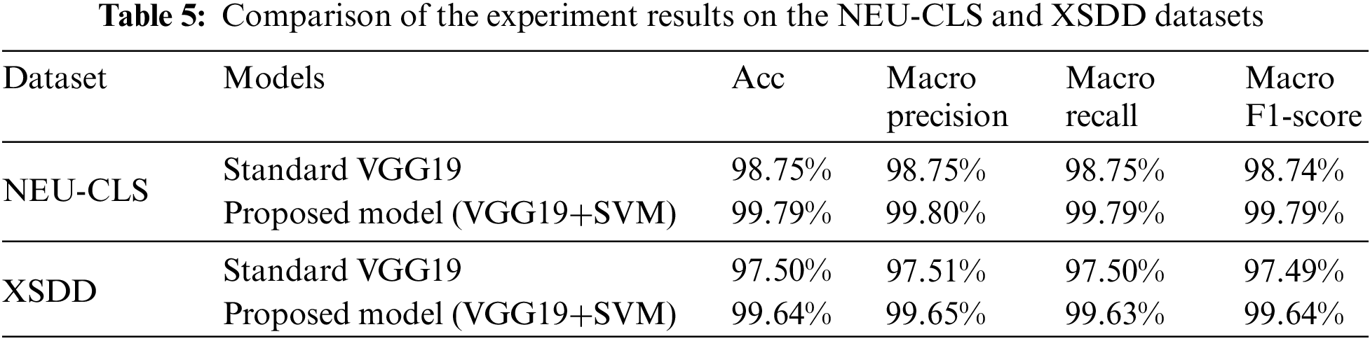
Table 5 shows a comparison of the experiment outcomes for the NEU-CLS and XSDD datasets. We chose standard VGG19 with Softmax classifier for comparison with our proposed model. Our proposed methodology outperforms the standard VGG19 models, showcasing superior results in terms of Accuracy, Precision, Recall, and F1-score. For the NEU-CLS dataset, our approach achieved high metrics, with 99.79% Accuracy, 99.80% Precision, 99.79% Recall, and 99.79% F1-score. In terms of Accuracy, Precision, Recall, and F1-score, these values outperform the standard VGG19 by 1.04%, 1.05%, 1.04%, and 1.05% points, respectively. For the XSDD dataset, our approach achieved high metrics, with 99.64% Accuracy, 99.65% Precision, 99.63% Recall, and 99.64% F1-score. In terms of accuracy, precision, recall, and F1-score, these values outperform the standard VGG19 by 2.14%, 2.14%, 2.13%, and 2.15% points, respectively, as shown in Table 5.

4.3 Experiment Results for NEU Dataset

In Fig. 9, we can see the confusion matrix for the standard VGG19 model. It provides insights into how VGG19 distinguishes between various defect types. Notably, this model exhibits misclassifications, with inclusion defect types having just one misclassified image as a pitted surface. For patch defect type, two images are misclassified, one as crazing and the other as a pitted surface. Similarly, pitted surface misclassifies two images, one as an inclusion and the other as patches. Scratches misclassify only one image as inclusion, while the model correctly classifies other defect types.

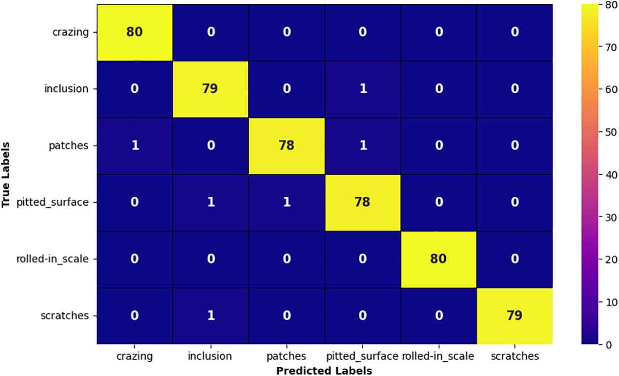
Figure 9: Confusion matrix of standard VGG19

Fig. 10 illustrates the confusion matrix of our proposed hybrid model. Fig. 10 displays how well our hybrid model correctly identifies different types of defects, except for one class where it mistakenly classifies a patch as a crazing. The reason behind this misclassification might be that the visual patterns of these two types of defects look quite similar, leading to confusion. Overall, the model performs exceptionally well in accurately identifying most types of defects.

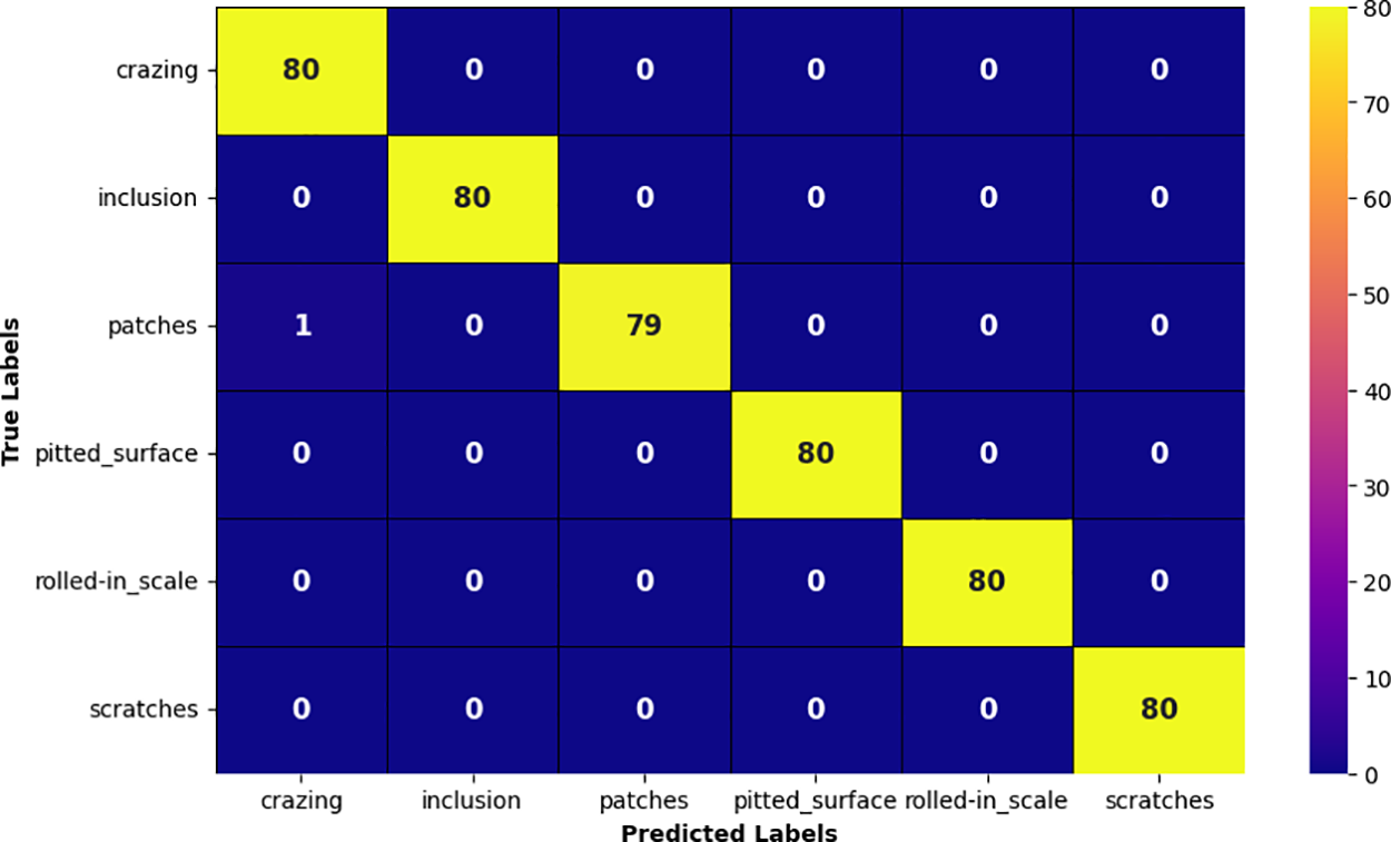
Figure 10: Confusion matrix of our proposed hybrid model

Fig. 11 provides a visual representation of how well our proposed model is doing in terms of accuracy and loss. In the first 10 iterations, we see a rapid improvement, with the loss decreasing quickly and accuracy increasing. As the learning rate decreases, the model starts to stabilize, and by the end of the iteration, the loss reaches close to zero.

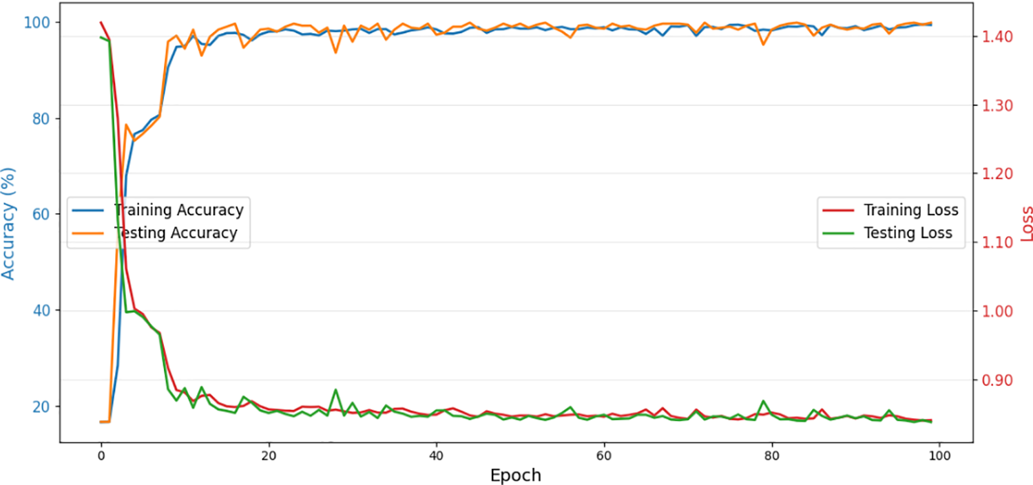
Figure 11: Accuracy and loss curves of the proposed model for the NEU dataset

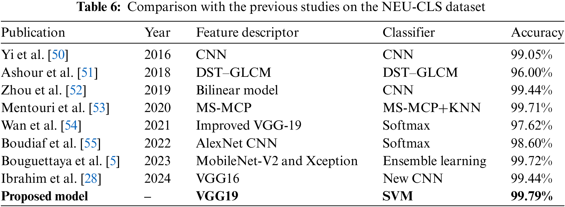
Table 6 presents a comparison with previous studies on the NEU-CLS dataset. The suggested hybrid system, which utilizes VGG19 as a feature extractor, GAP layer, and SVM classifier instead of Softmax, achieves high performance with 99.79% accuracy in the classification of different defect types of the NEU-CLS dataset. This remarkable outcome outperforms all other studies mentioned in Table 6, even those that used DL-based approaches. It shows the suggested system’s efficiency and excellence in accurately classifying steel defects when compared to existing techniques.

4.4 Experiments Results for the XSSD Dataset

In Fig. 12, we can see the confusion matrix for the standard VGG19 model. It provides insights into how VGG19 classified different defect types. Notably, this model shows misclassifications. For the finishing roll printing defect type, there is just one misclassified image, labeled as a red iron. Regarding the iron sheet ash defect type, one image is misclassified as finishing roll printing. In the case of the oxide scale plate system defect type, five images are misclassified, two as oxide scale temperature system, one as a red iron, and the other two as slag inclusion. For the red iron defect type, two images are misclassified, one as an oxide scale plate system and the other as an oxide scale temperature system. Moving to the slag inclusion defect type, four images are misclassified—one as an oxide scale temperature system, one as a red iron, one as an oxide scale plates system, and the remaining one as a surface scratch. As for surface scratches, only one image is misclassified as an oxide scale plate system. On the other hand, for the oxide scale temperature system defect type, all images are correctly classified with 100% accuracy.

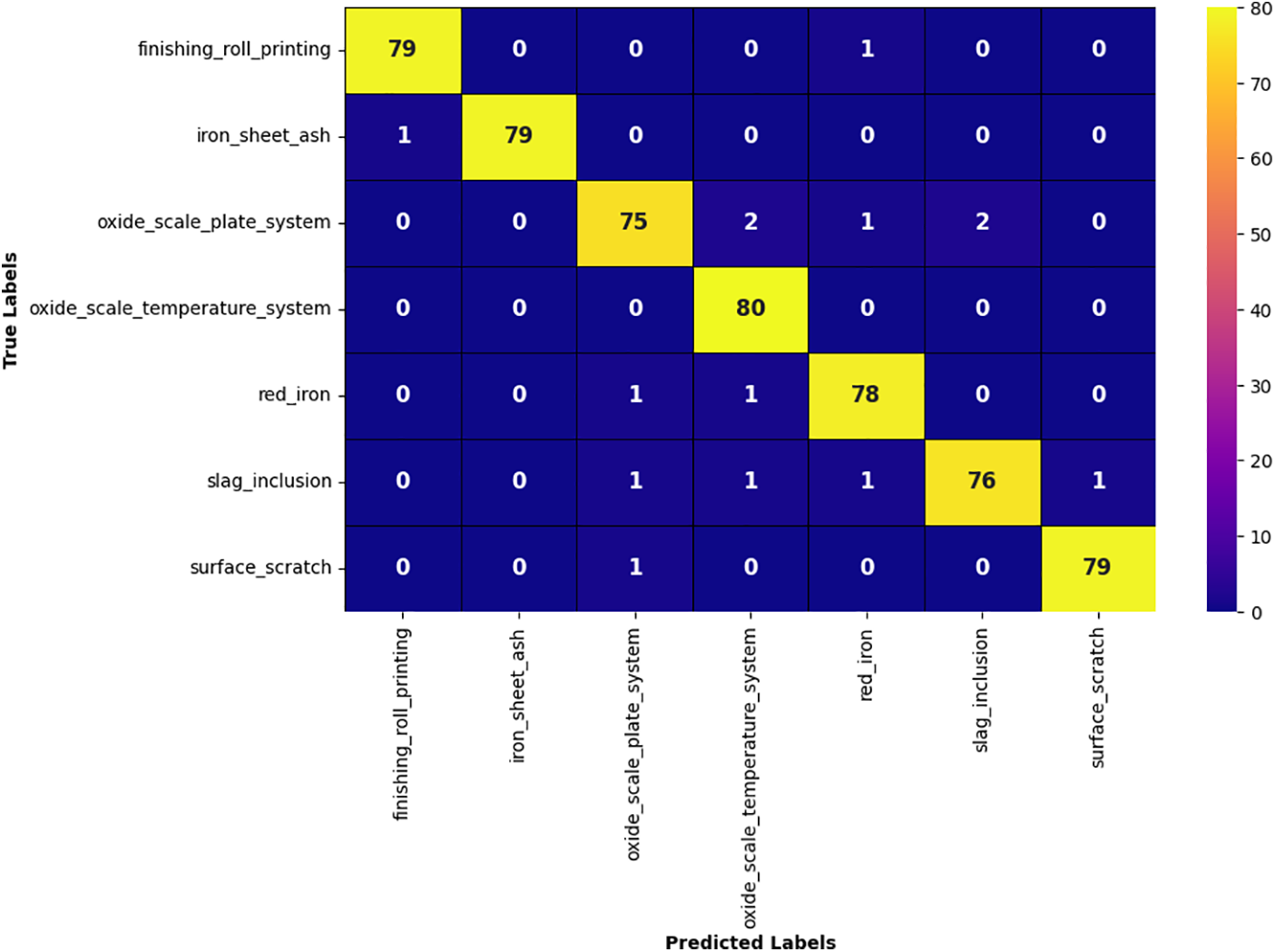
Figure 12: Confusion matrix of standard VGG19

Fig. 13 illustrates the confusion matrix of our proposed hybrid model. Fig. 13 displays how well our hybrid model can correctly classify different types of defects, except for one class where it mistakenly classifies two images of an oxide scale plate system one as an oxide scale temperature system and one as a surface scratch. On the other hand, for the other defect types, all images are correctly classified with 100% accuracy. The reason behind this misclassification might be that the visual patterns of these two types of defects look quite similar, leading to confusion. Overall, the model performs exceptionally well in accurately identifying all types of defects except one. Fig. 14 provides a visual representation of how well our proposed model is doing in terms of accuracy and loss. Our data shows that the recognition accuracy of our proposed hybrid model confirms its suitability for the task of classifying defects in a steel strip.

Figure 13: Confusion matrix of our proposed hybrid model

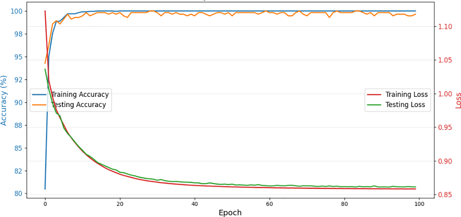
Figure 14: Accuracy and loss curves of the proposed model for the XSDD dataset

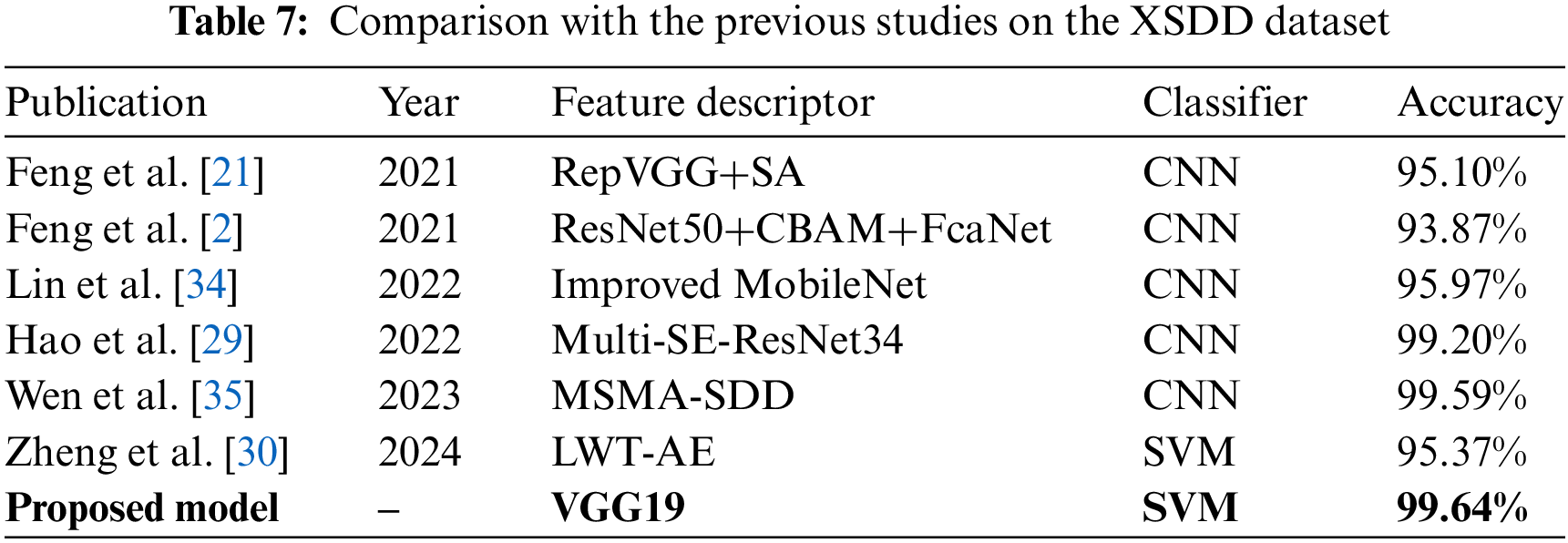
Table 7 presents a comparison with previous studies on the NEU-CLS dataset. The suggested hybrid system, which utilizes VGG19 as a feature extractor, GAP layer, and SVM classifier instead of Softmax, achieves high performance with 99.64% accuracy in the classification of different defect types of the XSDD dataset. This remarkable outcome outperforms all other studies mentioned in Table 7. It shows the suggested system’s efficiency and excellence in accurately classifying steel defects when compared to existing techniques.

5  Conclusion

This work suggests a hybrid model based on ML and DL for classifying defects in hot rolled steel strips. This approach utilizes a CNN model based on the VGG19 architecture with an SVM classifier and GAP layer, along with image processing and augmentation techniques, to address the challenges of accurately classifying surface defects on hot rolled steel strips. The issue of imbalanced and limited dataset is resolved by utilizing offline augmentation techniques. The experimental results show that VGG19 with Softmax classifier achieves an accuracy of 98.75% for the NEU-CLS dataset and 97.50% for the XSDD dataset, while the proposed methodology achieves the highest accuracy of 99.79% for the NEU-CLS dataset and 99.64% for the XSDD dataset. Our findings indicate that the SVM classifier outperforms the Softmax classifier in terms of accuracy, with a 1.04% improvement for the NEU-CLS dataset and a 2.14% improvement for the XSSD dataset. The success of our method can be attributed to the use of a powerful feature extractor and an SVM classifier. Our approach has shown an increase in accuracy as compared to other recent studies, as shown in Tables 6 and 7. Moreover, our future work will investigate the performance of hybrid networks with different combinations of backbone CNN architectures and classifiers.

Acknowledgement: The authors want to say thank you to the National Research Foundation of Korea (NRF) and the Ministry of Education for their financial support.

Funding Statement: This research was supported by the Basic Science Research Program through the National Research Foundation of Korea (NRF) funded by the Ministry of Education (NRF-2022R1I1A3063493).

Author Contributions: Study conception and design: Tajmal Hussain and Jongwon Seok; data collection: Tajmal Hussain and Jungpyo Hong; analysis and interpretation of results: Tajmal Hussain; draft manuscript preparation: Tajmal Hussain, Jungpyo Hong, and Jongwon Seok. All authors reviewed the results and approved the final version of the manuscript.

Availability of Data and Materials: The data are available from the corresponding author upon reasonable request.

Conflicts of Interest: The authors declare that they have no conflicts of interest to report regarding the present study.

References

1. W. P. Tang et al., “Design of multi-receptive field fusion-based network for surface defect inspection on hot-rolled steel strip using lightweight dataset,” Appl. Sci., vol. 11, no. 20, pp. 9473, Oct. 2021. doi: 10.3390/app11209473. [Google Scholar] [CrossRef]

2. X. Feng, X. Gao, and L. Luo, “A ResNet50-based method for classifying surface defects in hot-rolled strip steel,” Mathematics, vol. 9, no. 19, pp. 2359, Sep. 2021. doi: 10.3390/math9192359. [Google Scholar] [CrossRef]

3. A. Aldunin, “Development of method for calculation of structure parameters of hot-rolled steel strip for sheet stamping,” J. Chem. Technol. Metall., vol. 52, no. 1, pp. 737–740, Jan. 2017. [Google Scholar]

4. Z. W. Xu, X. M. Liu, and K. Zhang, “Mechanical properties prediction for hot rolled alloy steel using convolutional neural network,” IEEE Access, vol. 7, no. 1, pp. 47068–47078, Jan. 2019. doi: 10.1109/ACCESS.2019.2909586. [Google Scholar] [CrossRef]

5. A. Bouguettaya, Z. Mentouri, and H. Zarzour, “Deep ensemble transfer learning-based approach for classifying hot-rolled steel strips surface defects,” Int. J. Adv. Manuf. Technol., vol. 125, no. 11–12, pp. 5313–5322, Feb. 2023. doi: 10.1007/s00170-023-10947-8. [Google Scholar] [CrossRef]

6. Q. Luo, X. Fang, L. Liu, C. Yang, and Y. Sun, “Automated visual defect detection for flat steel surface: A survey,” IEEE Trans. Instrum. Meas., vol. 69, no. 3, pp. 626–644, Mar. 2020. doi: 10.1109/TIM.2019.2963555. [Google Scholar] [CrossRef]

7. N. Neogi, D. K. Mohanta, and P. K. Dutta, “Review of vision-based steel surface inspection systems,” EURASIP J. Image Video, vol. 2014, no. 1, pp. 1–19, Nov. 2014. doi: 10.1186/1687-5281-2014-50. [Google Scholar] [CrossRef]

8. J. Li, Z. Su, J. Geng, and Y. Yin, “Real-time detection of steel strip surface defects based on improved yolo detection network,” IFAC-PapersOnLine, vol. 51, no. 21, pp. 76–81, Aug. 2018. doi: 10.1016/j.ifacol.2018.09.412. [Google Scholar] [CrossRef]

9. A. Rehman, A. Paul, M. A. Yaqub, and M. M. U. Rathore, “Trustworthy intelligent industrial monitoring architecture for early event detection by exploiting social IoT,” in Proc. SAC’20, Brno, Czech Republic, 2020, pp. 2163–2169. [Google Scholar]

10. A. Jan and G. M. Khan, “Real world anomalous scene detection and classification using multilayer deep neural networks,” Int. J. Interact. Multimed. Artif. Intell., vol. 8, no. 2, pp. 158–167, Jun. 2023. doi: 10.9781/ijimai.2021.10.010. [Google Scholar] [CrossRef]

11. K. Song, J. Wang, Y. Bao, L. Huang, and Y. Yan, “A novel visible-depth-thermal image dataset of salient object detection for robotic visual perception,” IEEE/ASME Trans. Mechatron., vol. 28, no. 3, pp. 1558–1569, Jun. 2022. doi: 10.1109/TMECH.2022.3215909. [Google Scholar] [CrossRef]

12. K. Song and Y. Yan, “A noise robust method based on completed local binary patterns for hot-rolled steel strip surface defects,” Appl. Surf. Sci., vol. 285, no. 1, pp. 858–864, Nov. 2013. doi: 10.1016/j.apsusc.2013.09.002. [Google Scholar] [CrossRef]

13. Q. Luo et al., “Generalized completed local binary patterns for time-efficient steel surface defect classification,” IEEE Trans. Instrum. Meas., vol. 68, no. 3, pp. 667–679, Mar. 2018. doi: 10.1109/TIM.2018.2852918. [Google Scholar] [CrossRef]

14. S. Karthikeyan, M. Pravin, B. Sathyabama, and M. Mareeswari, “DWT based LCP features for the classification of steel surface defects in SEM images with KNN classifier,” Aust. J. Basic Appl. Sci., vol. 10, no. 5, pp. 13–19, Mar. 2016. [Google Scholar]

15. J. Zhang, X. Kang, H. Ni, and F. Ren, “Surface defect detection of steel strips based on classification priority YOLOv3-dense network,” IronmakSteelmak, vol. 48, no. 5, pp. 547–558, Sep. 2020. doi: 10.1080/03019233.2020.1816806. [Google Scholar] [CrossRef]

16. Y. J. Guo, Z. J. Sun, H. X. Sun, and X. L. Song, “Texture feature extraction of steel strip surface defect based on gray level co-occurrence matrix,” in Proc. ICMLC, Guangzhou, China, 2015, pp. 217–221. [Google Scholar]

17. H. Hu, Y. Liu, M. Liu, and L. Nie, “Surface defect classification in large-scale strip steel image collection via hybrid chromosome genetic algorithm,” Neurocomputing, vol. 181, no. 1, pp. 86–95, Mar. 2016. doi: 10.1016/j.neucom.2015.05.134. [Google Scholar] [CrossRef]

18. M. Jiang, G. Li, L. Xie, M. Xiao, and L. Yi, “Adaptive classifier for steel strip surface defects,” in Proc. CCISP, Dubai, United Arab Emirates, 2016, pp. 012019. [Google Scholar]

19. L. A. Martins, F. L. Pádua, and P. E. Almeida, “Automatic detection of surface defects on rolled steel using computer vision and artificial neural networks,” in Proc. IECON, Glendale, AZ, USA, 2010, pp. 1081–1086. [Google Scholar]

20. S. Y. Lee, B. A. Tama, S. J. Moon, and S. Lee, “Steel surface defect diagnostics using deep convolutional neural network and class activation map,” Appl. Sci., vol. 9, no. 24, pp. 5449, Dec. 2019. doi: 10.3390/app9245449. [Google Scholar] [CrossRef]

21. X. Feng, X. Gao, and L. Luo, “X-SDD: A new benchmark for hot rolled steel strip surface defects detection,” Symmetry, vol. 13, no. 4, pp. 706, Apr. 2021. doi: 10.3390/sym13040706. [Google Scholar] [CrossRef]

22. D. Chen, J. Wen, and C. Lv, “A spatio-temporal attention graph convolutional networks for sea surface temperature prediction,” Int. J. Interact. Multimed. Artif. Intell., vol. 8, no. 1, pp. 64–72, Feb. 2023. doi: 10.9781/ijimai.2023.02.011. [Google Scholar] [CrossRef]

23. A. Rehman, D. Kim, and A. Paul, “Convolutional neural network model for fire detection in real-time environment,” Comput. Mater. Contin., vol. 77, no. 2, pp. 2289–2307, Nov. 2023. doi: 10.32604/cmc.2023.036435. [Google Scholar] [CrossRef]

24. S. Iqbal, A. N. Qureshi, M. Alhussein, K. Aurangzeb, and M. S. Anwar, “AD-CAM: Enhancing interpretability of convolutional neural networks with a lightweight framework-from black box to glass box,” IEEE J. Biomed. Health. Inform., vol. 28, no. 1, Nov. 2023. doi: 10.1109/JBHI.2023.3329231. [Google Scholar] [PubMed] [CrossRef]

25. F. Wahab et al., “Design and implementation of real-time object detection system based on single-shoot detector and OpenCV,” Front. Psychol., vol. 13, no. 1, pp. 1039645, Nov. 2022. doi: 10.3389/fpsyg.2022.1039645. [Google Scholar] [PubMed] [CrossRef]

26. N. Kheradmandi and V. Mehranfar, “A critical review and comparative study on image segmentation-based techniques for pavement crack detection,” Constr. Build. Mater., vol. 321, no. 1, pp. 126162, Feb. 2022. doi: 10.1016/j.conbuildmat.2021.126162. [Google Scholar] [CrossRef]

27. S. Jain, G. Seth, A. Paruthi, U. Soni, and G. Kumar, “Synthetic data augmentation for surface defect detection and classification using deep learning,” J. Intell. Manuf., vol. 33, no. 1, pp. 1007–10220, Nov. 2022. doi: 10.1007/s10845-020-01710-x. [Google Scholar] [CrossRef]

28. A. A. M. Ibrahim and J. R. Tapamo, “Transfer learning-based approach using new convolutional neural network classifier for steel surface defects classification,” Sci. Afr., vol. 23, no. 1, pp. e02066, Mar. 2024. doi: 10.1016/j.sciaf.2024.e02066. [Google Scholar] [CrossRef]

29. Z. Hao, Z. Li, F. Ren, S. Lv, and H. Ni, “Strip steel surface defects classification based on generative adversarial network and attention mechanism,” Metals, vol. 12, no. 2, pp. 311, Feb. 2022. doi: 10.3390/met12020311. [Google Scholar] [CrossRef]

30. X. Zheng, W. Liu, and Y. Huang, “A novel feature extraction method based on legendre multi-wavelet transform and auto-encoder for steel surface defect classification,” IEEE Access, vol. 12, no. 1, pp. 5092–5102, Jan. 2024. doi: 10.1109/ACCESS.2024.3349628. [Google Scholar] [CrossRef]

31. D. Masko and P. Hensman, “The impact of imbalanced training data for convolutional neural networks,” M.S. thesis, KTH Royal Institute of Technology, Stockhom, Sweden, 2015. [Google Scholar]

32. Ö. E. Par, E. A. Sezer, and H. Sever, “Small and unbalanced data set problem in classification,” in Proc. SIU, Sivas, Turkey, 2019, pp. 1–4. [Google Scholar]

33. L. Xu, G. Tian, L. Zhang, and X. Zheng, “Research of surface defect detection method of hot rolled strip steel based on generative adversarial network,” in Proc. 2019 Chin. Automat. Congr., Hangzhou, China, 2019, pp. 401–404. [Google Scholar]

34. L. Lin et al., “Small samples data augmentation and improved MobileNet for surface defects classification of hot-rolled steel strips,” J. Electron. Imag., vol. 31, no. 6, pp. 063056, Nov. 2022. doi: 10.1117/1.JEI.31.6.063056. [Google Scholar] [CrossRef]

35. L. Wen, Y. Zhang, L. Gao, X. Li, and M. Li, “A new multi-scale multi-attention convolutional neural network for fine-grained surface defect detection,” IEEE Trans. Instrum. Meas., vol. 72, no. 1, pp. 1–11, Jan. 2023. doi: 10.1109/TIM.2023.3271743. [Google Scholar] [CrossRef]

36. C. Shorten and T. M. Khoshgoftaar, “A survey on image data augmentation for deep learning,” J. Big Data, vol. 6, no. 1, pp. 1–48, Jul. 2019. doi: 10.1186/s40537-019-0197-0. [Google Scholar] [CrossRef]

37. Y. Chen, Q. Fu, and G. Wang, “Surface defect detection of nonburr cylinder liner based on improved YOLOv4,” Mob. Inf. Syst., vol. 2021, no. 1, pp. 1–13, Jun. 2021. doi: 10.1155/2021/9374465. [Google Scholar] [CrossRef]

38. J. Zhang, G. Cosma, and J. Watkins, “Image enhanced mask R-CNN: A deep learning pipeline with new evaluation measures for wind turbine blade defect detection and classification,” J. Imag., vol. 7, no. 3, pp. 46, Mar. 2021. doi: 10.3390/jimaging7030046. [Google Scholar] [PubMed] [CrossRef]

39. Z. Q. Zhao, P. Zheng, S. T Xu, and X. Wu, “Object detection with deep learning: A review,” IEEE Trans. Neural. Netw. Learn. Syst., vol. 30, no. 11, pp. 3212–3232, Jan. 2019. doi: 10.1109/TNNLS.2018.2876865. [Google Scholar] [PubMed] [CrossRef]

40. L. Alzubaidi et al., “Review of deep learning: Concepts, CNN architectures, challenges, applications, future directions,” J. Big Data, vol. 8, no. 1, pp. 1–74, Mar. 2021. doi: 10.1186/s40537-021-00444-8. [Google Scholar] [PubMed] [CrossRef]

41. C. Tan et al., “A survey on deep transfer learning,” in Proc. Artif. Neural Netw. Mach. Learn., Rhodes, Greece, 2018, pp. 270–279. [Google Scholar]

42. O. Russakovsky et al., “ImageNet large scale visual recognition challenge,” Int. J. Comput. Vis., vol. 115, no. 3, pp. 211–252, Dec. 2015. doi: 10.1007/s11263-015-0816-y. [Google Scholar] [CrossRef]

43. K. Weiss, T. M. Khoshgoftaar, and D. Wang, “A survey of transfer learning,” J. Big Data, vol. 3, no. 1, pp. 1–40, May 2016. doi: 10.1186/s40537-016-0043-6. [Google Scholar] [CrossRef]

44. K. Simonyan and A. Zisserman, “Very deep convolutional networks for large-scale image recognition,” arXiv preprint arXiv:14091556, 2014. [Google Scholar]

45. Y. Tang, “Deep learning using linear support vector machines,” arXiv preprint arXiv:13060239, 2013. [Google Scholar]

46. A. F. Agarap, “An architecture combining convolutional neural network (CNN) and support vector machine (SVM) for image classification,” arXiv preprint arXiv:171203541, 2017. [Google Scholar]

47. M. Lin, Q. Chen, and S. Yan, “Network in network,” arXiv preprint arXiv:13124400, 2013. [Google Scholar]

48. V. Vapnik, “Support-vector networks,” Mach. Learn., vol. 20, no. 1, pp. 273–297, Sep. 1995. doi: 10.1007/BF00994018. [Google Scholar] [CrossRef]

49. S. S. Lad and A. C. Adamuthe, “Malware classification with improved convolutional neural network model,” Int. J. Comput. Netw. Inf. Secur., vol. 12, no. 6, pp. 30–43, Dec. 2020. doi: 10.5815/ijcnis.2020.06.03. [Google Scholar] [CrossRef]

50. L. Yi, G. Li, and M. Jiang, “An end-to-end steel strip surface defects recognition system based on convolutional neural networks,” Steel Res. Int., vol. 88, no. 2, pp. 1600068, Apr. 2016. doi: 10.1002/srin.201600068. [Google Scholar] [CrossRef]

51. M. W. Ashour, F. Khalid, A. Abdul Halin, L. N. Abdullah, and S. H. Darwish, “Surface defects classification of hot-rolled steel strips using multi-directional shearlet features,” Arab J. Sci. Eng., vol. 44, no. 1, pp. 2925–2932, Jun. 2019. doi: 10.1007/s13369-018-3329-5. [Google Scholar] [CrossRef]

52. F. Zhou, G. Liu, F. Xu, and H. Deng, “A generic automated surface defect detection based on a bilinear model,” Appl. Sci., vol. 9, no. 15, pp. 3159, Aug. 2019. doi: 10.3390/app9153159. [Google Scholar] [CrossRef]

53. Z. Mentouri, H. Doghmane, A. Moussaoui, and H. Bourouba, “Improved cross pattern approach for steel surface defect recognition,” Int. J. Adv. Manuf. Tech., vol. 110, no. 11–12, pp. 3091–3100, Sep. 2020. doi: 10.1007/s00170-020-06050-x. [Google Scholar] [CrossRef]

54. X. Wan, X. Zhang, and L. Liu, “An improved VGG19 transfer learning strip steel surface defect recognition deep neural network based on few samples and imbalanced datasets,” Appl. Sci., vol. 11, no. 6, pp. 2606, Mar. 2021. doi: 10.3390/app11062606. [Google Scholar] [CrossRef]

55. A. Boudiaf et al., “Automatic surface defect recognition for hot-rolled steel strip using AlexNet convolutional neural network,” in Int. Conf. Imag. Signal Process. their Appl., Mostaganem, Algeria, 2022, pp. 1–5. [Google Scholar]