Novel Fractal-Based Features for Low-Power Appliances in Non-Intrusive Load Monitoring

1  Introduction

Monitoring the electrical system at individual load levels often enables condition-based diagnostics and forecasts that can minimize the impact of equipment malfunctions or system failures [1]. Appliance-specific data empowers consumers to gain a better understanding of their energy consumption, resulting in informed decisions and rational energy use. This awareness, supported by appliance-specific feedback and potential load forecasting, can lead to tangible energy savings and environmental impact [2].

Nonintrusive Load Monitoring (NILM) is a low-cost solution to the load monitoring problem and it provides the necessary information in real-time to formulate various energy management schemes [3]. The NILM module consists of a single set of voltage and current sensors deployed at the main power entry point. Information extracted from the composite current and voltage signals is used for load disaggregation. While numerous techniques out there focus on high-power appliances, low-power appliance disaggregation is often overlooked. They are particularly difficult to disaggregate due to their nonlinearity and low power consumption. This research work attempts to solve the problem of low-power appliance disaggregation. and focuses on an event-based NILM approach. A novel feature extraction technique based on fractal analysis for the classification of low-power appliances is proposed.

Fractal analysis is a powerful technique that mathematically defines patterns in apparently random and complex figures [4]. Transients generated in electrical signals also exhibit fractal properties, but this technique has not yet been extensively used in power systems. The signal analysis domain is seeing quite a lot of fractal-related research, especially for medical diagnostics and wind turbine damage diagnostics [5,6]. Fractal techniques are not yet applied for feature extraction in NILM and will be done for the first time as part of this research.

The concept of NILM was first introduced by MIT researcher Hart in the 1980s [7]. It is an inexpensive tool for achieving energy disaggregation within a building without the expense of complicated hardware [8]. To classify or segregate the appliances, it is essential to first acquire and comprehend the features of the appliances. These features can capture several categories of appliance data, including patterns of turning on and off, voltage and current measurements, power consumption (actual, reactive, and apparent), and temporal fluctuations. There exist diverse categories of appliances, each possessing its unique power profile. Segregating two devices with significantly distinct power profiles is a straightforward procedure. However, if multiple appliances have power profiles that are roughly comparable, the process of segregation becomes challenging.

Earlier techniques of feature extraction focused on “steady-state” features like active and reactive powers and V-I trajectories [7,9–11]. The main advantage of using steady-state power is that it is easily and conveniently available. The main drawback of this approach is that it does not take into account the nonlinear loads. Considering the limitations of steady-state analysis, many researchers moved on to look for unique appliance signatures by analysing the transient state of loads. Electrical appliances demonstrate distinctive transient behaviour depending on their unique physical properties. Transient methods of analysis use different transformations to extract features from these transients and develop specific load/appliance signatures. For each appliance, a unique transient is generated when the appliance is switched ON/OFF [12]. This switching transient switching is more pronounced in the current signal. Initially, the Fourier transform was used to extract the transient feature [13]. Similarly, numerous studies based their feature extraction study on the harmonic analysis of switching transients [14,15]. The time-frequency analysis technique, wavelet transform and multiscale wavelet packet tree proved to be much more effective than traditional harmonic analysis methods [16–18].

Several hybrid and unconventional techniques also exist in the literature with a range of performance efficiencies [19–23]. The evolution of NILM techniques described above has been mostly tested on energy-intensive appliances. Additionally, the classification of devices that have extremely low power consumption is a challenge, as this minimal power level is typically considered as noise and they exhibit roughly similar profiles [10,24,25].

Based on the above literature review, there is still a void in the NILM research space for an effective feature extraction solution that works well with low-power appliance classification. Particularly, there is very little literature that deals with switching transient signals of low-power (less than 50 W) appliances with non-linear characteristics. The challenges include the difficulty in characterizing transient signals due to their short duration and wide frequency content. Existing methods such as spectrogram and wavelet decomposition have limitations in discriminating near similar transients. Additionally, the turn-on transient current of electrical appliances tends to decay to a steady state that is different from the one preceding it. To address these challenges, this research work has made the following research contributions:

1.    Mono- and Multi-Fractal Analysis is used for appliance classification in NILM research.

2.    The proposed fractal-based novel feature extraction method is compared with four other feature extraction methods, i.e., different variants of Scattering Transform and multi-level DWT.

3.    The proposed mono- and multi-fractal analysis method outshined all other feature extraction methods, achieving an accuracy of up to 96% with superior precision, recall, and F1-score values of up to 97.3%.

4.    Successfully used fractal analysis for low-power (less than 50 W) appliances.

The paper is organized as follows: Section 2 describes the mono- and multi-fractal methodology used to extract novel features from appliance switching current transients; Section 3 outlines the experimentation done including various test scenarios; Section 4 presents the result analysis and discussion and finally Section 5 concludes the paper.

2  Methodology

The selection of a suitable mathematical technique for time series analysis is based on its adaptability and practical applicability to real-world signals. Several real signals demonstrate nonlinear power-law characteristics, which are dependent upon higher-order moments and scale. In certain instances, the dynamic attributes of these processes exhibit multifractal as well as monofractal characteristics. This paper proposes to use the Wavelet Leaders Multifractal Formalism (WLMF) method, Higuchi’s method, and monofractal detrended fluctuation analysis (DFA) to extract multifractal and monofractal features of current switching transient for automatic classification of low-power electrical appliances.

2.1 Wavelet Leaders Multifractal Formalism

Fractal processes can be categorized into two types: Monofractal and multifractal [26]. A monofractal process is homogeneous, signifying uniform scaling properties that can be characterized by a single-scale indicator, such as fractal dimension or Hurst exponent, both locally and globally. In contrast, multifractal processes decompose into numerous homogeneous fractal subsets. The properties of these subsets can be characterized by a singularity spectrum and the Hölder exponents. This multifractal nature distinguishes them from mono-fractal processes. This paper proposes the adoption of both monofractal and multifractal features of current switching transients for the automatic classification of low-power appliances. Devices with extremely low power consumption pose a classification challenge, as this level of power is frequently misinterpreted as noise.

The Wavelet Leaders Multifractal Formalism (WLMF) method builds on wavelet coefficients obtained through the DWT following the Mallat pyramid scheme [27]. Subsequent stages of the algorithm include identifying coefficients known as wavelet leaders, calculating the structural function and scaling exponents, and determining the multifractal spectrum D(ℎ). Alternatively, the direct determination of spectrum parameters can be achieved using log cumulants.

Wavelet leaders are identified as space- or time-localized maxima of discrete wavelet coefficients. To achieve time localization of the maxima, it is necessary to derive the wavelet coefficients utilising a compactly supported wavelet. The Hölder exponents, which quantify the local regularity, are computed from these maxima. The size of the set of Hölder exponents in the time series is referred to as the singularity spectrum. Wavelet leaders are defined at any given scale as [27]:

Lx(j,k)=supλ′∈3λj,k|dx(j,k)|(1)

where the time neighbourhood 3λj,k=λj,k−1∪λj,k∪λj,k+1 and λj,k=[k2j,(k+1)2j] and dx(j,k) are the wavelet coefficients. The wavelet leaders serve as representatives of the Hölder exponents h: Lx(j,k)∼2jh.

The multi-resolution structure-function ZL(q,a) is defined as a spatial average of the q-th order of the leaders, given as:

ZL(q,a)=1na∑k=1na|Tx(a,k)|q≃aζ(q),(2)

where a represents the scale, q signifies the moment, Tx denotes the wavelet leaders by scale, na is the number of wavelet leaders at every scale, and ζ(q) represents the scaling exponent. The result of expanding ζ(q) to a polynomial is:

ζ(q)=c1q+c2q2/2+c3q3/6+…(3)

The scaling exponent ζ(q) of the structure function’s Legendre transform serves as an upper limit for the multifractal spectrum. Understanding the scaling exponent ζ(q) enables a direct estimation of parameters for the multifractal spectrum D(h) using log-cumulants cp with orders p≥1, derived from a Taylor series expansion. The signal is considered monofractal when ζ(q) is a linear function. A multifractal signal does not follow a linear pattern. In terms of scaling exponents, the first cumulant, c1, represents linear behaviour, while the second and third cumulants, c2 and c3, respectively, denote non-linearity. The multifractal spectrum D(h), derived by the Legendre transform of the scaling exponents, where h is the Hölder exponent is given as:

D(h)=infq≠0(1+qh−ζ(q)).(4)

2.2 Hurst Exponent Computation

The monofractal structure of a time series is characterized by the Hurst exponent HE, which determines the rate at which the overall root-mean-square (RMS) of local fluctuations increases with a growing segment sample size or scale. In detrended fluctuation analysis (DFA), the RMS fluctuation is calculated for various segment sizes, and the scaling behaviour is expressed as a power-law relation [28]. The exponent of this power-law relation is referred to as the Hurst exponent. It is a measure of the long-range correlations or self-similarity in the time series.

Let Xt be the cumulative sum of a time series x1,x2,x3,…,xN:

Xt=∑i=1t(x1−⟨x⟩)(5)

Next, create an approximate geometric progression A={a1,a2,a3,…,ak}, such that, a1≈4, ak≈N, and a1<a2<a3<…<ak. Also, log⁡a2−log⁡a1≈log⁡a3−log⁡a2≈…. Split the sequence Xt into subsequent segments of length a for each ‘a’ belonging to A. Calculate the regression (the local trend) within each section. Considering Y1,a,Y2,a,Y3,a,…,YN,a as the resultant piecewise-linear approximation, the total fluctuation is the root mean square of the local fluctuation:

FT(a)=1N/a∑i=1NaFL(a,i)2(6)

where FL is given as:

FL(a,i)=1a∑t=ia+1ia+a(Xt−Yt,a)2(7)

The value of HE then could be estimated from the slope of the regression line:

log⁡(FT(a))=log⁡(C)+HE⋅log⁡(a)(8)

A Hurst exponent HE above 1 visually corresponds to slower-evolving variations, indicating a more persistent structure in monofractal and multifractal time series [28]. A signal exhibits a long-range dependent (correlated) structure when the Hurst exponent falls within the interval of 0.5–1, and it demonstrates an anti-correlated structure when the Hurst exponent is within the range of 0–0.5. In the special case where the Hurst exponent is equal to 0.5, the time series exhibits an independent or short-range dependent structure.

2.3 Higuchi’s Fractal Dimension Computation

Higuchi’s technique is used to estimate the fractal dimension of the start-up transient in the current waveform [29]. The values of the appliance current can be taken as a time series i(1),i(2),…,i(N). A new time series is constructed as follows:

imk={i(m),i(m+k),i(m+2k),…,x(m+[N−mk].k)}(9)

for m=1,2,…,k; where m is the initial time and k is the time interval. The total data points of the series are represented by N. Therefore, k set of new current series is constructed. The average length of each new time series is calculated as:

Bm(k)=1k[(∑a=1int[N−mk]|i(m+ak)−i(m+(a−1)k|)Xnorm](10)

Xnorm=N−1int[N−mk].k(11)

The total average length of k series, B(k), is then calculated as:

B(k)=1k[∑m=1kBm(k)](12)

If the series under consideration exhibits non-linear behaviour and has fractal-like properties, then:

B(k)∝k−FD(13)

where FD is the fractal dimension of the curve formed by the time series of the appliance current. Taking logarithms on both sides, the following is obtained:

ln⁡(B(k))∝FD.ln⁡(1/k)(14)

Graph of ln⁡(B(k)) is plotted against ln⁡(1k) for k=1,2,…,kmax and the least squares method is used to fit a straight line through the points. The slope of the fitted line FD is the fractal dimension of the time series.

2.4 Mono- and Multi-Fractal Features Extraction

This paper proposes to extract fractal dimension FD, Hurst exponent HE, multifractal spectrum D(h) and the Hölder exponents h of current switching transient signals. The total number of extracted features is 24. To exemplify the capability of fractal analysis in elucidating signal structures that may not be captured through traditional signal processing methodologies, the switching transients’ signals of a Charger and a Compact Fluorescent Lamp (CFL) are specifically chosen, as depicted in Fig. 1a. The signals’ second-order statistics are considerably comparable. Charger has a mean of 3.49e-4, a variance of 3.20e-4, and an RMS value of 0.02 and CFL has a mean of 3.05e-4, a variance of 7.30e-5, and an RMS value of 0.01, the values are almost identical.

Figure 1: (a) Current transient signals (b) PSD of signals (c) Multifractal spectrum and (d) Scaling exponents

The power spectral density (PSD) estimates shown in Fig. 1b are also very similar. The power spectrum provides information about the distribution of power across different frequencies in a signal. The Welch PSD estimate is an improvement over the standard periodogram method, addressing some of its limitations, particularly the variability in the spectral estimates. It divides the signal into overlapping segments, computes the periodogram for each segment, and then averages the resulting periodograms to obtain a smoother and more reliable estimate of the power spectrum. Fractal analysis reveals the substantial dissimilarity between these signals. The WLMF-based multifractal spectrum for both signals is presented in Fig. 1c. This multifractal spectrum illustrates the distribution of scaling exponents within a signal. The x-axis represents the range of Hölder exponents, which indicate the local scaling properties of the system. The y-axis represents the multifractal spectrum D(h), indicating the distribution of these local Hölder exponents. Examining the multifractal spectra in this context, the CFL signal exhibits a cluster of Hölder exponents centred around 0.2. In contrast, the charger signal showcases a cluster of Hölder exponents around 1.

Hölder exponents classify singularity strength by indicating their degree of differentiability. A Holder exponent equal to or less than 0 signifies a discontinuity at that specific location. Conversely, Holder exponents equal to or greater than 1 indicate differentiability at those locations. Holder values falling between 0 and 1 signify continuity but not differentiability at specific locations, revealing how closely the signal at that sample approaches differentiability. Holder exponents nearing 0 points to signal locations with lower differentiability compared to those with exponents closer to 1, suggesting a smoother signal at locations featuring higher local Holder exponents.

In Fig. 1d, the scaling exponents for both the charger and CFL signals are examined. Scaling exponents characterize how the statistical moments of a signal change with scale. For the positive and negative 1st-order statistical moments, the scaling exponents exhibit a linear relationship. This linearity suggests monofractality in the current signals for these specific moments. However, when considering moments from the 2nd order onwards, the scaling exponents deviate from linearity. This departure is likened to the behaviour of a multifractal process, which is characterized by a nonlinear scaling law. This observation suggests that the switching transient signals from the charger and CFL exhibit both monofractal and multifractal features. Therefore, this characteristic of mono- and multi-fractality in the transient signals is explored by extracting FD, HE, D(h), and h features in this research work.

3  Experimentation

3.1 Data Pre-Processing

This study employs the WHITED dataset as its primary data source. This dataset offers individual appliance current and voltage information for 5 s concurrently measured at a sampling rate of 44.1 kHz across eight distinct zones and under three distinct power supply standards [30]. To capture the switching transient signals of each appliance effectively, a meticulous pre-processing of the data is conducted. Given the research focus on the classification of low-power level devices, 10 appliances with variable instances are selected, resulting in a dataset comprising 250 signal instances, each comprising 1800 datapoints, as outlined in Table 1. The selection criteria for these 10 types involve ensuring that their power consumption remains below 50 W.

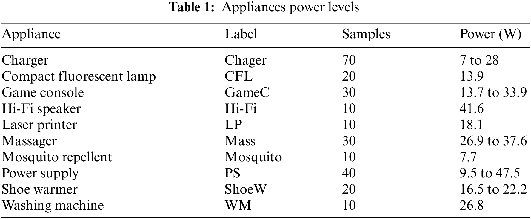
Fig. 2 illustrates the overall architecture of our proposed mono- and multi-fractal analysis-based feature extracted method.

Figure 2: Proposed low power appliances classification methodology

For each switching current transient of low-power devices in the WHITED dataset, the current transient is pre-processed, FD, HE, D(h), and h fractal features are extracted, four classifiers are optimized using Bayesian optimization, and precision, recall, F1-score, and accuracy performance metrics are used to test the performance of classification.

3.2 Simulation Scenarios and Performance Metrics for Comparison

To assess the efficacy of the proposed feature extraction methodology, the study conducts a series of comprehensive comparative experiments. Different strategies are employed to select features derived from Scattering Transform, multi-level DWT, and the proposed feature extraction method for low-power NILM signals. The features matrix is determined through five distinct strategies, outlined briefly below:

Scenario 1: considered both the first and second-order-path Scattering coefficients;

Scenario 2: considered only the first order-path Scattering coefficients;

Scenario 3: considered only the second order-path Scattering coefficients;

Scenario 4: considered the percentages of energies corresponding to the details of 5-level wavelet decomposition using the order 1 Daubechies wavelet.

Scenario 5: considered the proposed mono- and multi-fractal analysis features, i.e., fractal dimension FD, Hurst exponent HE, multifractal spectrum D(h) and the Hölder exponents h.

The performance of all five strategies is assessed using the commonly employed evaluation indices: Precision, recall, Fp-score, and accuracy. They are computed as follows:

Precision=TPFP+TP(15)

Recall=TPFN+TP(16)

Fp-score=(p2+1)∗(precision∗recall)p2∗(precision+recall)(17)

Accuracy=TP+TNTP+TN+FP+FN(18)

where TP represents true positives (the ON state of the appliance accurately predicted); FP represents false positives (actual state: ON; predicted state OFF); FN represents false negatives (actual state: OFF; predicted state ON) and TN (the OFF state of appliance accurately predicted); Furthermore, the harmonic parameter denoted as p is set to 1. These performance metrics pertain to individual appliances. The precision and recall indicators for all classification methods are calculated as the average of the indexes of the appliances. Furthermore, for imbalanced datasets, the Area Under the Curve (AUC) of the Receiver Operating Characteristic curve (ROC) can be a more reliable performance measure compared to accuracy alone. Therefore, we additionally analyzed the AUC to compare our classification models. The Receiver Operating Characteristic (ROC) is a visual representation of the relationship between the true positive rate and the false positive rate at different threshold values of the algorithm used for classification. The value of AUC can vary from 0 to 1, with a value of 1.0 representing flawless classification and a value below 0.5 indicating quasi-random guessing [31].

4  Results and Discussion

The performance of the proposed method (scenario 5) is tested using four optimized classifiers, i.e., deep neural network (DNN), SVM, decision trees, and KNN. Fig. 3 shows the progress of training for all the classifiers using the proposed feature extraction method until 30 iterations. In each case, all the classifiers are optimized using Bayesian optimization. Min classification error is used to optimize the hyperparameters of all the classifiers. The ‘min-observed’ classification criterion selects the best point hyperparameters. For the KNN classifier, the minimum observed error is 0.139 and the best point hyperparameters are achieved from the 9th iteration. For Decision Trees, the minimum observed error is 0.179 and the best point hyperparameters are achieved from the 11th iteration. Similarly, the minimum observed error for the SVM classifier is 0.128 and the best point hyperparameters are achieved from the 18th iteration. For the last DNN classifier, the minimum observed error is 0.125 and the best point hyperparameters are achieved from the 15th iteration.

Figure 3: Training progress of all classifiers when optimized using Bayesian optimization

The results of the Bayesian optimization with the proposed feature extraction method are shown in Table 2. The optimization technique targeted crucial classifier hyperparameters to thoroughly test the feature extraction method’s performance under different configurations. For the DNN, the optimization focused on the number of layers, regularization strength, activation function, and the number of neurons in each layer. The regularization strength parameter governs the impact of regularization on DNN. Larger values of regularization strength enforce more substantial penalties on large weights, deterring the model from excessive complexity and alleviating overfitting [32]. Striking the right balance is crucial, as excessive regularization may lead to underfitting, while insufficient regularization can result in overfitting. The non-linear activation function allows the learning of complex patterns. The resulting configuration comprised a network with three layers, a regularization strength of 5.96e-6, and specific neuron counts for each layer (9, 147, and 14 neurons in the first, second, and third layers, respectively). The computationally efficient Rectified Linear Unit (ReLU) activation function solves the vanishing gradient problem observed in sigmoid and tanh activation functions. It sets negative input values to zero, which promotes sparsity and helps the model learn faster and more effectively [33].

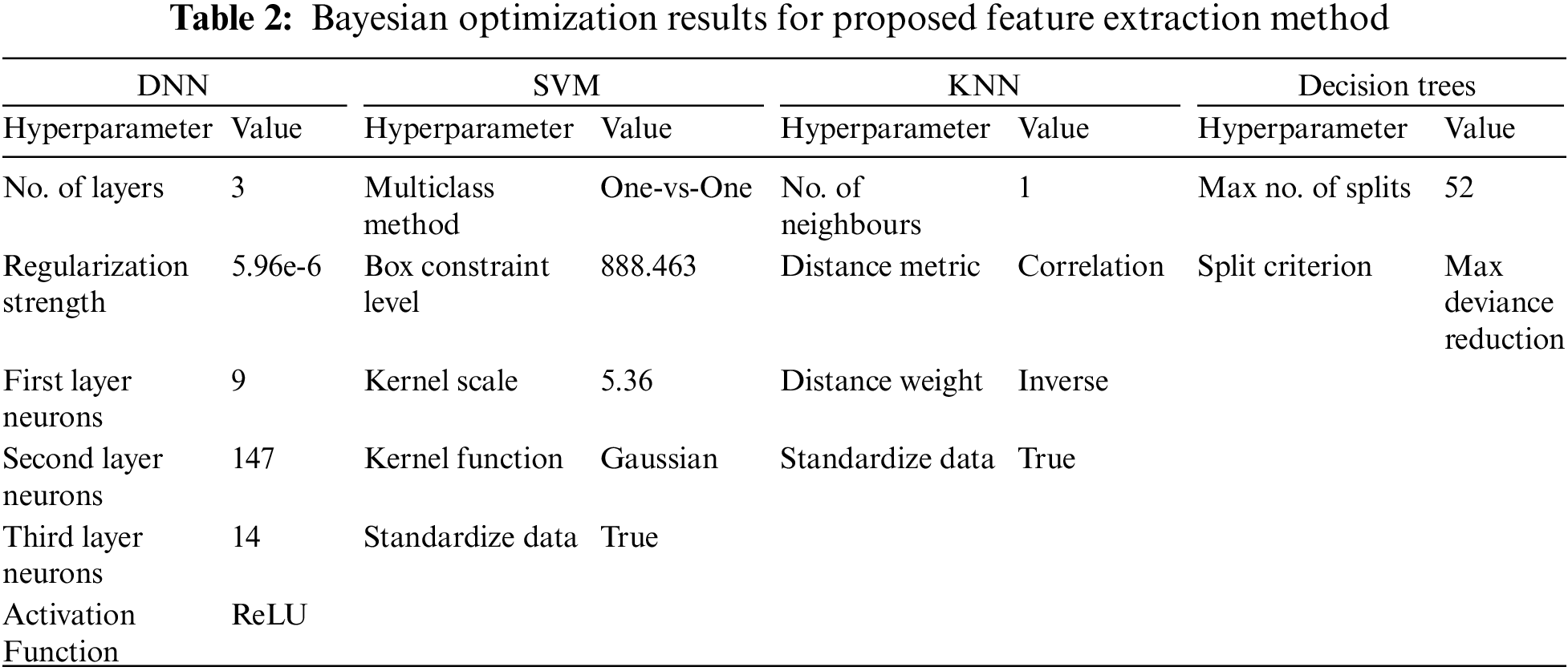
The SVM optimization model focuses on optimizing the multiclass technique, box constraint level, kernel scale, and kernel function. The selection of a multiclass technique is crucial in deciding its strategy for dealing with classification problems that involve more than two classes. The box constraint parameter plays a crucial role in striking a balance between accurately classifying training points and achieving a smooth decision boundary. The kernel scale parameter assumes significance in shaping the decision boundary by dictating the extent of influence wielded by each data point. Manipulating the kernel scale introduces variations in the boundary’s flexibility. The optimized configuration consists of a one-vs-one multiclass method, a box constraint level of 888.463, a kernel scale of 5.36, and a Gaussian kernel function. In one-vs-one, each class is treated as a binary classification problem against the rest. Additionally, data standardization was deemed beneficial for this SVM setup.

The KNN classifier was optimized by adjusting the number of neighbours, selecting an appropriate distance metric, and assigning weights to the distances. The number of neighbours indicates the degree to which nearby data points have an impact on the classification of a given point. The distance metric is used to calculate the distance between data points in the KNN algorithm, which determines the level of similarity or dissimilarity. In addition, the distance weight assigns different weights to surrounding points based on their distance from the query point. The complexity of this situation is essential in controlling the importance of each neighbour’s input in determining the final classification result. The optimized configuration dictated one neighbour, a correlation-based distance metric, and inverse distance weighting.

In the case of Decision Trees, the optimization targeted the maximum number of splits and the split criterion. This maximum number of splits establishes an upper limit on the depth of the decision tree. By limiting the maximum number of splits, the algorithm avoids creating an excessively deep tree, which could lead to overfitting the training data

Moreover, the split criterion determines the metric used to evaluate the quality of a split at each node. The resulting configuration included a maximum of 52 splits and the use of the “Max Deviance Reduction” criterion. Standardization of data was identified as advantageous for this Decision Trees setup. Table 3 shows the precision, recall, and F1-score of all the electrical appliances for all the optimized classifiers using the proposed feature extraction method.

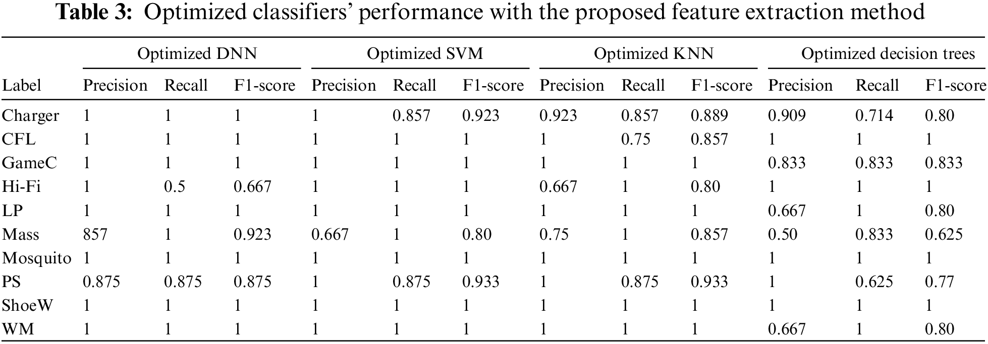
Furthermore, Figs. 4a–4c demonstrate bar charts of precision, recall, and F1-score of all the optimized classifier using the features extracted from the proposed multi- and mono-fractal analysis method. The DNN classifier demonstrated exceptional performance, achieving good scores for precision, recall, and F1-score for all appliances. For example, the Charger exhibited precision, recall, and F1-score values of 1, indicative of ideal classification accuracy.

Figure 4: (a) Precision, (b) recall, and (c) F1-score using the proposed feature extraction method for various classifiers

The SVM classifier also exhibited robust classification capabilities, yielding high precision and recall for most appliances. Similarly, the KNN classifier performed commendably, demonstrating good precision, recall, and F1-score values for various appliances The Decision Trees classifier also displayed reliable performance, with consistently high scores in precision, recall, and F1-score for multiple appliances. Nevertheless, appliances such as the Hi-Fi Speaker System and Massager exhibited slightly lower F1-scores, indicating potential areas for further optimization using advanced optimization techniques [34–36] or alternative classifier selection.

To provide a more holistic view, we complemented accuracy, F1-score, precision, and recall with the AUC metric. The value of AUC can vary from 0 to 1, with a value of 1.0 representing flawless classification and a value below 0.5 indicating quasi-random guessing. Table 4 gives the AUC values of various appliances for each optimized classifier. It is evident from the results that the DNN model and SVM have the highest overall performance with average AUC of 0.99 and 1.0, respectively. Then come the decision tree and KNN classification models with average AUC of 0.95 and 0.96, respectively. DNN, SVM, and KNN all achieved perfect AUC scores of 1 for several categories of appliances, indicating their ability to perfectly distinguish between classes in those cases. Overall, the performance of all the models was strong, with AUCs consistently surpassing 0.9 for the majority of appliances. This indicates that all of them possess a strong capacity to differentiate between the various categories of appliances. However, there were specific exceptions such as KNN for CFL with an AUC of 0.875, which is still considered good but lower than the others. Similarly, the decision tree for PS with an AUC of 0.7946, which is closer to the quasi-random guessing indicator of AUC = 0.5.

Considering all the discussed performance metrics, DNN was found to be the model that achieved the best classification results. These variations in performance metrics across classifiers underscore the importance of considering the specific characteristics of each appliance when choosing an optimal classifier.

4.1 Comparison with State-of-the-Art Methods

Table 5 compares the proposed multi- and mono-fractal-based feature extraction method with four other feature extraction methods described in sub-section 3.2 based on accuracy, precision, recall, and F1-score. All the feature extraction methods were tested using the same data. The performance has been compared for every optimized classifier, i.e., DNN, SVM, Decision Trees, KNN. Notably, the proposed mono- and multi-fractal analysis method outshines all other feature extraction methods.

Using the optimized DNN classifier, the method employing ST coefficients of all orders achieves an accuracy of 82% with similar levels of precision, recall, and F1-score. The approach focusing solely on first-order ST coefficients demonstrates an improved accuracy at 88%, showing improvement in capturing primary signal characteristics. However, the method considering second-order ST coefficients experiences a decrease in accuracy to 70%, indicating challenges in capturing more complex patterns.

The multi-level DWT method attains an accuracy of 84%, offering a balanced trade-off between precision and recall. Notably, the proposed mono- and multi-fractal analysis method outshines all other feature extraction methods, achieving an impressive accuracy of 96% with superior precision, recall, and F1-score values of 97.3%, 93.75%, and 95.5%, respectively.

Moving to the Support Vector Machine (SVM) classifier, the feature extraction methods display consistent performance across various metrics. The ST coefficients of all orders method achieves a low accuracy of 80%, with low precision, recall, and F1-score values. The ST coefficients of the first order show a slight increase in accuracy to 82% but lower values of precision, recall, and F1-score. Similarly, the second-order ST coefficients method records an even lower accuracy of 76% and similar smaller values of other performance metrics. The multi-level DWT method attains an accuracy of 78%, displaying a balanced performance. Once again, the proposed multi-fractal analysis method stands out, achieving a remarkable accuracy of 94%, emphasizing its effectiveness in optimizing SVM classification.

Different feature extraction approaches demonstrate varied performances for the Decision Trees classifier. The approach using ST coefficients of all orders as features produces a relatively low accuracy of 82% while maintaining a balanced performance in terms of precision, recall, and F1-score. The approach that uses only first-order ST coefficients achieves a marginally lower accuracy rate of 76% and considerably low precision and recall. The approach using second-order ST coefficients demonstrates a precision of 70%, suggesting difficulties in capturing intricate patterns. The Multi-level DWT approach produces a 72% accuracy and very low precision and recall values. The suggested multi-fractal analysis method once again demonstrates exceptional performance, obtaining an accuracy of 82% along with high precision, recall, and F1-score values, i.e., 85.76%, 90.05%, and 87.85%, respectively.

Lastly, in the evaluation of the KNN classifier, the feature extraction methods demonstrate robust performances. The ST coefficients of all orders achieves an accuracy of 92%, maintaining a balance between precision, recall, and F1-score. The first-order ST coefficients method maintains consistent accuracy at 92%, with balanced precision and recall. The second-order ST coefficients method records an accuracy of 82%, showcasing a solid performance. The multi-level DWT method attains a low accuracy level of 80% with poor precision, recall, and F1-score values. The proposed multi-fractal analysis method once again stands out, achieving an accuracy of 92%, precision of 93.4%, recall of 94.82%, and F1-score of 94.10, emphasizing its effectiveness in enhancing KNN classification accuracy.

4.2 Discussion

The coefficients in scattering transform (ST) in the first three scenarios are determined analytically and do not need to be learned. The ST also has time-shifting and small time-warping invariance, reducing the need for precise temporal localization for classification. It has shown promising results for classifying high-power level appliances such as vacuum cleaners [37] but its performance for low-power level appliances is seldom studied. Furthermore, it may not perform well in scenarios with small training datasets or limited labelled examples. Similarly, the 5-level DWT method of scenario 4 is seldom studied for low-power level appliances. The fifth scenario employs the proposed advanced fractal analysis techniques for feature extraction.

In the proposed hybrid mono- and multi-fractal analysis method, the fractal dimension captures the complexity of the signal, the Hurst exponent characterizes long-term dependencies, the multifractal spectrum describes the distribution of singularities, and the Hölder exponents provide information about local regularities. The hybrid approach integrated both mono- and multi-fractal features to optimize classification accuracy. When employing only mono-fractal features, specifically the Hurst exponent and Fractal dimension, the accuracy achieved was 64%. Similarly, employing only multi-fractal analysis resulted in an accuracy of 84%. However, the combination of these features proved highly effective with an accuracy of up to 96%. The synergistic combination of mono- and multi-fractal features evidently enhanced the overall classification performance, showcasing the robustness of the hybrid method in achieving superior accuracy compared to individual feature sets.

In general, the suggested method exhibited exceptional efficacy in categorizing low-power level appliances, a task that is frequently problematic for alternative algorithms that may erroneously classify such signals as background noise. It can manage the intricacy and lack of linearity that is inherent in low-power appliance signatures. The versatility of fractal-based techniques in handling signals with different levels of complexity enables an efficient differentiation between noise and real appliance patterns in the low-power range. It is intrinsically well-suited to deal with the lack of density in signals, emphasizing important features and enabling the reduction of dimensions. This is especially beneficial in situations with weak signals, as extraneous data might obscure the real characteristics of the devices. The utilization of a hierarchical representation provided by fractal analysis enhances the effectiveness of the procedure. On the contrary, other methods, such as ST coefficients or multi-level DWT have struggled to adapt to the intricacies of low-power appliance signals. Their representations have failed to adequately distinguish between noise and genuine appliance signatures in the low-power range.

For the comparative assessment of computational efficiency, the performance of the proposed multi-fractal and mono-fractal analysis methods is evaluated against established state-of-the-art techniques as shown in Table 6. The total execution time for the proposed multi-fractal analysis amounted to 1.364 s, featuring a minimal self-time of 0.008 s, with the predominant computational load attributed to child functions time, specifically 1.36 s. Conversely, the proposed mono-fractal analysis demonstrated a total execution time of 3.456 s, with a noteworthy self-time of 1.442 s, implying a substantial portion of the algorithm’s execution dedicated to internal computations. In comparison to the proposed methods, the multi-level DWT and ST analysis of all orders exhibited considerably higher total execution times of 153.84 and 81.41 s, respectively.

The multi-level DWT predominantly consumed time within the algorithm itself (153.04 s), while ST analysis distributed its computational load more evenly between self-time (1.165 s) and child functions’ time (80.25 s). This analysis underscores the efficiency of the proposed multi- and mono-fractal analysis, particularly in optimizing child functions time, highlighting its potential as a competitive alternative to existing methodologies.

Furthermore, the WHITED dataset contains appliance data from various regions across the world. For instance, the start-up transients of the charger are collected from three different regions of the world. The performance of the proposed algorithms suggests that fractal analysis can capture unique features from start-up transients of low-power nonlinear appliances regardless of their underlying circuit connection with the power mains. However, isolation of the switching transients plays an important role in the implementation of this methodology and event detection is very critical as this step directly determines the upper limit of the identification performance. Furthermore, this method needs to be tested for multi-switching of appliances and that is to be included as part of future work of this project.

5  Conclusion

This research work addresses a significant gap in NILM research by proposing a novel hybrid feature extraction method based on mono-fractal and multi-fractal approaches. While prior studies have focused on high-power appliances, our work specifically targets the challenging domain of low-power appliances, where distinguishing between devices with similar power profiles poses a considerable obstacle. The utilization of fractal dimension, Hurst exponent, multifractal spectrum, and Hölder exponents in the analysis of switching current transient signals has proven to be a robust approach, achieving superior performance compared to state-of-the-art methods. The comprehensive evaluation using precision, recall, F1-score, and accuracy consistently demonstrates the superiority of our mono- and multi-fractal analysis, achieving an outstanding accuracy of up to 96%.

This work not only advances the understanding of low-power appliance identification but also introduces a valuable methodology for feature extraction in NILM research. The successful application of fractal analysis in this context enhances the accuracy and efficiency of NILM, paving the way for more effective energy management strategies and increased awareness among consumers. These findings underscore the potential of fractal-based approaches in improving the performance of appliance recognition algorithms.

For future work, we plan to test this algorithm on aggregated measurements and develop a complete NILM solution that fuses various methods of appliance signature development to encompass low and medium-power appliances as well as energy-intensive appliances.

Acknowledgement: The authors are grateful to the University of Engineering and Technology Lahore for providing a platform to conduct this research.

Funding Statement: The authors received no specific funding for this study except from the regular research fund of the university.

Author Contributions: Anam Mughees: Conceptualization, Methodology, Software, Data curation, Validation, Writing-original draft preparation, Formal analysis. Muhammad Kamran: Conceptualization, Formal analysis, Supervision, Project administration, Validation.

Availability of Data and Materials: Data is openly available in a public repository. The data that support the findings of this study are openly available at https://www.cs.cit.tum.de/dis/resources/whited/.

Conflicts of Interest: The authors declare that they have no conflicts of interest to report regarding the present study.

References

1. H. Malik, A. Iqbal, and A. K. Yadav, Soft Computing in Condition Monitoring and Diagnostics of Electrical and Mechanical Systems. Singapore: Springer, 2020. vol. 1096. [Google Scholar]

2. G. F. Angelis, C. Timplalexis, S. Krinidis, D. Ioannidis, and D. Tzovaras, “NILM applications: Literature review of learning approaches, recent developments and challenges,” Energy Build., vol. 261, pp. 111951, 2022. doi: 10.1016/j.enbuild.2022.111951. [Google Scholar] [CrossRef]

3. R. Gopinath, M. Kumar, C. P. C. Joshua, and K. Srinivas, “Energy management using non-intrusive load monitoring techniques-state-of-the-art and future research directions,” Sustain. Cities Soc., vol. 62, no. 3, pp. 102411, 2020. doi: 10.1016/j.scs.2020.102411. [Google Scholar] [CrossRef]

4. D. Nian and Z. Fu, “Extended self-similarity based multi-fractal detrended fluctuation analysis: A novel multi-fractal quantifying method,” Commun. Nonlinear Sci. Numer. Simul., vol. 67, no. 2, pp. 568–576, 2019. doi: 10.1016/j.cnsns.2018.07.034. [Google Scholar] [CrossRef]

5. A. Malekzadeh, A. Zare, M. Yaghoobi, and R. Alizadehsani, “Automatic diagnosis of epileptic seizures in EEG signals using fractal dimension features and convolutional autoencoder method,” Big Data Cogn. Comput., vol. 5, no. 4, pp. 78, 2021. [Google Scholar]

6. S. Ghatak, S. Chakraborti, M. Gupta, S. Dutta, S. K. Pati, and A. Bhattacharya, “Fractal dimension-based infection detection in chest X-ray images,” Appl. Biochem. Biotechnol., vol. 195, no. 4, pp. 2196–2215, 2023. doi: 10.1007/s12010-022-04108-y. [Google Scholar] [PubMed] [CrossRef]

7. G. W. Hart, “Nonintrusive appliance load monitoring,” Proc. IEEE, vol. 80, no. 12, pp. 1870–1891, 1992. doi: 10.1109/5.192069. [Google Scholar] [CrossRef]

8. D. Li et al., “Transfer learning for multi-objective non-intrusive load monitoring in smart building,” Appl. Energy, vol. 329, no. 7850, pp. 120223, 2023. doi: 10.1016/j.apenergy.2022.120223. [Google Scholar] [CrossRef]

9. S. Đorđević, M. Dimitrijević, and V. Litovski, “A non-intrusive identification of home appliances using active power and harmonic current,” Facta Univ. Electron. Energ., vol. 30, no. 2, pp. 199–208, 2017. [Google Scholar]

10. A. Zoha, A. Gluhak, M. A. Imran, and S. Rajasegarar, “Non-intrusive load monitoring approaches for disaggregated energy sensing: A survey,” Sensors, vol. 12, no. 12, pp. 16838–16866, 2012. doi: 10.3390/s121216838. [Google Scholar] [PubMed] [CrossRef]

11. A. L. Wang, B. X. Chen, C. G. Wang, and D. Hua, “Non-intrusive load monitoring algorithm based on features of V-I trajectory,” Electr. Power Syst. Res., vol. 157, pp. 134–144, 2018. doi: 10.1016/j.epsr.2017.12.012. [Google Scholar] [CrossRef]

12. M. Drouaz, B. Colicchio, A. Moukadem, A. Dieterlen, and D. Ould-Abdeslam, “New time-frequency transient features for nonintrusive load monitoring,” Energies, vol. 14, no. 5, pp. 1437, 2021. doi: 10.3390/en14051437. [Google Scholar] [CrossRef]

13. P. Hariramakrishnan and S. S. Kumar, “Transients detection using Artificial Neural Network based HS-transform,” presented at 2019 2nd Int. Conf. Power Embed. Drive Control (ICPEDCChennai, India, Aug. 21–23, 2019. [Google Scholar]

14. H. C. Ancelmo et al., “A transient and steady-state power signature feature extraction using different prony’s methods,” presented at 2019 20th Int. Conf. on Intell. Syst. Appl. Syst. (ISAPNew Delhi, India, Dec. 10–14, 2019. [Google Scholar]

15. S. Heo and H. Kim, “Toward load identification based on the hilbert transform and sequence to sequence long short-term memory,” IEEE Trans. Smart Grid, vol. 12, no. 4, pp. 3252–3264, 2021. doi: 10.1109/TSG.2021.3066570. [Google Scholar] [CrossRef]

16. Y. Himeur, A. Alsalemi, F. Bensaali, and A. Amira, “Robust event-based non-intrusive appliance recognition using multi-scale wavelet packet tree and ensemble bagging tree,” Appl. Energy, vol. 267, no. 1, pp. 114877, 2020. doi: 10.1016/j.apenergy.2020.114877. [Google Scholar] [CrossRef]

17. J. M. Gillis, S. M. Alshareef, and W. G. Morsi, “Nonintrusive load monitoring using wavelet design and machine learning,” IEEE Trans. Smart Grid, vol. 7, no. 1, pp. 320–328, 2015. doi: 10.1109/TSG.2015.2428706. [Google Scholar] [CrossRef]

18. L. Guo, S. Wang, H. Chen, and Q. Shi, “A load identification method based on active deep learning and discrete wavelet transform,” IEEE Access, vol. 8, pp. 113932–113942, 2020. doi: 10.1109/ACCESS.2020.3003778. [Google Scholar] [CrossRef]

19. W. A. Souza, A. M. S. Alonso, T. B. Bosco, F. D. Garcia, F. A. S. Gonçalves, and F. P. Marafão, “Selection of features from power theories to compose NILM datasets,” Adv. Eng. Inform., vol. 52, no. 2, pp. 101556, 2022. doi: 10.1016/j.aei.2022.101556. [Google Scholar] [CrossRef]

20. C. L. Athanasiadis, T. A. Papadopoulos, and D. I. Doukas, “Real-time non-intrusive load monitoring: A light-weight and scalable approach,” Energy Build., vol. 253, no. 12, pp. 111523, 2021. doi: 10.1016/j.enbuild.2021.111523. [Google Scholar] [CrossRef]

21. M. M. Hasan, D. Chowdhury, K. Hasan, and A. S. Md, “Statistical features extraction and performance analysis of supervised classifiers for non-intrusive load monitoring.,” Eng. Lett., vol. 27, no. 4, pp. 776–782, 2019. [Google Scholar]

22. T. Y. Ji, L. Liu, T. S. Wang, W. B. Lin, M. S. Li and Q. H. Wu, “Non-intrusive load monitoring using additive factorial approximate maximum a posteriori based on iterative fuzzy c-means,” IEEE Trans. Smart Grid, vol. 10, no. 6, pp. 6667–6677, 2019. doi: 10.1109/TSG.2019.2909931. [Google Scholar] [CrossRef]

23. X. Shi, H. Ming, S. Shakkottai, L. Xie, and J. Yao, “Nonintrusive load monitoring in residential households with low-resolution data,” Appl. Energy., vol. 252, pp. 113283, 2019. doi: 10.1016/j.apenergy.2019.05.086. [Google Scholar] [CrossRef]

24. C. Klemenjak and P. Goldsborough, “Non-intrusive load monitoring: A review and outlook,” arXiv preprint arXiv1610.01191, 2016. [Google Scholar]

25. W. Dan, H. X. Li, and Y. S. Ce, “Review of non-intrusive load appliance monitoring,” presented at 2018 IEEE 3rd Adv. Info. Tech., Electron. Autom. Control Conf. (IAEAC), Chongqing, China, Oct. 12–14, 2018. [Google Scholar]

26. Ş. Ţălu, “Mathematical methods used in monofractal and multifractal analysis for the processing of biological and medical data and images,” ABAH Bioflux, vol. 4, no. 1, pp. 1–4, 2012. [Google Scholar]

27. W. Du, J. Tao, Y. Li, and C. Liu, “Wavelet leaders multifractal features based fault diagnosis of rotating mechanism,” Mech. Syst. Signal Process., vol. 43, no. 1–2, pp. 57–75, 2014. doi: 10.1016/j.ymssp.2013.09.003. [Google Scholar] [CrossRef]

28. E. A. F. Ihlen, “Introduction to multifractal detrended fluctuation analysis in Matlab,” Front. Physiol., vol. 3, pp. 141, 2012. doi: 10.3389/fphys.2012.00141. [Google Scholar] [PubMed] [CrossRef]

29. S. Kesić and S. Z. Spasić, “Application of Higuchi’s fractal dimension from basic to clinical neurophysiology: A review,” Comput. Methods Programs Biomed., vol. 133, no. 6, pp. 55–70, 2016. doi: 10.1016/j.cmpb.2016.05.014. [Google Scholar] [PubMed] [CrossRef]

30. M. Kahl, A. U. Haq, T. Kriechbaumer, and H. A. Jacobsen, “WHITED–A worldwide household and industry transient energy data set,” presented at 3rd Int. Workshop Non-Intrusive Load Monitor., Vancouver, Canada, May 14–15, 2016. [Google Scholar]

31. K. Basu, V. Debusschere, S. Bacha, U. Maulik, and S. Bondyopadhyay, “Nonintrusive load monitoring: A temporal multilabel classification approach,” IEEE Trans. Ind. Inform., vol. 11, no. 1, pp. 262–270, 2014. doi: 10.1109/TII.2014.2361288. [Google Scholar] [CrossRef]

32. N. Mughees, S. A. Mohsin, A. Mughees, and A. Mughees, “Deep sequence to sequence Bi-LSTM neural networks for day-ahead peak load forecasting,” Expert Syst. Appl., vol. 175, no. 7, pp. 114844, Aug. 2021. doi: 10.1016/j.eswa.2021.114844. [Google Scholar] [CrossRef]

33. N. Mughees, M. Hussain Jaffery, A. Mughees, A. Mughees, and K. Ejsmont, “Bi-LSTM-based deep stacked sequence-to-sequence autoencoder for forecasting solar irradiation and wind speed,” Comput. Mater. Contin., vol. 75, no. 3, pp. 6375–6393, 2023. doi: 10.32604/cmc.2023.038564. [Google Scholar] [CrossRef]

34. A. Mughees, I. Ahmad, N. Mughees, and A. Mughees, “Conditioned adaptive barrier-based double integral super twisting SMC for trajectory tracking of a quadcopter and hardware in loop using IGWO algorithm,” Expert Syst. Appl., vol. 235, no. 1, pp. 121141, 2024. doi: 10.1016/j.eswa.2023.121141. [Google Scholar] [CrossRef]

35. A. Mughees and I. Ahmad, “Multi-optimization of novel conditioned adaptive barrier function integral terminal SMC for trajectory tracking of a quadcopter system,” IEEE Access, vol. 11, pp. 88359–88377, 2023. doi: 10.1109/ACCESS.2023.3304760. [Google Scholar] [CrossRef]

36. S. Memarian, N. Behmanesh-Fard, P. Aryai, M. Shokouhifar, S. Mirjalili and M. del C. Romero-Ternero, “TSFIS-GWO: Metaheuristic-driven takagi-sugeno fuzzy system for adaptive real-time routing in WBANs,” Appl. Soft Comput., vol. 155, no. 1, pp. 111427, 2024. doi: 10.1016/j.asoc.2024.111427. [Google Scholar] [CrossRef]

37. E. L. de AGUIAR, A. E. Lazzaretti, and D. R. Pipa, “Features extraction and selection with the scattering transform for electrical load classification,” Learn. Nonlinear Model, vol. 21, no. 1, pp. 19–35, 2023. doi: 10.21528/lnlm-vol21-no1-art2. [Google Scholar] [CrossRef]