Detecting XSS with Random Forest and Multi-Channel Feature Extraction

1  Introduction

In the contemporary digital landscape, web applications are widely used in areas such as social networking, media, and management, and often contain large amounts of private personal information, making them a major target for hacker attacks [1]. Among them, XSS attacks are a common cybersecurity threat [2], through which attackers exploit security vulnerabilities in web applications to inject malicious code into users’ browsers [3], with the aim of stealing session tokens, login credentials, and personal data [4].

XSS attacks have profoundly affected various critical sectors. For instance, in 2018, British Airways, the UK’s largest airline, experienced a data breach attributable to an XSS vulnerability in its online payment module, resulting in data theft from 380,000 users [5]. Furthermore, Computer Reseller News reported in July 2021 that within the first half of that year alone, over 98.2 million individuals across healthcare, financial, professional, and retail sectors encountered data breaches. Additionally, in 2022, an XSS vulnerability was discovered in a Chrome extension. It is evident that XSS has emerged as one of the most perilous vulnerabilities on the Web, presenting a contemporary challenge for security researchers [6].

Currently, in the field of XSS attack detection, researchers have developed a variety of approaches, including traditional static, dynamic, and hybrid analyses [6,7], as well as advanced techniques based on machine learning and deep learning. Static analysis examines potential security vulnerabilities without executing the source code, while dynamic analysis focuses on analyzing the behavioral patterns of the code as it executes in real time [8]. Hybrid analysis merges the advantages of the first two to overcome the limitations of each. Although traditional methods play a key role in preventing XSS, they are slow to process, produce high False Positive Rate (FPR), and require significant investments of time and cost. Although deep learning methods possess powerful data representation capabilities to analyze complex nonlinearities and deep relationships in data, enabling flexible handling of various attack variants [9] and stealthiness [10–13], the single-channel models primarily used by these methods struggle to capture all attack patterns in complex network environments, often resulting in high FPR and low accuracy rates. Furthermore, the performance of deep learning models is highly dependent on the quality of raw data and adequate annotations, and in practical applications, the scarcity of data annotations restricts the models’ ability to learn effective patterns and impacts their generalization ability.

To address the aforementioned issues, we propose a novel multi-stage method for XSS detection that combines Random Forest and CNN-POOL-BiLSTM. This method integrates the feature enhancement capability of the Random Forest algorithm with advanced deep learning technology to achieve hierarchical feature extraction and fusion. This enhancement effectively improves the accuracy of XSS detection while mitigating the risk of overfitting and false alarms during the detection process. In addition, the proposed model is capable of being deployed in a variety of network environments going forward, particularly in industries demanding high security, such as financial services and healthcare, to effectively safeguard critical infrastructures and ensure the security of user data.

The main contributions of this paper are as follows:

(1) Multi-stage feature extraction strategy: The model adopts a staged approach to feature extraction. The initial stage utilizes the Random Forest algorithm to capture the intrinsic structure and patterns of the data, extracts key features through the leaf node index, and combines these features with the original data features to form a more comprehensive feature set that encompasses richer information. This strategy addresses the problem of insufficient data annotations. To our knowledge, this represents the first innovative application of the leaf node index of Random Forests as key features to expand and enhance the feature set of the original data in cybersecurity research. This approach signifies a significant advancement in research methodology within this field.

(2) Three-channel parallel feature processing: The model incorporates three parallel feature extraction channels, each dedicated to different data feature types. Channel I utilizes one-dimensional convolution with convolution kernels of varying sizes to extract multi-scale local features; Channel II employs max 1D pooling layers of varying sizes to extract key features; and Channel III employs Bi-LSTM and a multi-head attention mechanism to bidirectionally extract and enhance global XSS information. This method addresses the challenge that a single-channel model faces in capturing all attack modes within complex network environments.

(3) Cross-dataset validation: The efficacy of the model is confirmed across multiple public datasets covering different network environments and attack patterns, ensuring the model’s generalization capability and adaptability. This cross-dataset testing approach argues that the model is not only effective on a single dataset but also able to adapt to a variety of complex network environments and attack scenarios, which is crucial for real-world deployment and application.

(4) Creation of an XSS dataset: To evaluate the proposed model more effectively, a dataset tailored to XSS attacks was developed during the experiments. This dataset consists of simulated normal access and XSS attack traffic, ensuring the practicality and adaptability of the experiment.

2  Literature Review

In recent years, numerous researchers have developed various XSS attack detection methods aimed at mitigating the impact of XSS vulnerabilities on network security through efficient and accurate detection. The details are shown in Table 1.

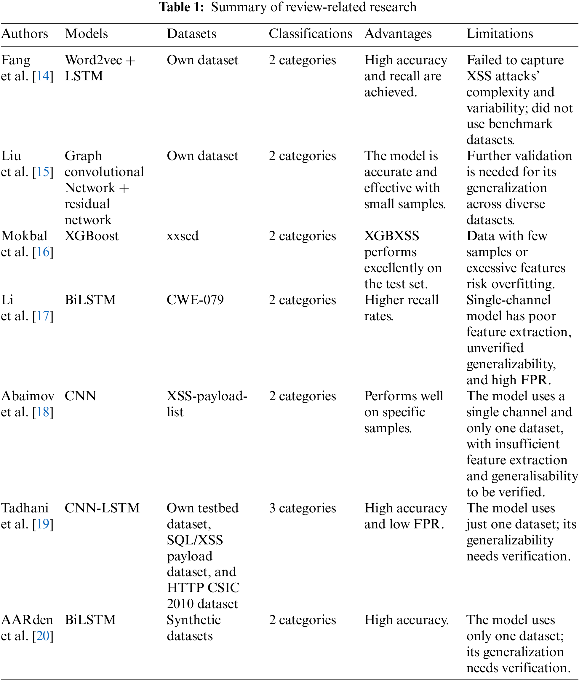
Fang et al. [14] introduced a deep learning-based XSS attack detection method, utilizing Word2vec to extract features from XSS payloads and conduct model training and testing with a long short-term memory Recurrent Neural Network (RNN). Although this method demonstrates high accuracy and recall on real datasets, Word2vec may not adequately capture specific script structures or the complex patterns of XSS attacks during feature extraction.

Liu et al. [15] developed a novel XSS load detection model utilizing graph convolutional networks and residual networks for feature analysis and identification. The model enhances detection accuracy by preprocessing the data and constructing graph structures. Although the model exhibits strong performance in small sample tests, its ability to generalize across a broad and diverse dataset requires further validation.

Mokbal et al. [16] developed an XSS attack detection framework named XGBXSS, which utilizes an Extreme Gradient Boosting (XGBoost) algorithm and advanced parameter optimization techniques. The framework enhances computational efficiency and significantly boosts detection performance through an advanced feature extraction method and a feature selection strategy that integrates information gain with sequential backward selection. Although XGBXSS demonstrates strong performance on the test set, it faces the risk of overfitting when dealing with limited samples or an excessive number of features.

Li et al. [17] developed an XSS vulnerability auditing method that combines a PHP code parsing tool and a Bi-LSTM model, which utilizes Word2vec to tag sequences and analyze the relationships between these sequences via a Bi-LSTM network. Their experiments demonstrated a recall of 0.98, significantly higher than the precision of 0.92, indicating that the method could possess a high FPR.

Abaimov et al. [18] developed a Convolutional Neural Network (CNN) model on the GitHub dataset that achieved accuracies of 95.7% and 90.2% in detecting SQL injection and XSS attacks, respectively. However, their model exhibits limited generalization capabilities when encountering new or unknown attack samples.

Tadhani et al. [19] introduced a hybrid deep learning network that combines CNN and LSTM, targeted at enhancing the protection of web applications against XSS and SQL injection attacks. However, this model may forfeit critical information during the concurrent feature extraction process involving CNN and LSTM.

The AARden team [20] proposed a deep learning approach incorporating BiLSTM, which successfully achieves accurate classification of XSS attacks, SQL injections, and normal requests by integrating manually labeled datasets for SQL injection and XSS attacks and employing multiple preprocessing strategies such as Porter stemming extraction and word embedding. However, the model only utilizes one dataset, thus its generalization performance needs to be verified.

In summary, the current research on XSS attack detection has made significant progress, with numerous scholars developing a variety of models based on advanced machine learning techniques. These models, spanning from combinations of Word2vec and LSTM using deep learning techniques to complex structures employing graph convolutional networks and residual networks, have demonstrated high accuracy and recall on specific datasets. However, these methods typically suffer from limitations such as insufficient generalization and inadequate capturing of complex attack patterns.

3  Methods

In this paper, we introduce a multi-stage XSS detection method that integrates Random Forest algorithm and CNN-POOL-BiLSTM to address several challenges. These challenges comprise complex feature processing, the limited adaptability of traditional methods, the susceptibility to overfitting in single-model neural networks, and inadequate annotations of the original XSS data.

In the primary stage of the model, the Random Forest algorithm is utilized to analyze the data deeply, identify its underlying structure and significant patterns, and generate a new feature set by extracting the leaf node indices of the Decision Tree (DT). These features are subsequently fused with the original data, forming an information-rich feature set. To further refine feature processing, the model incorporates three parallel channels operating independently. The first channel extracts multi-level local features in a 1D convolutional layer using three convolutional kernels of different sizes, enhancing the representational ability of these features through fusion techniques. The second channel focuses on identifying key features in the data through varying sizes of max 1D pooling layers. The third channel integrates a BiLSTM and a multi-head attention mechanism to effectively capture global information and improve understanding of long-term dependencies in the data. This multi-channel feature processing strategy not only enhances the accuracy and efficiency of the XSS attack detection model but also improves its adaptability and generalization in dealing with complex network environments. Its implementation is realized through four stages, as depicted in Fig. 1.

Figure 1: General framework of the model

(1) Step 1

The first step entails data pre-processing, which aims to ensure the quality and consistency of the data. This process comprises the removal of missing values, unique coding of the data, and normalization of the data.

(2) Step 2

In the second step, the Random Forest algorithm is used to dig deeper into the intrinsic structure and hidden patterns of the data. It is then used to generate leaf node indices as features of new dimensions. These newly generated features are incorporated into the original feature set, overcoming the problem of inadequate labelling of the original data, increasing the information content of the feature set and improving the expressiveness of the features.

(3) Step 3

The third step employs three parallel channels for additional feature extraction. Channel I utilizes parallel 1D convolutional layers, each with convolutional kernel sizes of 3, 5, and 7, for extracting local features across various scales and conducting multi-scale feature fusion. Channel II employs a max 1D pooling layer with kernel sizes of 3, 5, and 7 to extract pivotal features from the data, aiming to capture the most salient information. Channel III employs a Bi-LSTM to capture global information bidirectionally, which is combined with the multi-attention mechanism to further enrich the global information.

(4) Step 4

The fourth step is to overlay and fuse the features of the three channels, which not only combines the unique perspectives and information of each channel, but also enhances the diversity and richness of the features. This process allows the model to understand and represent the data in a more comprehensive way, improving the accuracy of the prediction and the model’s ability to generalise. Finally, a dense connectivity layer combined with an activation function is used to convert the integrated features of the network into probability distributions for each category to which the data belongs, leading to classification predictions.

4  Key Technologies for the Implementation of the Methodology

4.1 Data Pre-Processing

To ensure data quality, we employ data cleaning, one-hot encoding, and normalization techniques to uphold the validity and consistency of the data for subsequent analysis and modeling.

(1) Data Cleaning

When working with datasets, the initial step involves addressing extreme values representing positive and negative infinity, which may arise due to errors in data collection or computation. Given the mathematical instability and potential discrepancy with reality associated with these extreme values, their proper handling is essential to ensure the quality of the data. Therefore, we have adopted the strategy of replacing all such extreme values with NaN (not a numeric value) to identify anomalous data points. Lastly, to handle these missing values without eliminating any data rows, we opted to replace these NaNs with the average value of the corresponding data columns. This method yields a reasonable numerical estimate while preserving the overall statistical characteristics of the data.

(2) One-Hot Encoding

Given that certain datasets contain symbolic features, such as User Datagram Protocol (UDP), Transmission Control Protocol (TCP), Terminal Network (TELNET), File Transfer Protocol (FTP), we employ one-hot encoding to convert these symbolic features into numerical representations for subsequent analysis.

(3) Normalization

The primary objective of normalisation is to adjust the data to a consistent scale or range, thus improving model training efficiency and algorithm performance. This process entails reducing scale differences among different features, facilitating faster model convergence, bolstering model stability and robustness, and mitigating numerical instability issues. Normalisation boosts the resilience and efficiency of the model by ensuring a uniform scale among different features. The normalisation formula is given in Eq. (1).

xnew=xcurrent−xminxmax−xmin(1)

The variable xcurrent represents the original value to be normalized, denoted as the current value; xmin denotes the minimum value in the dataset; and xmax denotes the maximum value in the dataset.

4.2 Feature Expansion

To mitigate the negative impact of insufficient raw data annotation on the model’s learning effectiveness and generalization ability, we utilize the Random Forest algorithm for feature set expansion. The core of this approach lies in enhancing the data features through the multi-tree structure of Random Forest and the strategy of randomly selecting features. Specifically, we initially analyze the original dataset using the Random Forest algorithm to identify crucial features and underlying patterns. Based on this information, we generate new feature sets to enrich the original dataset. These new features not only improve the model’s ability to understand the data but also enhance its adaptability and generalization to new scenarios. This approach effectively enhances the model’s performance when confronted with inadequately annotated raw data. The specific implementation process is as follows:

(1) Bootstrap sampling: Initially, the original dataset D is partitioned into a training set and a test set based on a specific ratio. Subsequently, bootstrap sampling is employed to extract N subsets DN from the training dataset, each utilized for training individual trees within the Random Forest.

(2) Compute the gini inequality: For each subset DN, calculate its Gini impurity G(DN). The Gini impurity G(DN) serves as a metric for the level of classification ambiguity within the dataset and the calculation formula is shown in Eq. (2).

G(DN)=1−∑j=1Jpj2(2)

where pj represents the proportion of samples belonging to the j-th category in the dataset DN, and J denotes the total number of categories.

(3) Splitting trees: During the DT construction process, the algorithm selects features that most effectively reduce the Gini impurity to serve as split nodes. At each node, the algorithm traverses through all features and their potential split points, computes the weighted Gini impurity following the split, and identifies the features and split points that minimize the weighted Gini impurity. The weighted Gini deprivation is calculated according to Eq. (3).

ΔG(DN,A)=G(DN)−∑i=1k|DNi||DN|G(DNi)(3)

Here, A represents the feature under consideration, while DNi denotes the subset obtained after segmentation based on a specific segmentation point of feature A, with k representing the number of subsets.

(4) Recursive splitting: The above process is repeated, recursively applying the Gini impurity calculation and optimal feature selection to each split child node until a certain stopping condition is satisfied, e.g., the maximum depth of the tree is reached.

(5) Construction of the Random Forest: By iterating through the aforementioned steps on various subsets of DN, multiple DTs are constructed to constitute a Random Forest.

(6) Leaf node path retrieval: Within each DT of a Random Forest, every sample is allocated to a leaf node. We record the entire path taken by each sample to reach the leaf node. This path reflects the sample’s splitting history within the DT, encompassing the testing conditions of every traversed node.

(7) Extended feature set: The leaf node paths of every sample are converted into a novel feature set. More precisely, the path information of each sample within the DT, comprising the node indices traversed, the splitting features employed at each node, and the splitting threshold, is utilized for generating a novel feature set. Consequently, the original feature set is enriched into a more comprehensive feature set that incorporates information about DT paths.

4.3 Channel I

To extract local information from XSS data, a 1D convolutional neural network is employed. This network utilizes a 1D convolutional operation to learn and extract local features from the input data. The formula is given by Eq. (4).

xjl=f(∑i=1Mxil−1∗kijl+bjl)(4)

Here, xjl represents the output of neuron j in the lth 1D convolutional layer. The activation function f, in this paper, is the softmax function used to introduce nonlinearity. The convolution operation is denoted by ∑i=1Mxil−1∗kijl, where xil−1 represents the output of neuron i in the (l-1)th layer and kijl is the weight connecting neuron i in the (l-1)th layer to neuron j in the lth layer. Additionally, bjl represents the bias term of neuron j in the lth layer of the 1D convolutional layers.

For comprehensive coverage of the region of interest by the CNN output, precise control of the receptive field becomes imperative. Therefore, we employ convolutional kernels of varying sizes, processed concurrently, to extract features across different scales. This strategy enables the network to focus on both the intricacies of local structures and the nuances of details. In the initial channel, a parallel 1D convolutional layer is introduced with convolutional kernels of sizes 3, 5, and 7, each with depths of 32, 64, and 128, respectively. This configuration facilitates the simultaneous extraction of diverse local attack features. Smaller convolutional kernels excel at capturing local structures and finer details, while larger ones are adept at grasping long-range dependency information. Such a design comprehensively enhances the network’s understanding of the input data, thereby refining feature perception across various scales.

4.4 Channel II

To prioritize the extraction of crucial features from the XSS data, we incorporate a max 1D pooling layer into the model. This layer enables the model to concentrate on the most significant and informative features by selecting the maximum value from each pooled region. This systematic approach effectively emphasizes the pivotal aspects of the data, ensuring that the model captures features essential for the final task. Consequently, the model’s capability to identify and utilize key information across diverse datasets is enhanced.

yj=max(x(j−1)⋅s+1,…,x(j−1)⋅s+k)(5)

where yj is the jth element in the pooled output sequence, k is the size of the pooling window, and s is the step size.

In this study, three different sizes of max 1D pooling layers are employed, specifically sizes 3, 5, and 7. There are several advantages to incorporating pooling layers of varying sizes. Firstly, they facilitate the capture of features across multiple scales: smaller pooling layers excel at capturing finer-grained features, while larger ones encompass a broader range, ensuring comprehensive coverage of important information across all levels. Secondly, this multi-scale feature extraction enhances the model’s generalizability by enabling the capture of diverse features across different pooling layers, thereby augmenting the model’s ability to generalize to new data.

4.5 Channel III

To comprehensively extract global information from XSS data, we employ a cutting-edge approach that integrates BiLSTM networks with multi-head attention mechanisms. This fusion significantly enhances the model’s performance in handling complex data structures, particularly excelling in tasks requiring the understanding of long-range dependencies and multi-dimensional information.

4.5.1 BiLSTM

For the extraction of global features from XSS data, we employ the BiLSTM network, which enhances data comprehension by integrating two LSTM networks. LSTM, a specialized form of RNN, is adept at capturing long-term dependencies within sequences through feedback connections. It operates by storing pertinent information in memory cells while discarding redundant data, thereby outperforming conventional RNNs. The architecture of an LSTM’s memory cells, as depicted in Fig. 2, comprises a single memory cell alongside three gates: the forgetting gate, the input gate, and the output gate, each delineated as follows.

Figure 2: LSTM model

Oblivion Gate: The Oblivion Gate determines which information should be discarded from the cell state. As depicted in the following equation, ft represents the information to be retained (close to 1) and the information to be forgotten (close to 0).

ft=σ(Wf⋅[ht−1,xt]+bf)(6)

Input Gate: The old cell information Ct−1 is updated to the new cell information Ct. The update process involves selecting a portion of the old cell information to be discarded by the Forget Gate, and choosing a segment of the candidate cell information Ct~ to be included by the Input Gate to obtain the new cell information Ct.

it=σ(Wi⋅[ht−1,xt]+bi)(7)

Ct~=tanh(WC⋅[ht−1,xt]+bC)(8)

Ct=ft∗Ct−1+it∗Ct~(9)

Output gate: To determine the states characterizing the output cell based on the inputs ht−1 and xt, it is necessary to pass the inputs through the sigmoid layer of the output gate to obtain the attenuation coefficient ot and then multiply them by the scaled memory state Ct to derive the output information at time t (that is, the hidden state ht).

ot=σ(Wo⋅[ht−1,xt]+bo)(10)

ht=ot∗tanh⁡(Ct)(11)

Here, bf, bi, bc, and bo represent the bias vectors, while Wf, Wi, Wc and Wo denote the weight matrices. The activation function for the gate is σ(.), which is a logistic sigmoid function, while tanh(.) serves as the activation function for the input and output modules.

BiLSTM, an extended version of LSTM, analyzes data by integrating two LSTM layers: a forward layer and a backward layer. The forward layer processes the original data sequence, capturing temporal dependencies from the beginning to the end, while the backward layer processes the sequence in reverse order, capturing temporal dependencies from the end to the beginning. The simultaneous application of LSTM layers enhances the model’s ability to learn long-term dependencies, thereby improving detection accuracy. Therefore, in this paper, we utilize BiLSTM to extract global features from XSS data.

4.5.2 Multiple Attentional Mechanisms

To augment the global features, we employ the multi-head attention mechanism. The multi-head attention mechanism, a variant of the attention mechanism, constitutes a crucial component of the neural network architecture, offering a method to allocate distinct weights to the input data for feature extraction. Self-attention is computed as follows: initially, a linear mapping is executed for each token in the input token sequence to derive a collection of query vectors (Q), key vectors (K), and value vectors (V). For each token, the Q is utilized to interrogate (multiply) the K of other tokens, obtaining the correlation value of that token with other tokens in the sequence. The formula is shown in Eq. (12).

Attention(Q,K,V)=softmax(QKTdk)V(12)

dk represents the embedding dimension K. For a large dimension, the dot product’s result magnifies, leading to saturation in the region of the softmax activation function, thereby causing a diminishing gradient. Thus, following the dot product, the outcomes Q and K are divided by dk to prevent gradient vanishing.

As shown in Fig. 3, multi-head self-attention is an extension of the attention mechanism that utilizes multiple parallel attention heads to simultaneously capture information from multiple subspaces. Initially, it conducts h distinct linear projections of queries, keys, and values, executing attention in parallel to generate outputs in the dimension (dV/h). Subsequently, these outputs are concatenated to yield the final values. The expression for multi-head self-attention is as follows:

MultiHead(Q,K,V)=Concat(head1,⋯,headh)WO(13)

headi=Attention(QWiQ,KWiK,VWiV)(14)

Figure 3: Results of the multi-attention mechanism

Here, headi represents the computation result of the ith attention head. WiQ, WiK, WiVdenote the transformation matrices of Q, K, and V of the ith head, respectively. Additionally, WO is utilized to transform the output of the multi-head self-attention back to the original dimension of the token.

Utilizing BiLSTM to capture long-term dependencies from both positive and negative directions, while simultaneously incorporating the multi-headed attention mechanism, enhances the model’s capability to attend to various parts of the data. This enables the model to comprehend and extract key features comprehensively from multiple perspectives, facilitating a more thorough understanding of the data. This multifaceted and in-depth information processing not only enhances the model’s comprehension of complex data structures but also significantly heightens its sensitivity to subtle information and efficiency in extracting global information, thereby rendering the model more effective and accurate in processing data with intricate dependencies.

5  Experimental Validation and Result Analysis

To validate the effectiveness of our proposed model, we conducted extensive experiments on six datasets. In these experiments, we not only compared our CNN-POOL-BiLSTM network model with four classical algorithms—K-Nearest Neighbors (KNN), Naive Bayes (NB), Logistic Regression (LR), and DT, but also executed a series of ablation experiments to demonstrate the validity of the innovations in our model. Additionally, we compared our model with the latest models proposed in the last two years to further demonstrate its performance and advantages. Through these comprehensive experiments and comparative analyses, we validated the effectiveness and advancement of our model in all aspects.

5.1 Datasets

Extensive experiments were conducted on four public datasets. The first dataset, published by Mokbal et al. [21] and updated in 2021 [16], is considered to be the first comprehensive digital signature dataset based on XSS extracted from real-world XSS attacks. The benign samples in this dataset were generated by crawling the top 50,000 Alexa-ranked websites, while the malicious samples were collected by crawling raw XSS repositories such as XSSed and Open Bug Bounty. Additionally, the dataset contains 66 numerical features.

The second dataset represents an updated version of the initial dataset. In comparison to the initial dataset, the second dataset encompasses a greater number of numerical features, totaling 167, rendering it more informative for conducting in-depth analysis of XSS attacks. While both datasets are constructed similarly, with benign samples extracted from high-traffic websites and malicious samples sourced from publicly available XSS vulnerability repositories, the second dataset offers a more comprehensive perspective for investigating XSS attacks through the expansion of its feature set.

The third dataset, known as the CICIDS2017 dataset, stands as one of the most renowned intrusion detection datasets compiled by the Canadian Institute for Cybersecurity Research [22]. This dataset is meticulously crafted to address the limitations of existing datasets and furnish a realistic and dependable resource for intrusion detection [23]. The CICIDS2017 dataset encompasses attacks captured from Monday, 3rd July, 2017, to Friday, 7th July, spanning a total of 5 days and including benign as well as recent common attacks. The CICIDS2017 dataset comprises 8 distinct files, totaling 2,830,743 records, with each record containing 80 features. The entire dataset comprises 14 diverse types of attacks, including Denial of Service attacks (DoS), Web Attacks, Brute Force Breach, Heartbleed, Penetration, Botnets, PortScan, and Distributed Denial of Service attacks (DDoS). Due to the substantial volume of data and classes, there is increased overhead for loading and processing. Hence, we opted to process four of these files.

The fourth dataset, known as the UNSW-NB15 dataset, was generated by the IXIA PerfectStorm tool at the Australian Centre for Cyber Security (ACCS) CyberScope Lab [24] and stands as one of the most popular datasets currently utilized. This dataset comprises 257,673 records, wherein 63.9% correspond to network flows representing nine types of attacks (Generic, Exploit, Fuzzer, DoS, Reconnaissance, Analytics, Backdoor, ShellCode, Worms), with the remaining 37.1% representing normal network connections. Each record in this dataset is composed of 49 features, among which two are designated for multi-class and binary labelling purposes. Among the remaining 47 features, 45 are numeric, while the remaining 2 are class features.

We created the fifth dataset. To assess the applicability of our model in real network environments, we adopted a method involving the simulation of actual network attacks. In this experimental setup, two virtual machines were configured, one designated as the attacker and the other as the victim. On the victim virtual machine, we established an xss-lab platform for XSS testing, whereas on the attacker virtual machine, we performed various operations, including XSS attacks and normal access. Throughout the test, the tcpdump tool was run on the victim VM to capture all network traffic. Following this, the CICFLOWMETER tool was utilized to extract features from this traffic data, resulting in a dataset comprising 2033 entries, of which 1006 were classified as normal traffic and 1027 as XSS attack traffic. By constructing this simulation environment and dataset, we were able to precisely evaluate our model’s capability to detect XSS attacks and its efficacy in discerning between normal and malicious traffic, without perturbing the actual network environment.

The sixth dataset, NSL-KDD [25], is an enhanced version of the renowned KDD Cup. It serves as a crucial benchmark dataset for evaluating Network Intrusion Detection System (NIDS) algorithms. NSL-KDD comprises two parts: KDDTrain+ and KDDTest+. The training set comprises 125,973 samples, of which 67,343 are labeled as “normal” and 58,630 as “abnormal”, encompassing 22 attack types categorized into 4 attack categories. The test set comprises 22,544 samples, with 9711 labeled as “normal” and 12,833 as “abnormal”, covering 37 attack types, likewise categorized into 4 attack categories. The four categories include: DoS, Root-to-local attacks (R2L), User-to-root attacks (U2R), and Probe attacks (Probe).

5.2 Evaluation Indicators

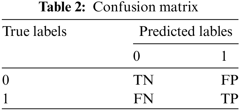
Following the analyses, we assessed the performance of our method using various evaluation metrics, including model Accuracy, Precision, Recall, F1 score, FPR, and False Negative Rate (FNR). We computed the confusion matrix, which includes True Positive (TP), True Negative (TN), False Positive (FP), and False Negative (FN), as demonstrated in Table 2:

Accuracy represents the ratio of all correctly labeled classes to the total number of classifications and is calculated using Eq. (15).

Accuracy=TP+TNTP+TN+FP+FN(15)

Precision is a measure of how many of the predicted positive instances are actually positive. Precision is calculated using Eq. (16).

Precision=TPTP+FP(16)

Recall represents the ratio of correctly predicted positive instances to all instances that are actually positive. It is calculated as shown in Eq. (17).

Recall=TPTP+FN(17)

The F1 score is a measure of accuracy used to evaluate precision and recall. It is the harmonic mean of precision and recall, and the F1 score is calculated according to Eq. (18).

F1=2×Precision×RecallPrecision+Recall=2×TP2×TP+FP+FN(18)

FPR is the proportion of samples that are actually negative instances in the classification model that are incorrectly predicted to be positive instances. FPR is calculated as shown in Eq. (19).

FPR=FPFP+TN(19)

FNR represents the ratio of positive samples incorrectly classified as negative to all samples that are actually positive. FNR is calculated as shown in Eq. (20).

FNR=FNFN+TP(20)

5.3 Experimental Setup

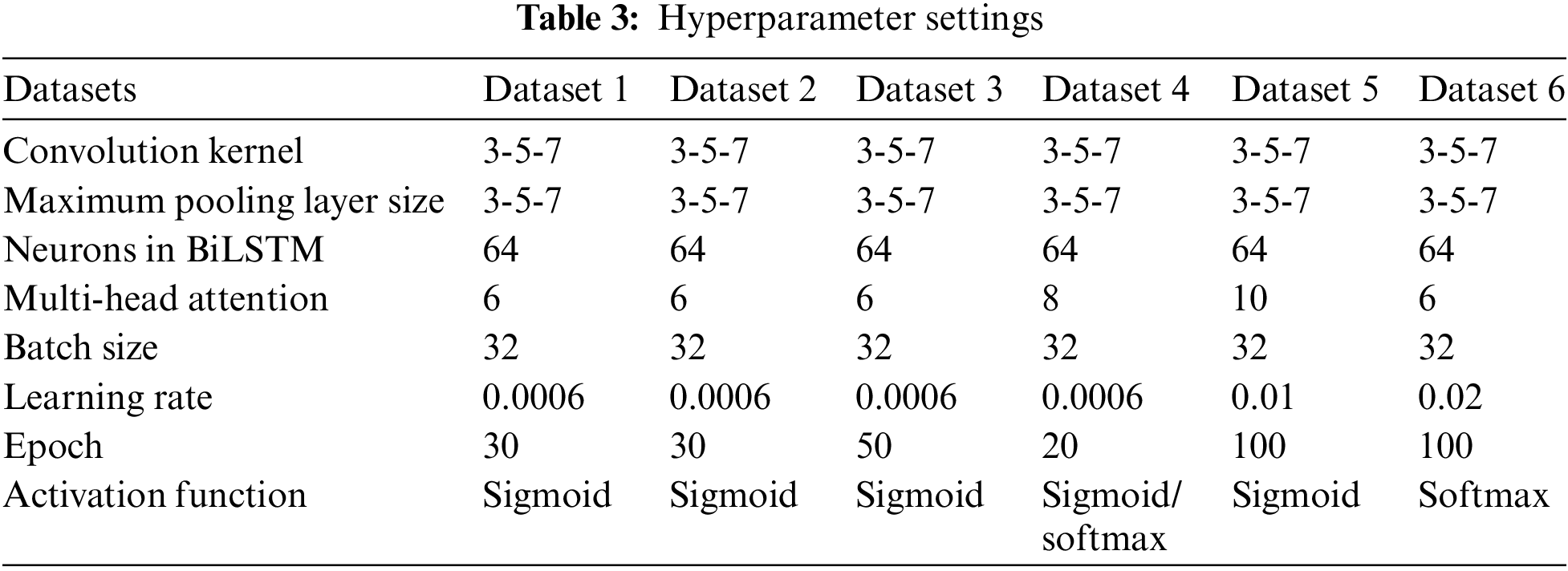
In this study, all six datasets were systematically partitioned into training, validation, and test sets, where the training set comprised 80% of the total data, the validation set comprised 10%, and the testing set comprised 20%. This approach facilitates a comprehensive evaluation of the model’s performance. Moreover, the Adam optimizer is employed during model training to ensure both the efficiency and stability of the optimization process. Table 3 presents the detailed hyperparameter configuration adopted for each dataset. In addition, we use the cross-entropy loss function to improve the prediction accuracy of the model.

5.4 Comparison of Experimental Results and Analysis with Four Classical Algorithms

To verify the performance and adaptability of our CNN-POOL-BIATTEN model, exhaustive experiments were conducted on six selected datasets. First, Dataset 1 and Dataset 2 were utilized to evaluate the model’s binary classification accuracy in XSS detection when processing both basic and extended features. Subsequently, the model’s binary classification detection effect was tested across datasets by using Dataset 3 (CICIDS2017) and Dataset 4 (UNSW-NB15) to evaluate its generalization ability. It is worth noting that Dataset 5 was specifically created to assess the model’s performance in distinguishing XSS attacks from normal traffic by simulating a real network environment, thus ensuring its effectiveness in practical application scenarios. Additionally, multi-classification tests were conducted on Dataset 4 and Dataset 6 (NSL-KDD) to further investigate the model’s capability in handling diverse types of complex network attacks. For comprehensive evaluation, the model’s performance was compared with four classic algorithms—KNN, NB, LR, and DT. The results are summarized as follows.

5.4.1 Two categories

(1) Dataset 1

The results of the calculations on dataset 1 are shown in Table 4.

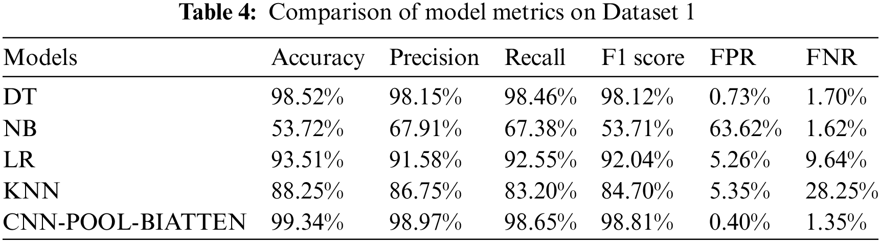
The CNN-POOL-BIATTEN model demonstrates superior performance over other conventional models in almost all metrics, particularly in accuracy (99.34%) and F1 score (98.81%). Additionally, the model significantly reduces the FPR (0.40%) and FNR (1.35%). However, despite DT’s good accuracy performance, its performance in other metrics does not match that of CNN-POOL-BIATTEN. NB exhibits the worst overall performance among all models, particularly in terms of the FPR, which is significantly higher than that of the other models. These results suggest that the CNN-POOL-BIATTEN model offers significant advantages in handling complex datasets and performing high-precision classification tasks.

(2) Dataset 2

The results of the calculations on Dataset 2 are shown in Table 5.

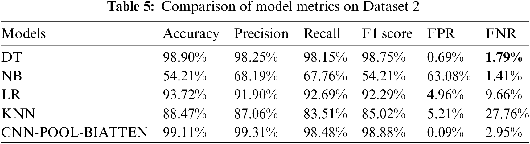
The CNN-POOL-BIATTEN model demonstrates significant superiority in all core performance metrics, with an accuracy of 99.11%, a precision of 99.31%, a recall of 98.48%, and an F1 score of 98.88%. These metrics collectively demonstrate its excellent capability to accurately identify positive categories and mitigate misclassifications. Additionally, its FPR of only 0.09% and FNR of 2.95% further highlight its efficiency in error control. In comparison to CNN-POOL-BIATTEN, DT exhibits a lower FNR but slightly inferior performance in other metrics. The performance of the NB model significantly lags behind, suggesting that it does not handle complex data feature dependencies well enough. The LR and KNN models exhibit relatively high FNR, suggesting significant challenges in distinguishing positive class samples and indicating limitations in handling this dataset. Therefore, the CNN-POOL-BIATTEN model performed best.

(3) Dataset 3

The results of the calculations on Dataset 3 are shown in Table 6.

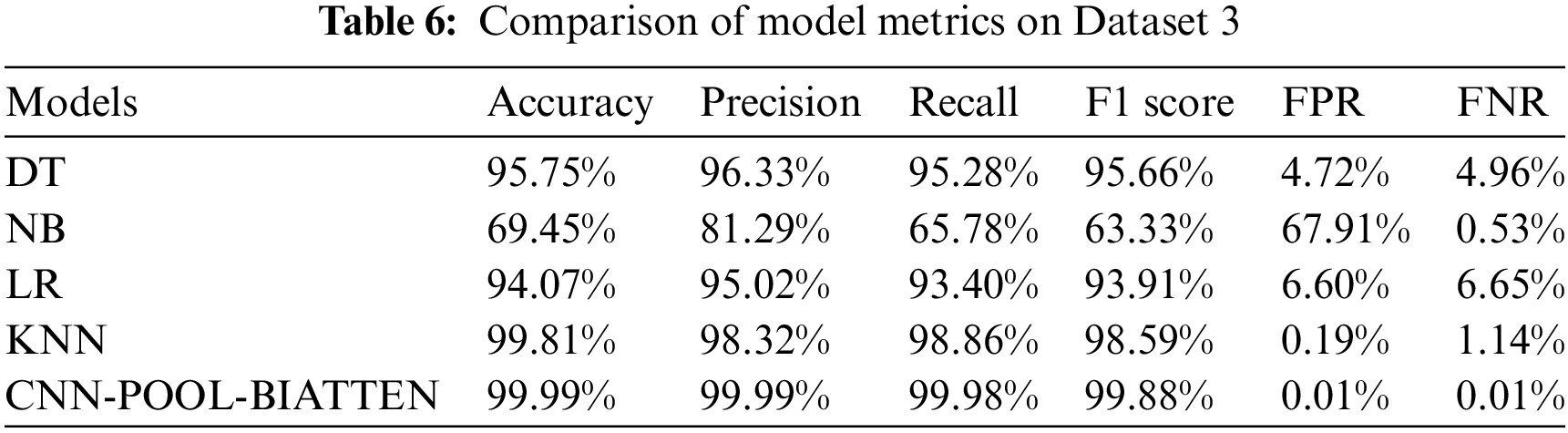
The results indicate that the CNN-POOL-BIATTEN model demonstrates a clear advantage in handling complex data, especially when compared to other models. The performance of the model approaches perfection in almost all key metrics, including an accuracy of 99.99%, precision of 99.99%, recall of 99.98%, and an F1 score of 99.88%, as well as an exceptionally low FPR and FNR of 0.01%, which further underscores its superior performance in terms of accuracy and reliability. In contrast, the DT, NB, and LR models exhibit relatively high FPR, which accentuate their shortcomings in capturing key features. The KNN model, on the other hand, demonstrates its pattern recognition power with an accuracy of 99.81% and an F1 score of 98.59%, yet it is slightly inferior to the CNN-POOL-BIATTEN model in terms of overall performance. Overall, our CNN-POOL-BIATTEN model significantly surpasses the other models in several key performance metrics, especially in terms of efficiency and reliability in reducing FPR and omissions, thus underscoring its strong potential in dealing with complex datasets.

(4) Dataset 4

The results of the calculations on Dataset 4 are shown in Table 7.

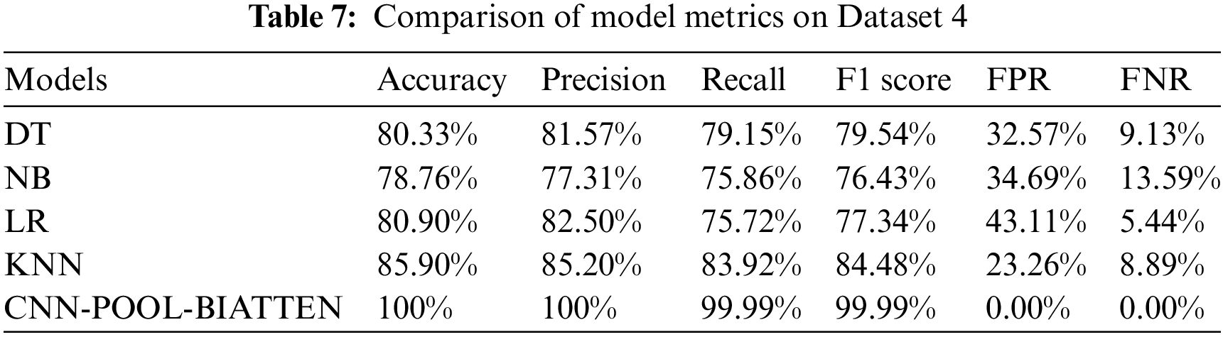
The CNN-POOL-BIATTEN model excels in nearly all metrics, boasting a precision of 100% and achieving zero FPR and FNR. This underscores its flawless recognition capability in classification tasks. In contrast, the KNN model performs well among traditional models, with an accuracy of 85.90%, an F1 score of 84.48%, a lower FPR of 23.26%, and a higher recall of 83.92%, demonstrating its effectiveness in positive category recognition. The LR model performs moderately well in terms of both accuracy and precision. However, its high FPR of 43.11% highlights potential shortcomings in distinguishing negative categories. The DT model performs in the middle range, with an accuracy of 80.33% and an F1 score of 79.54%, indicating a certain degree of reliability. However, its relatively high FPR suggests that there is still room for optimization in handling this dataset. In contrast, the NB model is the poorest performer among all traditional models, with lower accuracy and F1 scores of 78.76% and 76.43%, respectively. Additionally, it exhibits a FPR of 34.69% and a FNR of 13.59%, clearly indicating its shortcomings in predictive accuracy. These comparative results underscore the significant advantages of CNN-POOL-BIATTEN in dealing with complex classification problems.

(5) Dataset 5

The results of the calculations on Dataset 5 are shown in Table 8.

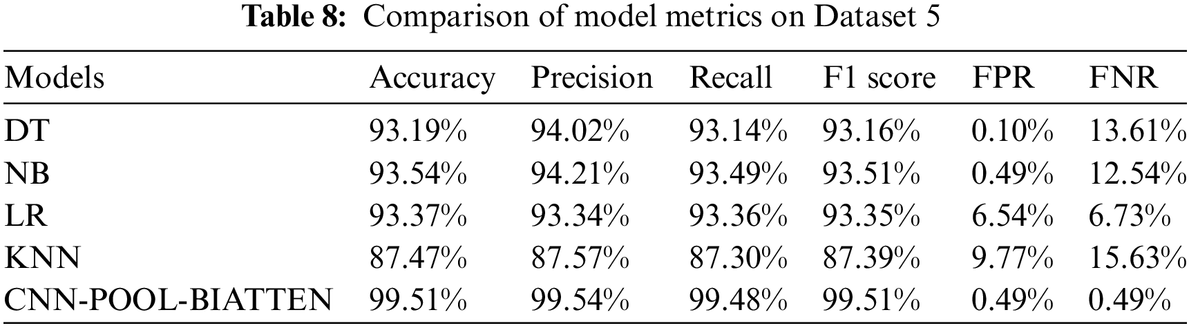
The CNN-POOL-BIATTEN model demonstrates significant improvement in all performance metrics compared to traditional machine learning models such as DT, NB, LR, and KNN. Specifically, the model attains or surpasses 99.4% in accuracy, precision, recall, and F1 score, significantly outperforming other models and highlighting its superior efficacy in complex pattern recognition and data feature extraction. Additionally, its FPR and FNR are maintained at 0.49%, demonstrating that CNN-POOL-BIATTEN offers enhanced stability and reliability in minimizing FPR and omissions.

5.4.2 Multi-Category

(1) Dataset 4

Highly unbalanced datasets may adversely affect model performance. Given that unbalanced datasets are not central to this study, we excluded four minority categories: ‘Analytics’, ‘Backdoor’, ‘Shellcode’, and ‘Worms’, which comprise only 1.141%, 0.996%, 0.646%, and 0.074% of the training set, respectively. The results of the multi-category experiments for Dataset 4 are presented in Table 9.

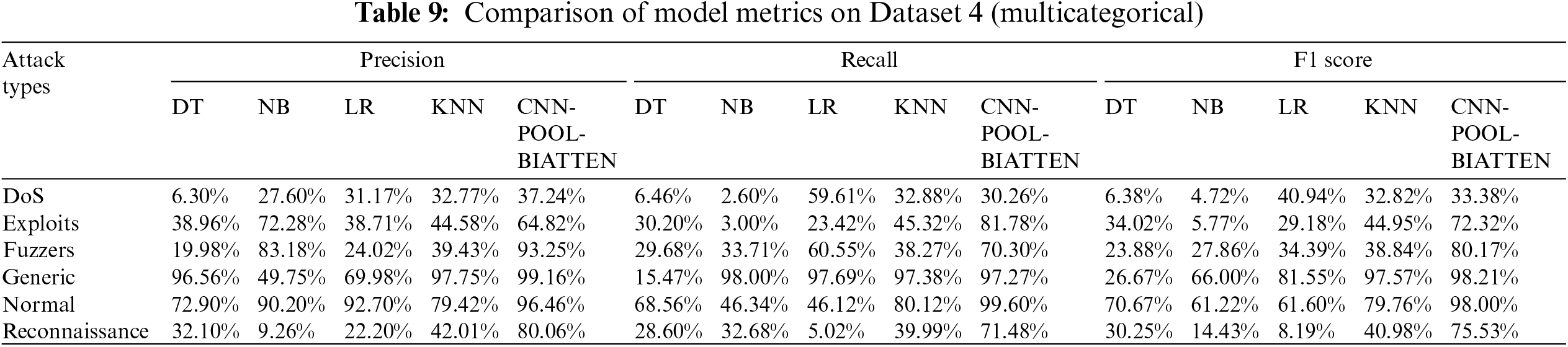
It is evident that the CNN-POOL-BIATTEN model exhibits strong performance in terms of precision, recall, and F1 score across various attack types, particularly with complex attacks such as Generic and Fuzzers. For instance, for the Generic attack type, CNN-POOL-BIATTEN achieves a precision of 99.16%, a recall of 97.27%, and an F1 score of 98.21%, positioning it as the top performer among all models. Additionally, in the challenging Exploits and Reconnaissance attack types, CNN-POOL-BIATTEN demonstrates high recall and F1 scores, evidencing its robustness and adaptability against diverse attack patterns.

(2) Dataset 6

The results of the calculations on Dataset 6 are shown in Table 10.

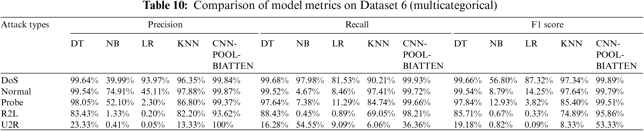
It is evident that the CNN-POOL-BIATTEN model exhibits outstanding performance compared to other models, particularly in addressing DoS and Probe attacks, where its precision, recall, and F1 scores exceed 99%, demonstrating an exceptionally high recognition capability. The model further demonstrates superior performance in the detection of normal traffic and R2L attacks, particularly in the nearly flawless identification of normal traffic. Additionally, even in the U2R attack category, which has fewer samples, the model achieves 100% precision, although the recall is low. Overall, the CNN-POOL-BIATTEN model demonstrates significant advantages in the identification and classification of network attacks.

5.5 Loss Functions and Accuracy Curves

To further demonstrate the model’s adaptability and generalization ability in handling data of various types and complexities, we recorded the training and validation loss values and accuracy for each epoch of the first four datasets. Subsequently, we plotted them as curves, represented in Figs. 4–7.

Figure 4: Loss curves and accuracy curves for the training and test data for Dataset 1

Figure 5: Loss curves and accuracy curves for the training and test data for Dataset 2

Figure 6: Loss curves and accuracy curves for the training and test data for Dataset 3

Figure 7: Loss curves and accuracy curves for the training and test data for Dataset 4

In Figs. 4 and 5, the model demonstrates excellent stability across Dataset 1 and Dataset 2. The rapid decrease in the loss function and the steady increase in accuracy indicate that the model exhibits remarkable adaptability to the training data. This robustness suggests that the model effectively avoids overfitting during training and maintains strong generalization ability. Fig. 6 illustrates some fluctuations in the model’s performance during training on Dataset 3, which also underscores its flexibility and adaptability. Despite these fluctuations, the model maintains relatively high accuracy even when dealing with potentially more complex or noisy data. Fig. 7 further demonstrates the model’s strong performance and generalization capability on Dataset 4. In the initial stages of training, there is a rapid decrease in loss accompanied by a sharp increase in accuracy, indicating the model’s ability to quickly learn and adapt to the data. As training progresses, both the loss and accuracy curves stabilize, and the model’s performance on the validation set remains consistent with that on the training set, indicating no signs of overfitting or underfitting. Ultimately, the model achieves near-perfect accuracy levels, underscoring its efficiency and reliability in classification tasks. Overall, the model exhibits robustness and efficiency across various datasets, demonstrating its strong learning ability and generalization potential.

5.6 Ablation Experiments

To validate our innovation, we performed a series of ablation experiments on the first four datasets. Initially, in the Random Forest feature enhancement ablation experiment, we intentionally omitted this aspect of the Random Forest feature enhancement to evaluate its specific impact on the overall model performance. This step is intended to elucidate the role and significance of Random Forest feature enhancement in the overall model architecture. By comparing the model’s performance before and after the removal, we can gain a clearer understanding of the practical utility of this innovation. Subsequently, a more detailed approach was taken in our three-channel ablation experiments. In this series of experiments, each channel was individually removed while keeping the other two intact, enabling the assessment of each channel’s contribution independently. The objective is to precisely quantify the impact of each channel on model performance. This methodology not only identifies the most critical channel but also uncovers potential synergies between them.

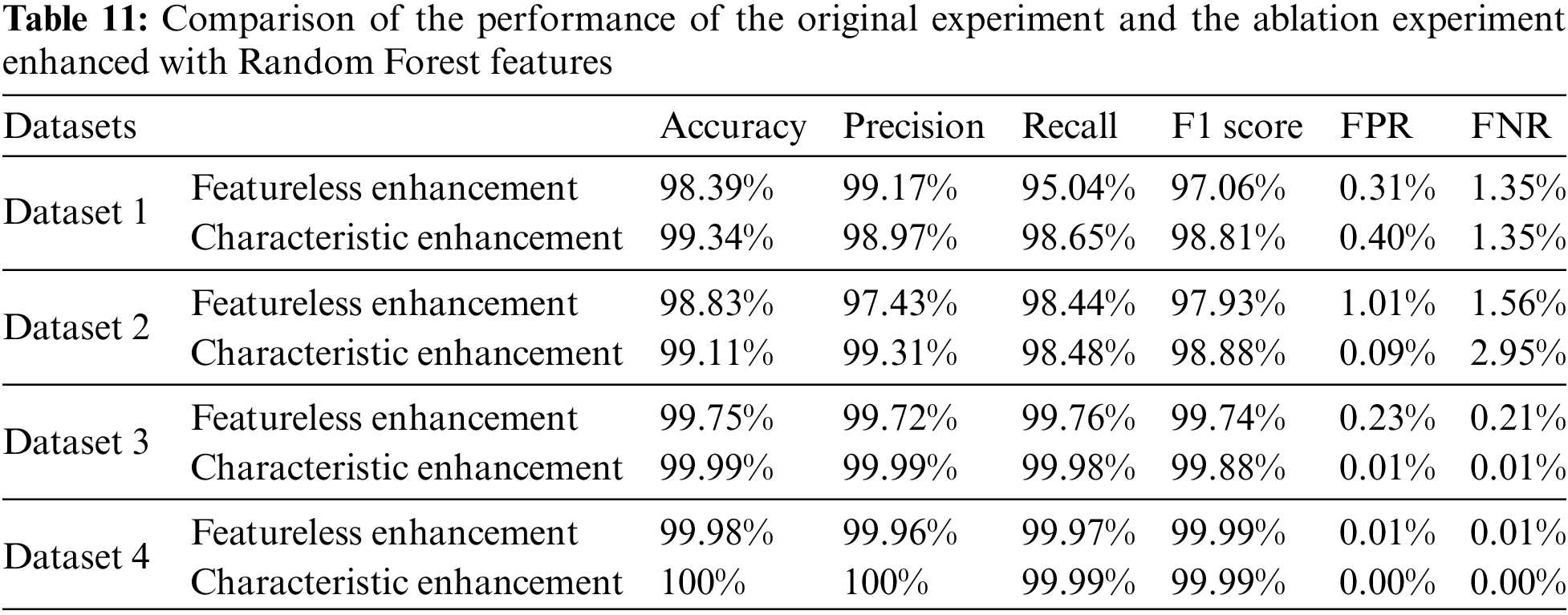
5.6.1 Ablation Experiments with Random Forest Feature Enhancement

As shown in Table 11, the results of the ablation experiments of the Random Forest feature enhancement technique on different datasets demonstrate its significant advantages in improving model performance. Specifically, the experiments on Dataset 1 show that feature enhancement increases the accuracy of the model from 98.39% to 99.34% and the F1 score from 97.06% to 98.81%, fully demonstrating the positive effect of feature enhancement in improving the overall performance of the model. Despite the decrease in the accuracy rate and the slight increase in the FPR, these changes are acceptable in the context of the overall performance improvement. Meanwhile, the increase in recall further illustrates the effectiveness of Random Forest in improving the model’s ability to identify positive classes. In Dataset 2, the improvements in accuracy and F1 score also highlight the important role of feature enhancement in fine-tuning model performance. The experimental results in Dataset 3 and Dataset 4 show that feature enhancement brings some improvement in almost all evaluation metrics. In conclusion, the Random forest feature enhancement technique improves model performance to varying degrees.

5.6.2 Ablation Experiments in Three Channels

Based on a comprehensive analysis of the provided data, clear distinctions in the performance of various channel combinations across the four datasets are evident, highlighting the considerable benefits derived from the integration of Channels 1, 2, and 3, as depicted in Table 12.

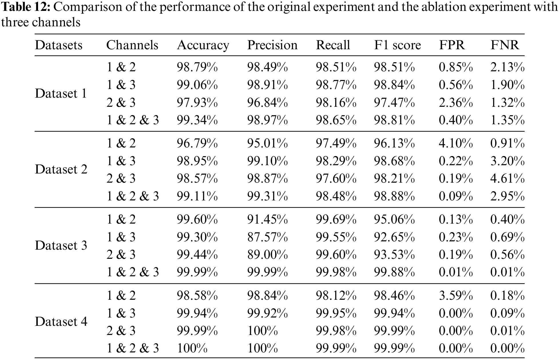
On Dataset 1, the combination of Channel 1 and Channel 2 exhibited high accuracy (98.79%) and F1 score (98.51%), albeit with slightly inferior overall performance compared to the three-channel combination (99.34% accuracy and 98.81% F1 score). Particularly notable were the lower FPR observed in the three-channel combination. Furthermore, the combination of Channel 1 and Channel 3 demonstrated higher accuracy and F1 score, leveraging the local feature extraction of Channel 1 and the global information processing of Channel 3 effectively, thereby demonstrating the complementary nature of features across different channels.

On Dataset 2, the combination of Channel 1 and Channel 2, while achieving higher accuracy (96.79%) and recall (97.49%), exhibits slightly lower precision (95.01%) and F1 score (96.13%), indicating limitations in detailed classification. The combination of Channel 1 and Channel 3, as well as the combination of Channel 2 and Channel 3, exhibit higher accuracy and precision rates, respectively. Particularly, the combination of Channel 2 and Channel 3 demonstrated almost error-free performance in distinguishing negative categories. The combination of all three channels results in a significant improvement in overall performance, with an accuracy of 99.11% and an F1 score of 98.88%, highlighting the advantages of integrating the characteristics of different channels.

The analysis of Dataset 3 shows that the combinations of Channel 1 and Channel 2 as well as Channel 1 and Channel 3, although excellent in terms of accuracy and recall, are slightly less accurate in terms of precision and have a high FPR. The combination of Channel 1 and Channel 2 had a high accuracy (99.60%) but a low precision (91.45%). On the contrary, the combination of all three channels achieves perfect performance (99.99%) on almost all metrics, which significantly reduces FPR and omissions, highlighting the importance of multi-channel feature extraction strategies.

The analysis in Dataset 4 shows that the combination of Channel 1 and Channel 2 performs well in terms of accuracy (98.58%) and F1 score (98.46%), but it performs poorly in terms of reducing FPR. On the contrary, the combination of Channel 1 and Channel 3 as well as Channel 2 and Channel 3 performs almost perfectly in terms of accuracy, precision, and recall. Meanwhile, the combination of all three channels achieves perfect performance on Dataset 4 with 100% accuracy and precision, demonstrating the effectiveness of the multi-channel strategy in improving model performance.

The results of these analyses highlight the importance of applying multi-channel feature extraction strategies when processing complex datasets. While single-channel or two-channel combinations perform well on specific metrics, they usually fail to achieve the overall performance of three-channel combinations. The three-channel combination enhances the performance of the model in all aspects and significantly enhances the generalisation ability of the model by combining the accurate capture of local details with the processing of global information. This strategy is crucial when dealing with complex datasets that require multiple feature types to be considered simultaneously, and it can effectively improve the accuracy, precision, and stability of the model.

5.7 Comparison Experiments with the Latest Model

We also compared our model with the latest models proposed in the last two years on the same dataset, to comprehensively evaluate the competitiveness and innovativeness of our model. The experimental results and analyses are presented below, with the literature results for comparison extracted from the original papers.

(1) Dataset 1

As shown in Table 13, the Deep Q-Network model of Thajeel et al. [2] integrates deep and reinforcement learning techniques with a multi-intelligent body feature selection algorithm, specifically designed for dynamically detecting and responding to XSS attacks. The model achieves a high accuracy of 99.59% on Dataset 1 by incorporating an innovative multi-intelligent body system for dynamic feature optimization. However, when compared with our CNN-POOL-BIATTEN model on the same dataset, the CNN-POOL-BIATTEN model demonstrates superior performance in key performance metrics, despite Deep Q-Network’s slight advantage in accuracy. Specifically, CNN-POOL-BIATTEN outperforms Deep Q-Network in terms of precision, recall, and F1 score, underscoring its high accuracy and consistency in correctly classifying positive class samples. Additionally, the CNN-POOL-BIATTEN model exhibits lower false-positive and false-negative rates, demonstrating its effectiveness in reducing misclassification.

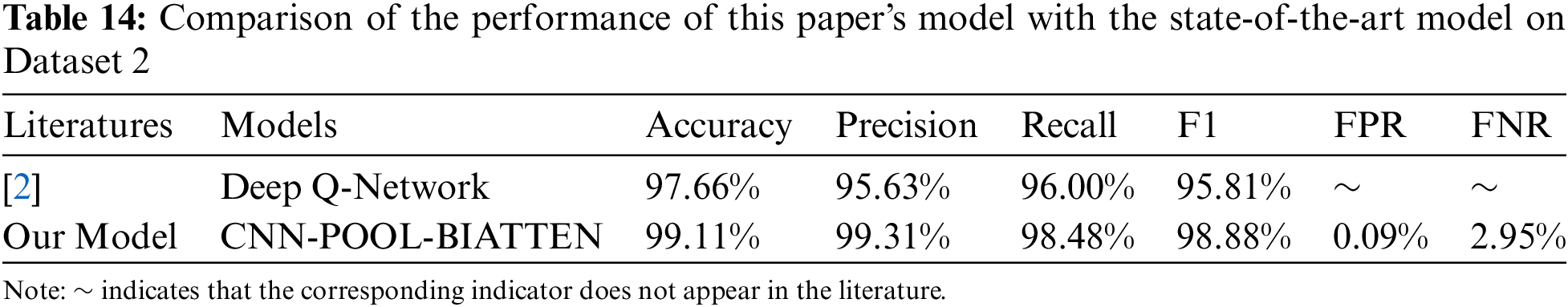
(2) Dataset 2

As shown in Table 14, on Dataset 2, the CNN-POOL-BIATTEN model outperforms the Deep Q-Network model of Thajeel et al. [2] in all metrics, particularly excelling in accuracy and precision rates, which are 99.11% and 99.31%, respectively. In contrast, Deep Q-Network has an accuracy of 97.66% and a precision of 95.63%, which are lower than those of the CNN-POOL-BIATTEN model. Although CNN-POOL-BIATTEN has a slightly higher miss rate of 2.95%, this discrepancy is within acceptable limits relative to its recall of 98.48% and F1 score of 98.88%. Thus overall, CNN-POOL-BIATTEN outperforms the Deep Q-Network model [2].

(3) Dataset 3

As shown in Table 15, in the performance evaluation of Dataset 3, we compare our CNN-POOL-BIATTEN model to the models reported in recent literature. Specifically, literature [26] describes how an improved Generative Adversarial Network (GAN) is used within an unsupervised deep learning approach to improve IoT attack detection performance, while literature [27] uses an integrated learning approach with a combination of four machine learning classifiers, while literature [28–31] includes the combination of bagging and Deep Neural Networks (DNN), support vector machines (SVMs), a hybrid model of KNN and SVMs, as well as state-of-the-art techniques for integrating Recursive Neural Network (ReNet), Transformer, and BiLSTM. All of these methods have been empirically tested on Dataset 3 to achieve high accuracy rates and represent the latest advances in the field. To better evaluate our model, we have compared the performance of these state-of-the-art models with that of our model.

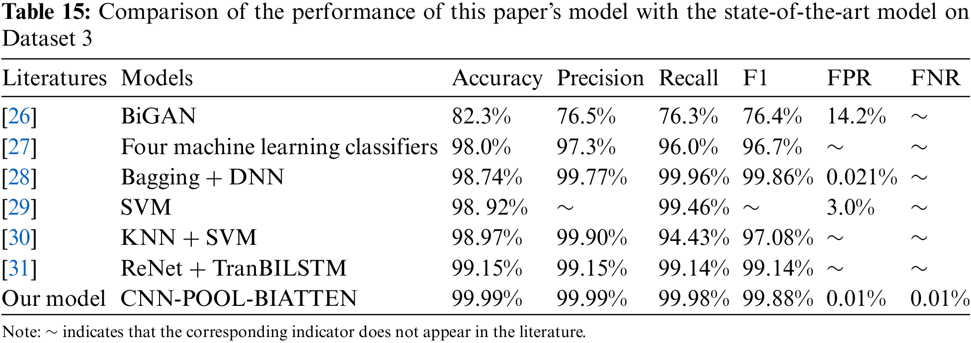
Comparison results show that the CNN-POOL-BIATTEN model achieves 99.99% accuracy, 99.99% precision, and 99.99% recall, with an F1 score of 99.88%. These values significantly surpass the 82.3% accuracy of the Bidirectional Generative Adversarial Network (BiGAN) model [26] and the 98.0% accuracy of the integrated model of four machine learning classifiers [27], indicating its superior ability to identify correct classifications and effectively reduce misclassifications. In comparison to the high performance of the Bagging + DNN model [28], CNN-POOL-BIATTEN still exhibits a slight advantage in these key metrics. Furthermore, even when comparing with efficient models such as SVM model [29] (98.92% accuracy, 99.46% precision) and KNN + SVM model [30] (98.97% accuracy, 99.90% precision, 94.43% recall), our model better balances recall while maintaining high precision. In comparison with the ReNet + TranBILSTM model [31], while the latter performs near-perfectly in terms of accuracy, precision, and recall (all 99.15%), our CNN-POOL-BIATTEN model continues to demonstrate a slight advantage in these performance metrics.

(4) Dataset 4

As shown in Table 16, in the performance evaluation of Dataset 4, we compare our CNN-POOL-BIATTEN model to a range of state-of-the-art models proposed in the literature. These models include SVMs, CNNs, CNN-BiLSTM, composite models that combine graph neural networks, self-attention mechanisms, and BiLSTMs, an innovative combination of LR and artificial bee colony algorithms, a combination of DTs and Random Forests, DNNs, Artificial Neural Networks (ANNs), a combination of KNNs and SVMs, and a combination of Bagging and DNNs. In addition, the literature includes a variety of integrated learning models such as Gradient Boosting Machine (GBM), Lightweight Gradient Boosting Machine (LGBM), XGBoost, and CatBoost. These studies employ diverse machine learning and deep learning methods, representing the state-of-the-art in the field of XSS, all of which have been experimentally validated on Dataset 4. To evaluate our model comprehensively, we analyze the performance of our model in comparison with the performance of models in the latest literature.

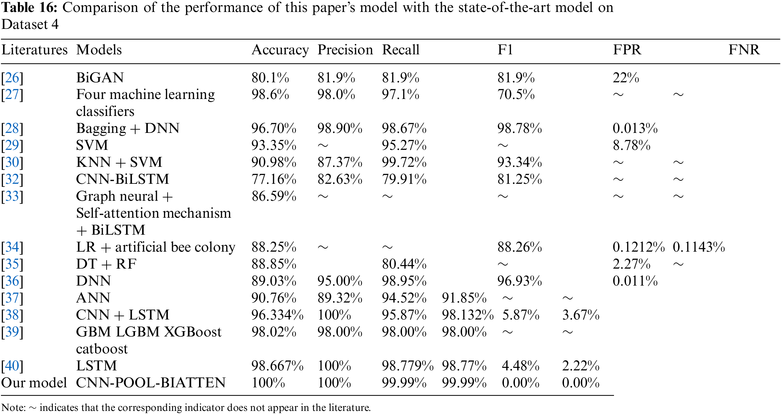
In the performance analysis of Dataset 4, while each of the other models has its own features and strengths, our CNN-POOL-BIATTEN model demonstrates certain advantages in key metrics. For example, when compared with models like CNN-BiLSTM [32] and BiGAN [26], the latter are effective but still fall short in accuracy, achieving 77.16% and 80.1% respectively, whereas our model achieves 100% accuracy. Similarly, the graph neural network combined with self-attention mechanism and BiLSTM model [33], as well as the model combining LR and artificial bee colony algorithms [34], although they made progress in accuracy, still fell short of our model. Even the models with better performance such as DT + RF model [35], DNN model [36], ANN model [37], KNN + SVM model [30], SVM model [29], and CNN+ LSTM [38], which have accuracies ranging from 88.85% to 96.334%, are still considerably inferior to the performance of our model. Although models like Bagging + DNN model [28], GBM (LGBM XGBoost, Catboost) model [39], and the four machine learning classifiers [27] perform well, our CNN-POOL-BIATTEN model has a slight advantage in accuracy, precision, and recall.

It is worth noting that although Kanna et al. and Sengur et al. employed the CNN + LSTM and LSTM models [38,40] respectively and both achieved 100% accuracy, these two approaches seem to have some limitations compared to our proposed CNN-POOL-BiLSTM model when other key performance metrics are considered together. Our model incorporates the properties of CNN and BiLSTM, effectively combining the advantages of CNN in detailed feature extraction and the capability of BiLSTM in capturing long-term dependencies. Additionally, by integrating the maximum pooling layer, our model is able to identify and highlight key features more effectively. Meanwhile, the introduced multi-attention mechanism further enhances the model’s ability in global feature representation, thereby demonstrating superior performance in several key performance metrics. This convergence of methodologies not only improves the generalisation ability of the model, but also provides new perspectives on feature extraction and analysis on complex datasets.

6  Conclusion

In this study, we have successfully developed an innovative model that combines Random Forest feature enhancement with the CNN-POOL-BIATTEN architecture, specifically designed to efficiently detect XSS attacks. The model achieves efficient feature extraction and data fusion through the integration of machine learning and deep learning techniques, significantly enhancing detection accuracy while effectively mitigating the risk of overfitting and false alarms. The originality of the model is manifested in its use of leaf node indexing from Random Forest as a key factor in expanding the feature set, combined with 1D convolutional layers, max 1D pooling layers, BiLSTM, and a multi-head attention mechanism, to thoroughly extract the local and global features of the data.

Through extensive validation across six public datasets, including comparisons with four traditional machine learning methods, comparative analysis with recent models from the past two years, and a series of detailed ablation experiments, the model demonstrates nearly perfect detection results, especially on the UNSW-NB15 and CICIDS2017 datasets, achieving 100% and 99.99% accuracy, respectively. This not only validates the model’s effectiveness, but also showcases its excellent performance and superior generalization capabilities across multiple datasets, thereby ensuring the model’s adaptability.

Additionally, by creating datasets specifically tailored for XSS attacks, this study further confirms the model’s effectiveness and utility in real-world applications, offering a novel and efficient solution for detecting XSS attacks in complex network environments and varied attack patterns. This work not only advances the application of machine learning and deep learning in network security but also introduces a new solution for future security protection against complex network environments and varied attack patterns.

7  Future Directions

In future studies, we aim to address the prevalent issue of data imbalance in datasets through the application of GANs. GANs have the potential to enhance the training dataset by generating synthetic data samples, particularly advantageous in categories with scarce samples, thus boosting the model’s capability to recognize various types of attacks. Concurrently, we recognize the challenges in model interpretability due to its complex architecture. We are currently investigating advanced interpretability techniques, including Local Interpretable Model-agnostic Explanations and Shapley Additive Explanations. Although these techniques are not implemented in the current model version, we plan to assess and incorporate these approaches in subsequent iterations. This strategy is expected to enhance the model’s transparency and interpretability, essential for addressing cybersecurity challenges and achieving an optimal balance between performance and interpretability.

Acknowledgement: Not applicable.

Funding Statement: The authors received no specific funding for this study.

Author Contributions: The authors confirm contribution to the paper as follows: study conception and design: Qiurong Qin, Yueqin Li; data collection: Yajie Mi; analysis and interpretation of results: Jinhui Shen; draft manuscript preparation: Kexin Wu, Zhenzhao Wang. All authors reviewed the results and approved the final version of the manuscript.

Availability of Data and Materials: Data will be made available on request.

Conflicts of Interest: The authors declare that they have no conflicts of interest to report regarding the present study.

References

1. C. Liu, X. Cui, Z. Wang, X. Wang, Y. Feng and X. Li, “Malicescript: A novel browser-based intranet threat,” in 2018 IEEE Third Int. Conf. Data Sci. Cyberspace (DSC), Guangzhou, China, IEEE, 2018, pp. 219–226. [Google Scholar]

2. I. K. Thajeel, K. Samsudin, S. J. Hashim, and F. Hashim, “Dynamic feature selection model for adaptive cross site scripting attack detection using developed multi-agent deep Q learning model,” J. King Saud Univ.-Comput. Inf. Sci., vol. 35, no. 6, pp. 101490, 2023. [Google Scholar]

3. U. Sarmah, D. Bhattacharyya, and J. K. Kalita, “A survey of detection methods for XSS attacks,” J. Netw. Comput. Appl., vol. 118, no. 2–3, pp. 113–143, 2018. doi: 10.1016/j.jnca.2018.06.004. [Google Scholar] [CrossRef]

4. V. Nithya, S. L. Pandian, and C. Malarvizhi, “A survey on detection and prevention of cross-site scripting attack,” Int. J. Secur. Appl., vol. 9, no. 3, pp. 139–152, 2015. doi: 10.14257/ijsia.2015.9.3.14. [Google Scholar] [CrossRef]

5. B. B. Gupta and P. Chaudhary, Cross-Site Scripting Attacks: Classification, Attack, and Countermeasures. Boca Raton: CRC Press, 2020. [Google Scholar]

6. G. E. Rodríguez, J. G. Torres, P. Flores, and D. E. Benavides, “Cross-site scripting (XSS) attacks and mitigation: A survey,” Comput. Netw., vol. 166, no. 4, pp. 106960, 2020. doi: 10.1016/j.comnet.2019.106960. [Google Scholar] [CrossRef]

7. J. Howe and F. Mereani, “Detecting cross-site scripting attacks using machine learning,” Adv. Intell. Syst. Comput., vol. 723, pp. 200–210, 2018. [Google Scholar]

8. M. Liu, B. Zhang, W. Chen, and X. Zhang, “A survey of exploitation and detection methods of XSS vulnerabilities,” IEEE Access, vol. 7, pp. 182004–182016, 2019. doi: 10.1109/ACCESS.2019.2960449. [Google Scholar] [CrossRef]

9. T. Hu, C. Xu, S. Zhang, S. Tao, and L. Li, “Cross-site scripting detection with two-channel feature fusion embedded in self-attention mechanism,” Comput. Secur., vol. 124, no. 12, pp. 102990, 2023. doi: 10.1016/j.cose.2022.102990. [Google Scholar] [CrossRef]

10. X. Chen, M. Li, Y. Jiang, and Y. Sun, “A comparison of machine learning algorithms for detecting XSS attacks,” in Artif. Intell. Secur.: 5th Int. Conf., ICAIS 2019, New York, NY, USA, Springer, 2019, pp. 214–224. [Google Scholar]

11. R. Wang, X. Jia, Q. Li, and S. Zhang, “Machine learning based cross-site scripting detection in online social network,” in 2014 IEEE Intl. Conf. High Performance Comput. Commun., 2014 IEEE 6th Intl. Symp. Cyberspace Safety Secur., 2014 IEEE 11th Intl. Conf. Embedded Softw. Syst., Paris, France, IEEE, 2014, pp. 823–826. [Google Scholar]

12. G. Habibi and N. Surantha, “XSS attack detection with machine learning and n-gram methods,” in 2020 Int. Conf. Inf. Manag. Technol. (ICIMTech), Bandung, Indonesia, IEEE, 2020, pp. 516–520. [Google Scholar]

13. S. Rathore, P. K. Sharma, and J. H. Park, “XSSClassifier: An efficient XSS attack detection approach based on machine learning classifier on SNSs,” J. Inf. Process. Syst., vol. 13, no. 4, 2017. doi: 10.3745/JIPS.03.0079. [Google Scholar] [CrossRef]

14. Y. Fang, Y. Li, L. Liu, and C. Huang, “DeepXSS: Cross site scripting detection based on deep learning,” in Proc. 2018 Int. Conf. Comput. Artif. Intell., New York, NY, USA, 2018, pp. 47–51. [Google Scholar]

15. Z. Liu, Y. Fang, C. Huang, and J. Han, “GraphXSS: An efficient XSS payload detection approach based on graph convolutional network,” Comput. Secur., vol. 114, no. 3, pp. 102597, 2022. doi: 10.1016/j.cose.2021.102597. [Google Scholar] [CrossRef]

16. F. M. M. Mokbal, W. Dan, X. X. Wang, W. B. Zhao, and L. H. Fu, “XGBXSS: An extreme gradient boosting detection framework for cross-site scripting attacks based on hybrid feature selection approach and parameters optimization,” J. Inf. Secur. Appl., vol. 58, pp. 102813, 2021. doi: 10.1016/j.jisa.2021.102813. [Google Scholar] [CrossRef]

17. C. Li, Y. Wang, C. Miao, and C. Huang, “Cross-site scripting guardian: A static XSS detector based on data stream input-output association mining,” Appl. Sci., vol. 10, no. 14, pp. 4740, 2020. doi: 10.3390/app10144740. [Google Scholar] [CrossRef]

18. S. Abaimov and G. Bianchi, “CODDLE: Code-injection detection with deep learning,” IEEE Access, vol. 7, pp. 128617–128627, 2019. doi: 10.1109/ACCESS.2019.2939870. [Google Scholar] [CrossRef]

19. J. R. Tadhani, V. Vekariya, V. Sorathiya, S. Alshathri, and W. El-Shafai, “Securing web applications against XSS and SQLi attacks using a novel deep learning approach,” Sci. Rep., vol. 14, no. 1, pp. 1803, 2024. doi: 10.1038/s41598-023-48845-4. [Google Scholar] [PubMed] [CrossRef]

20. A. A. Farea et al., “Injections attacks efficient and secure techniques based on bidirectional long short time memory model,” Comput. Mater. Contin., vol. 76, no. 3, pp. 3605–3622, 2023. doi: 10.32604/cmc.2023.040121 [Google Scholar] [CrossRef]

21. F. M. M. Mokbal, W. Dan, A. Imran, J. C. Lin, F. Akhtar and X. X. Wang, “MLPXSS: An integrated XSS-based attack detection scheme in web applications using multilayer perceptron technique,” IEEE Access, vol. 7, pp. 100567–100580, 2019. doi: 10.1109/ACCESS.2019.2927417. [Google Scholar] [CrossRef]

22. I. Sharafaldin, A. H. Lashkari, and A. A. Ghorbani, “Toward generating a new intrusion detection dataset and intrusion traffic characterization,” in ICISSP, vol. 1, pp. 108–116, 2018. doi: 10.5220/0006639801080116. [Google Scholar] [CrossRef]

23. I. Sharafaldin, A. Gharib, A. H. Lashkari, and A. A. Ghorbani, “Towards a reliable intrusion detection benchmark dataset,” Softw. Netw., vol. 2018, no. 1, pp. 177–200, 2018. doi: 10.13052/jsn2445-9739.2017.009. [Google Scholar] [CrossRef]

24. N. Moustafa and J. Slay, “UNSW-NB15: A comprehensive data set for network intrusion detection systems (UNSW-NB15 network data set),” in 2015 Military Commun. Inf. Syst. Conf. (MilCIS), IEEE, 2015, pp. 1–6. [Google Scholar]

25. M. Tavallaee, E. Bagheri, W. Lu, and A. A. Ghorbani, “NSL-KDD dataset,” vol. 114, 2012. Accessed: 28 Feb. 2016. [Online]. Available: http://www.unb.ca/research/iscx/dataset/iscx-NSL-KDD-dataset.html [Google Scholar]

26. W. Yao, H. Shi, and H. Zhao, “Scalable anomaly-based intrusion detection for secure internet of things using generative adversarial networks in fog environment,” J. Netw. Comput. Appl., vol. 214, no. 11, pp. 103622, 2023. doi: 10.1016/j.jnca.2023.103622. [Google Scholar] [CrossRef]

27. M. A. Khan, N. Iqbal, H. Jamil, and D. H. Kim, “An optimized ensemble prediction model using AutoML based on soft voting classifier for network intrusion detection,” J. Netw. Comput. Appl., vol. 212, no. 3, pp. 103560, 2023. doi: 10.1016/j.jnca.2022.103560. [Google Scholar] [CrossRef]

28. A. Thakkar and R. Lohiya, “Attack classification of imbalanced intrusion data for IoT network using ensemble learning-based deep neural network,” IEEE Internet Things J., vol. 10, no. 13, pp. 11888–11895, 2023. doi: 10.1109/JIOT.2023.3244810. [Google Scholar] [CrossRef]

29. J. Gu and S. Lu, “An effective intrusion detection approach using SVM with Naïve Bayes feature embedding,” Comput. Secur., vol. 103, no. 3, pp. 102158, 2021. doi: 10.1016/j.cose.2020.102158. [Google Scholar] [CrossRef]

30. M. Yousefnezhad, J. Hamidzadeh, and M. Aliannejadi, “Ensemble classification for intrusion detection via feature extraction based on deep learning,” Soft Comput., vol. 25, no. 20, pp. 12667–12683, 2021. doi: 10.1007/s00500-021-06067-8. [Google Scholar] [CrossRef]

31. S. Wang, W. Xu, and Y. Liu, “Res-TranBiLSTM: An intelligent approach for intrusion detection in the internet of things,” Comput. Netw., vol. 235, pp. 109982, 2023. doi: 10.1016/j.comnet.2023.109982. [Google Scholar] [CrossRef]

32. K. Jiang, W. Wang, A. Wang, and H. Wu, “Network intrusion detection combined hybrid sampling with deep hierarchical network,” IEEE Access, vol. 8, pp. 32464–32476, 2020. doi: 10.1109/ACCESS.2020.2973730. [Google Scholar] [CrossRef]

33. X. Wang, X. Wang, M. He, M. Zhang, and Z. Lu, “Spatial-temporal graph model based on attention mechanism for anomalous IoT intrusion detection,” IEEE Trans. Ind. Inform., vol. 99, pp. 1–3, 2023. doi: 10.1109/TII.2023.3308784. [Google Scholar] [CrossRef]

34. B. Kolukisa, B. K. Dedeturk, H. Hacilar, and V. C. Gungor, “An efficient network intrusion detection approach based on logistic regression model and parallel artificial bee colony algorithm,” Comput. Stand. Inter., vol. 89, pp. 103808, 2023. [Google Scholar]

35. H. Zhang, J. L. Li, X. M. Liu, and C. Dong, “Multi-dimensional feature fusion and stacking ensemble mechanism for network intrusion detection,” Future Gener. Comput. Syst., vol. 122, pp. 130–143, 2021. doi: 10.1016/j.future.2021.03.024. [Google Scholar] [CrossRef]

36. A. Thakkar and R. Lohiya, “Fusion of statistical importance for feature selection in deep neural network-based intrusion detection system,” Inf. Fusion, vol. 90, no. 1, pp. 353–363, 2023. doi: 10.1016/j.inffus.2022.09.026. [Google Scholar] [CrossRef]

37. M. Rani, Gagandeep, “Effective network intrusion detection by addressing class imbalance with deep neural networks multimedia tools and applications,” Multimed. Tools Appl., vol. 81, no. 6, pp. 8499–8518, 2022. doi: 10.1007/s11042-021-11747-6. [Google Scholar] [CrossRef]

38. P. R. Kanna and P. Santhi, “Unified deep learning approach for efficient intrusion detection system using integrated spatial-temporal features,” Knowl. Based Syst., vol. 226, no. 1, pp. 107132, 2021. doi: 10.1016/j.knosys.2021.107132. [Google Scholar] [CrossRef]

39. I. F. Kilincer, F. Ertam, and A. Sengur, “A comprehensive intrusion detection framework using boosting algorithms,” Comput. Electr. Eng., vol. 100, pp. 107869, 2022. doi: 10.1016/j.compeleceng.2022.107869. [Google Scholar] [CrossRef]

40. P. R. Kanna and P. Santhi, “Hybrid intrusion detection using mapreduce based black widow optimized convolutional long short-term memory neural networks,” Expert Syst. Appl., vol. 194, no. 9, pp. 116545, 2022. doi: 10.1016/j.eswa.2022.116545. [Google Scholar] [CrossRef]