Evolutionary Variational YOLOv8 Network for Fault Detection in Wind Turbines

1  Introduction

The continuous expansion of wind power and the aging of wind turbines underscore the critical importance of extending the service life of wind turbine blades. Effective maintenance and prompt fault detection are paramount for the optimal operation of wind farms and the enhancement of power generation efficiency [1]. Wind turbine blades (WTBs), which are centered on the wind turbine, are subjected to high loads and harsh environmental conditions, making them vulnerable to defects such as gel coat erosion and paint peeling, which can adversely affect power generation efficiency and safety [2]. Therefore, early and accurate detection of surface defects on WTBs is crucial.

Traditional methods for detecting WTBs defects rely on visual inspections and sensor monitoring, which have their drawbacks. For instance, the use of fiber optic sensors, while innovative, incurs high costs and logistical challenges. Similarly, the guided wave ultrasound air coupling technique, though capable of identifying defect dimensions, struggles with weak signals obscured by noise. These methods lack specificity in identifying defect types. Machine learning (ML) offers new avenues for defect detection in WTBs. Nick et al. [3] proposed an unsupervised learning method to discern both the existence and the specific locations of damage through acoustic emission signals. This method was then enhanced by adopting supervised learning for a detailed analysis of fault types and their severities. Although these techniques excel in fault identification and exhibit resilience against overfitting, they fall short in achieving optimal detection outcomes and display limited robustness amidst the challenging conditions presented by wind energy sites. Deng et al. [4] developed an adaptive filtering approach, integrating an enhanced LPSO algorithm with a log-Gabor filter and employing a classifier to categorize defects in images of WTBs effectively, thereby facilitating accurate defect feature extraction. Nonetheless, the efficacy of feature extraction is compromised by the variability in filter orientation and bandwidth, potentially leading to misclassification and extended processing durations. These challenges underscore the urgent necessity for devising more effective and alternative strategies for fault detection in WTBs. Utilizing an acoustic emission system, Wei et al. [5] proposed a range of faults in WTBs despite its proficiency in real-time monitoring of acoustic emissions to fault detection, this method is susceptible to false positives, mistakenly identifying extraneous signals as fault indicators and generating misleading noise. Additionally, the detection process carries a risk of inflicting damage on the blades themselves. These limitations emphasize the imperative for more accurate and harmless fault detection methodologies in WTBs.

With developments in computer vision (CV) technology, DL has emerged as a promising solution [6–8]. This technology excels in processing large datasets, thereby enhancing detection efficiency and accuracy through DL algorithms. It enables the identification of complex defect patterns without physical contact, reducing potential damage and safety risks. Moreover, DL-based CV offers scalability, adaptability, and automation, facilitating continuous optimization and requiring minimal manual intervention. Thus, it represents a comprehensive solution for efficient, accurate, and safe fault detection in wind turbine blades. The advent of region-based convolutional neural networks (CNNs) and innovations such as the You Only Look Once (YOLO) series have revolutionized target detection and recognition in DL [9]. Currently, the YOLOv5 algorithm demonstrates high accuracy and rapid detection speeds, proving effective in various applications [10]. Despite the emergence of newer versions, YOLOv5 remains a preferred choice for specific detection tasks due to its balance of speed and accuracy.

Recently, neural architecture search (NAS) employs a system of automated exploration to forge network designs tailored to the specific demands of various tasks, achieving significant advancements across numerous practical applications, including image segmentation, smart conversation systems, and semantic identification [11]. The existing methodologies within this field are generally categorized into three distinct types based on their underlying search strategies. Reinforcement learning (RL)-based methods aim to develop high-efficiency models through the extensive training of controllers, a process that proves to be both time-intensive and impractical for devices with limited computational resources [12]. Meanwhile, gradient-based strategies utilize the backpropagation of clearly defined mathematical formulations for evaluating the significance of different architectures, though this approach requires the preliminary construction of a comprehensive supernet [13]. On the other hand, approaches grounded in evolutionary computation (EC) propel the identification of the most suitable architecture by leveraging a generative process across a population of potential designs [14]. Comparative experiments have consistently demonstrated that the performance and efficiency of EC-based methods surpass those reliant on RL, indicating a promising direction for future NAS endeavors.

Compared to previous works, this work has the advantage of addressing several limitations, including: 1) Fault detection methods often impose constraints on the maximum depth of the network, impeding the exploration of optimal architectures for diverse tasks; 2) The network model tends to be oversized, posing challenges for deployment on resource-constrained devices like smartwatches. 3) NAS is typically resource-intensive, making the attainment of an ideal architecture costly, often requiring the utilization of hundreds of GPUs. This work introduces an evolutionary variational YOLOv8 network method for fault detection (EV-YOLOv8), aiming to overcome the limitations of previous models and further enhance the accuracy and efficiency of WTB fault detection. Accordingly, the main contributions of this work include:

1.    Addressing the issue of extensive manual effort required for hyperparameter tuning, this paper introduces a method of flexible variable-length encoding along with specially designed reproduction operators. These innovations facilitate the identification of optimal hyperparameter settings, effectively reducing the manual workload involved in model configuration.

2.    It integrates the FasterNet module, which uses PConv as its core operator, into the cross-stage partial Darknet-53 framework to create an advanced feature extraction network. This newly formulated network serves as the backbone for the EV-YOLOv8 method, aiming to streamline the model by reducing the number of parameters, and simplifying network architecture.

3.    To mitigate potential reductions in detection accuracy due to the modifications in the backbone network, the research employs the EfficicCIoU loss function. This innovative loss function merges the principles of efficient complete intersection over union with complete intersection over union, promoting quicker convergence and thereby improving detection precision.

4.    Experimental results confirm that our method can achieve better fault detection results and improve by 2.6% in mean precision at 50 compared to the existing methods. Additionally, compared to training with the YOLOv8 model, the EV-YOLOv8 model reduces the training parameters by 933,937 and decreases GFLOPS by 1.1.

The rest of this work is organized as follows. Section 2 briefly reviews CNNs for fault detection, YOLO series methods, and neural architecture search. Section 3 delves into the challenges related to the excessive number of parameters and the complexity of the network observed during the training of the YOLOv8 model. Section 4 is devoted to experimental studies and analysis. This section details the construction of a proprietary dataset and the parameter configurations employed. Finally, the conclusions and the future directions are displayed in Section 5.

2  Related Work

2.1 Convolutional Neural Networks

Girshick et al. [15] introduced R-CNN, a two-stage object detection algorithm utilizing CNNs to generate candidate regions, extract features via CNN, classify these features with an SVM, and refine object positions with a regressor. Although revolutionary, R-CNN’s selective search for candidate regions slows it down, and processing each region through CNN adds computational redundancy. However, this approach strains CNN’s training efficiency due to larger receptive fields. Microsoft Research’s Fast R-CNN addressed these issues by incorporating an ROI pooling layer and a multi-task loss function, optimizing the cropping and scaling process but still relying on selective search for region generation, indicating potential areas for further improvements [16]. Guo et al. [17] developed a multi-level identification system for WTBs that incorporates a Haar-AdaBoost method for suggesting regions and a convolutional neural network classifier to detect damage and diagnose faults. Cheng et al. [18] proposed a temporal attention-based CNN to evaluate the risk of WTB icing.

2.2 YOLO-Based Algorithms

Redmon et al. [9] introduced YOLOv1, an end-to-end deep learning solution for object detection that predicts object classes and locations directly, significantly speeding up detection without needing candidate regions. Despite its speed, YOLOv1 struggled with detecting small, densely packed objects due to bounding box limitations. YOLOv2 improved versatility with the Darknet-19 network, joint dataset training, hierarchical classification, and more classification data. However, its use of anchor boxes slightly reduced accuracy [19]. YOLOv3 balanced speed and accuracy with the Darknet-53 architecture and altered box classification methods [20]. YOLOv4 boosted performance by integrating cross-stage partial connections to simplify the model [21]. The series advanced with YOLOv5, focusing on user accessibility and deployment, and YOLOv6s, which featured the EfficientRep model and a novel loss function [22]. YOLOv7 introduced a scalable network for model concatenation, while the latest YOLOv8 streamlined its backbone with CSPDarknet-53 and a C2F module, leading to a larger model requiring significant computational resources [23,24]. Yao et al. [25] proposed a lightweight cascaded feature fusion neural network model based on YOLOX for detecting damage to WTBs. Zhang et al. [26] introduced a high-accuracy model, SOD-YOLO, for detecting surface defects on WTBs utilizing image analysis from unmanned aerial vehicles based on YOLOv5 technology.

2.3 Neural Architecture Search

NAS is expected to fast-track the discovery of neural networks tailored to specific datasets [27,28]. Current methods fall into three categories: RL, Gradient-based, and EC. RL methods use an RNN to create designs, using validation performance for feedback to refine training, with RL hyperparameter choices critically affecting efficiency [12]. Gradient-based approaches speed up optimization by incorporating operation choices directly, though they can be unstable. EC strategies, growing in popularity, use fitness functions for evolutionary solution development, advantageous for their gradient independence and less hyperparameter sensitivity [14]. This shift towards EC highlights its effectiveness in overcoming NAS optimization challenges. For example, a novel method that employs a multi-objective evolutionary algorithm, integrating a probability stack, tailored for NAS [29]. The method aims to optimize both accuracy and computational efficiency. Moreover, an innovative NAS technique that utilizes an adaptive, scalable framework [30]. This is achieved through the application of a reinforcement-based I-Ching divination evolutionary algorithm, alongside a flexible architecture encoding strategy.

Efficiency in NAS is hampered by the high computational cost of evaluating new architectures. For example, the first NAS project consumed over 800 GPUs for 28 days to find an optimal CNN design [12]. To address this, several strategies have been introduced: early stopping quickly gauges architecture performance with minimal training [31]; performance prediction uses surrogate models trained on known outcomes to estimate new architectures’ efficacy [32]; and weight inheritance allows architectures to use pre-trained model weights, speeding up evaluation [33]. Among weight inheritance methods, Supernet and population memory are notable, with the latter specifically preventing redundant evaluations in EC-based NAS by reusing outcomes from previous generations, thus saving computational resources [34].

2.4 Evolutionary Computation

EC utilizes a search methodology inspired by natural selection, designed to address a variety of optimization problems (such as discrete, dynamic, and multi-objective optimization) through the adoption of mechanisms derived from biological processes, including crossover, mutation, and selection based on environmental pressures [35–38]. The structure of a standard EC system is outlined as follows: Initialization involves utilizing a predetermined encoding method to depict a population of individuals. During the Evaluation phase, each individual’s fitness level is assessed. In the reproduction step, offspring are produced from the parental population using a series of reproductive mechanisms. In environmental selection, the fitness levels of the offspring are evaluated and merged with those of the parents to form a new generation, prioritizing individuals based on their fitness. The process then loops back to reproduction, continuing until a specific termination criteria, such as reaching a maximum number of generations set by the user, is met. Sessarego et al. [39] combined multi-objective evolutionary algorithm (MOEA) with gradient based local search and concluded that compared to traditional MOEA, optimal blade design can be achieved at lower computational costs. Jakub et al. [40] proposed a evolutionary computing algorithm for small wind turbine supporting structures.

3  Method

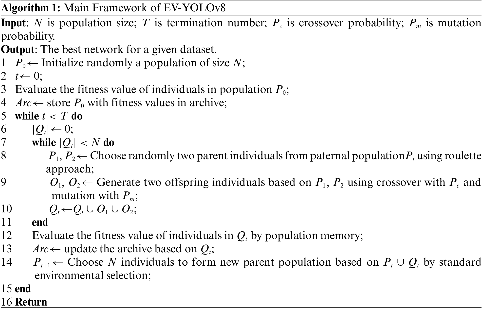
3.1 NAS-Based Optimization for YOLOv8

In the training process of advanced YOLOv8 model, it is crucial to make reasonable choices and optimize hyperparameters. Different combinations of hyperparameters can result in significant differences in training outcomes. An optimal hyperparameter configuration can maximize the performance of the model, especially in terms of accuracy and efficiency. However, due to the vastness and diversity of the hyperparameter space, as well as the complex interactions that may exist between different hyperparameters. Manually adjusting hyperparameters is both time-consuming and difficult to guarantee finding the global optimal solution. In previous hyperparameter tuning tasks, manual adjustment methods are commonly used, but manually adjusting hyperparameters is both time-consuming and difficult to guarantee finding the global optimal solution. To effectively address this problem, this paper proposes the NAS-based hyperparameter optimization method to achieve effective optimization of hyperparameters in YOLOv8 algorithm training. Specifically, the framework of EV-YOLOv8 is provided in Algorithm 1.

3.1.1 Initialization

Each individual in our method undergoes an initialization process based on a recommended encoding strategy, where each encoding represents a potential architecture for a CNN. To boost the flexibility of these architectures, we introduce a scheme of variable length encoding that is capable. of depicting networks with various depths. This innovative encoding strategy thus allows for the accommodation of network architectures featuring a range of depths, enhancing the model’s adaptability. The structure of our architectural designs is influenced by the notable successes of ResNet, DenseNet, and MobileNet-v2, incorporating Residual Blocks (RB), Dense Blocks (DB), Mobile Blocks (MB), and pooling operations, as shown in Fig. 1. Our main attention is directed towards the management of input and output channel numbers. The convolutional operations within the RB, DB, and MB units are held constant. For pooling operations, our focus is on their types, such as max and mean pooling, making up the architecture’s RB units (RBU), DB units (DBU), MB units (MBU), and pooling units (PU). Each of these units—RBU, DBU, and MBU—comprises multiple RB, DB, and MB units, respectively, while the PU includes a single pooling operation. To aid in algorithmic processes, two additional parameters indicate the unit’s position and type.

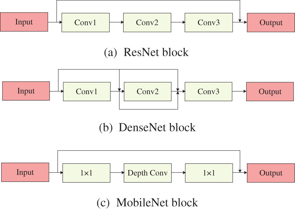
Figure 1: Three classical block CNNs

A visual representation of our encoding scheme is provided, detailing five key units. The numerical values displayed within a gray rectangle illustrate the unit’s position within the CNN’s structure. The type values—1 for RBU, 2 for DBU, 3 for MBU, and 4 for PU—define the unit type. Additionally, the letters A, I, and O represent the number of units, input channel count, and output channel count, respectively. Several constraints are applied to ensure architectural coherence: The input channel count of the first unit must match that of the input data, the first unit cannot be a PU, and the input channel count for any subsequent unit must equal the output channel count of its predecessor, ensuring seamless connectivity within the architecture.

3.1.2 Evaluation and Reproduction

Evaluation: To facilitate the environmental selection phase, we assess fitness based primarily on the accuracy of CNN. However, the determination of CNN accuracy is inherently time-consuming due to the extensive learning required for a large set of parameters through gradient-based methods. To reduce this computational burden, we have implemented a population memory strategy, anchored on a metric of similarity, that effectively utilizes the data from previously assessed architectures within the evolutionary search process. After the initial phase, each individual is evaluated to determine its baseline accuracy by training from scratch. Architectures that have been trained and their accuracies determined are then stored in an archive. When new offspring are generated, they are compared to the archived individuals based on their encoded architecture data. Should the degree of similarity between a new individual and any within the archive exceed a set threshold, the archived individual’s accuracy is adopted as the fitness value for the new offspring. In scenarios where more than one archived architecture meets the similarity criterion, the fitness value is derived from the one exhibiting the highest degree of similarity.

In instances where the similarity does not meet the threshold, the new individual’s accuracy is ascertained through the process of training from scratch, and upon obtaining this accuracy, the individual is added to the archive. For the purpose of assessing similarity, we employ cosine similarity as our metric of choice. This approach streamlines the evaluation process by avoiding redundant computations for architectures that are significantly similar to those already explored, thereby optimizing the overall efficiency of the evolutionary search.

S=AQ×AM|AQ|⋅|AM|(1)

where, AQ represents the offspring architecture’s encoding, and AM signifies the encoding of a previously archived architecture. The use of a flexible encoding method means encoding lengths can differ across architectures. To manage this variability and ease similarity calculation, shorter encodings are zero-padded to match the length of longer ones, ensuring consistent and accurate comparisons.

Using zero padding to streamline similarity assessments is essential for maintaining the efficiency of the evolutionary search process. It facilitates direct comparisons between newly generated offspring and existing architectures in the archive, despite differences in initial encoding lengths. This method efficiently identifies architectures similar to those previously evaluated, sparing them from the computationally demanding process of training from scratch. As a result, architectures that closely match archived ones, based on a predefined similarity threshold, avoid the extensive training process. Instead, their fitness values are directly derived from corresponding matches in the archive. This approach significantly speeds up the evolutionary search, optimizes the use of computational resources, and focuses efforts on exploring new and unique architectures.

Reproduction: In our local search process within the encoding space, the exchange of information between two parent solutions is a critical step. Due to the variable lengths of individuals within our population, caused by our flexible encoding scheme, traditional crossover methods do not suit our needs. As a solution, we employ a one-point crossover technique, which entails: Independently selecting a crossover point for each parent, which marks the position at which information exchange begins. Exchanging segments of the parents’ encodings past these crossover points, leading to the creation of offspring that combine characteristics from both parents. Making necessary adjustments to the offspring’s encoding to ensure compliance with predefined architectural constraints.

Regarding mutations, we implement three distinct operations: addition, deletion, and modification, each tailored to introduce variability and exploration within the architecture space. This mutation involves the random generation of a new unit (e.g., an MBU) and its subsequent insertion into a randomly selected position within the parent architecture. This step introduces new architectural features and is followed by adjustments to ensure the offspring adheres to the constraints. Addition: This mutation involves the random generation of a new unit (e.g., an MBU) and its subsequent insertion into a randomly selected position within the parent architecture. This step introduces new architectural features and is followed by adjustments to ensure the offspring adheres to the constraints. Deletion: In this operation, a unit is randomly selected for removal from the architecture. Once removed, the offspring architecture is restructured, and necessary adjustments are made to align with the constraints, possibly simplifying or refining the architecture. Modification: This process involves changing the details within a unit, such as its type, the number of units, and the input and output channel counts. The aim is to fine-tune the architectural characteristics without drastically altering its overall structure.

Each of these mutation operations plays a role in the evolutionary process, allowing for the exploration of the architectural space and the discovery of effective neural network designs. These strategies ensure that our search mechanism remains flexible and capable of navigating the complex landscape of possible network architectures.

3.2 FasterNet

To boost neural network model transmission speed and lower computational complexity, methods like depthwise convolution (DWConv) and graph convolution (Gconv) reduce Floating Point Operations (FLOPs) during feature extraction. However, these methods often increase memory access frequency, meaning FLOP reductions do not always translate to lower computational latency. This discrepancy, as outlined in Eq. (2), stems from the relatively low value of floating point operations per second (FLOPS), where Latency quantifies the latency calculation time.

Latency=FLOPsFLOPS(2)

The phenomenon where frequent memory access by the operator reduces FLOPs but does not equivalently reduce computing latency is clearly demonstrated with depthwise separable convolution (DWSConv). In DWSConv, the process is split into two steps: depthwise convolution (DWConv) and pointwise convolution (PWConv). DWConv processes each channel independently to preserve channel count, and though it lowers FLOPs, it can decrease detection accuracy. To mitigate this, PWConv follows DWConv, using varied kernel sizes to blend and reorganize the output channels, as specified in Eq. (3). This strategy efficiently balances computational cost and maintains performance.

P=h×w×k2×c(3)

where, P represents the number of parameters required for the convolution operation. h and w represent width and height of the feature map. k represents the size of the convolutional kernel, and c represents the number of channels used in the convolution operation.

The steps to construct FasterNet are shown below and the FasterNet block is shown in Fig. 2.

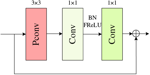
Figure 2: FasterNet block

Step 1: to sustain a high FLOPS ratio despite a reduction in FLOPs, the initial step involves integrating the FasterNet module, equipped with the Partial Convolution (PConv) operator, into the CSPDarknet-53 backbone network [41]. Step 2: the definition of the FasterNet block class is based on the PConv module, thereby establishing the structural foundation for the FasterNet block module. Step 3: the implementation of the forward propagation mechanism within the FasterNet block is achieved by defining the forward method. This process involves convolution of the input, optionally incorporating residual connections, and then summing this convolved output with the original input before yielding the convolution’s result. Step 4: the construction of the FasterNet architecture, utilizing the FasterNet block module, marks the subsequent step. This architecture is distinguished by comprising multiple FasterNet block, with the FasterNet constructor accepting parameters c1 and c2 to denote the count of input and output channels, respectively, and n to indicate the number of FasterNet block units. Step 5: the construction process culminates with the initialization of a Conv instance within the FasterNet constructor, completing the architectural setup for enhanced neural network performance.

3.3 CSPDarknet-53 Backbone Network

The improved backbone network architecture is shown in Table 1.

The image processing begins with two initial convolutional layers. The first layer uses 64 kernels to halve the input image size using a stride of 2, while the second layer employs 128 kernels to quarter the original image size. Feature extraction is then enhanced by the C2f module, performing three rounds of 128-kernel convolutions and activations. A third layer, using 256 kernels, further reduces the feature map size to one-eighth of the input. This is intensified by six cycles of 256-kernel convolutions in the C2f module. The fourth layer deepens the reduction, employing 512 kernels to shrink the feature map to one-sixteenth of the original size, augmented by six cycles of the FasterNet module. The process concludes with a fifth layer using 4 filters, ultimately reducing the feature map to one-thirty-second of the input. This efficient methodology ensures substantial feature map compression and refined feature extraction.

This refinement clarifies the sequential process of convolutional operations and feature extraction, emphasizing the methodical reduction of feature map sizes and the specific use of convolutional kernels and modules to enhance the extracted features. And, the feature extraction process using the FasterNet module is as follows: Firstly, we apply the FasterNet module three times consecutively to the feature maps for feature extraction. And each FasterNet module consists of a convolutional operation and an activation function and the convolutional operation uses 1024 convolution kernels. Then, we adopt the CSPDarknet-53 backbone network with the FasterNet module as the backbone network for the EV-YOLOv8 network model. The overall structure of the EV-YOLOv8 network model is shown in Fig. 3.

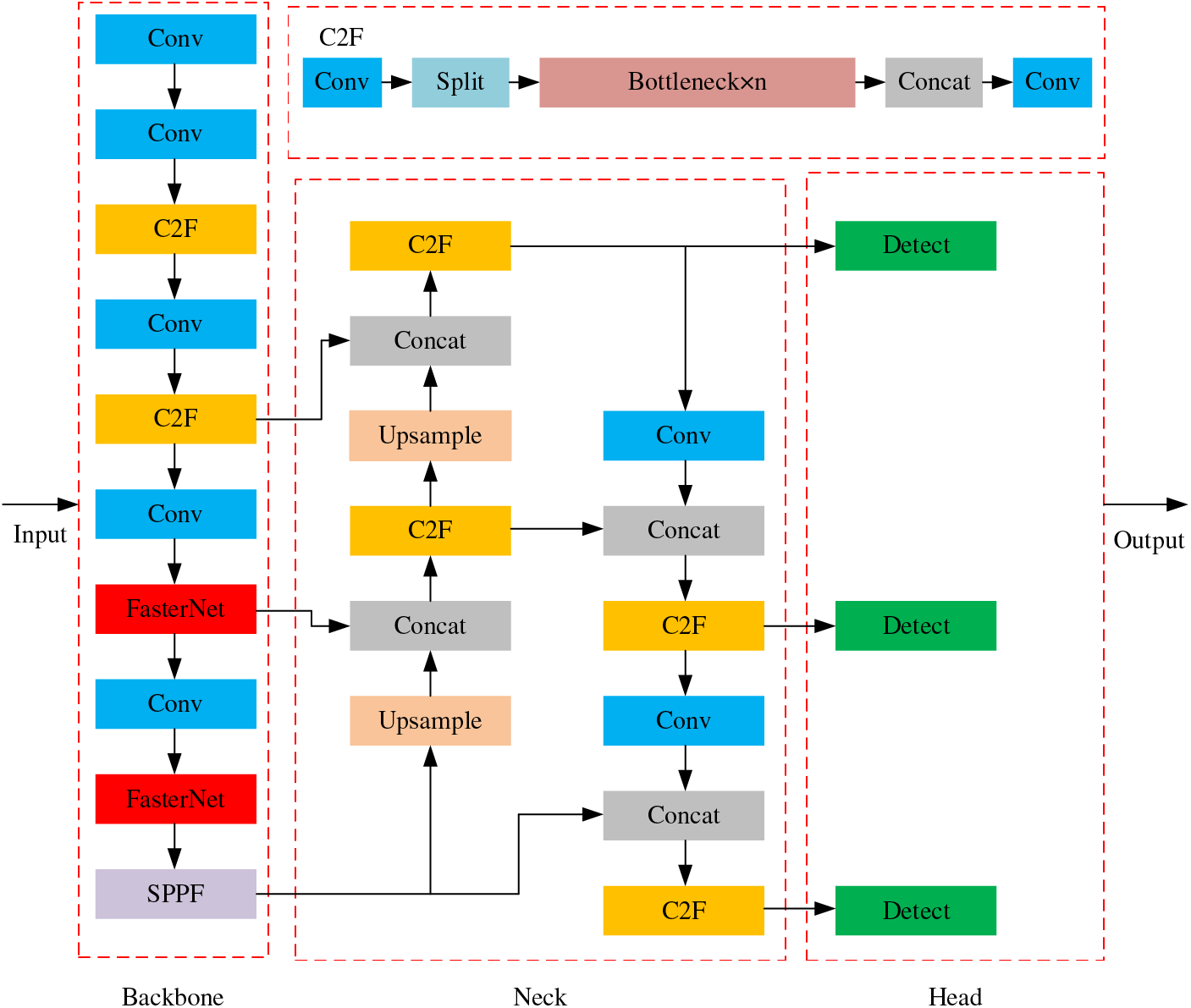
Figure 3: The network structure of EV-YOLOv8

3.4 EfficiCIoU Loss Function

The accuracy of the localization part primarily depends on the regression loss function. Among them, the intersection over union (IoU) metric, which measures the similarity between predicted boxes and ground truth boxes by selecting positive and negative samples, is the most popular metric in bounding box regression. However, when the predicted bounding boxes and the ground truth boxes don’t overlap, the IoU function fails to work. In order to address this limitation of the IoU loss function, this paper uses the complete intersection over union (CIoU), which can accelerate the model convergence speed [42]. CIoU primarily considers three important geometric factors: overlap area, center point distance and aspect ratio. It uses IoU, Euclidean distance, corresponding length, and angle to measure the overlap area between the target and the ground truth bounding box. The principle of CIou is shown in the following equations:

RCIoU=ρ2(b,bgt)c2+αv(4)

v=4π2(arctan⁡whgt−arctan⁡wh)2(5)

CIoULOSS=1−IoU+ρ2(b,bgt)c2+αv(6)

where, RCIoU is the penalty for the distance between the centers of the predicted and actual bounding boxes. b is the model’s predicted bounding box, while bgt details the actual target box’s top-left corner coordinates (x, y). wgt and hgt denote the box’s width and height, respectively. ρ(b,bgt) calculates the Euclidean distance between the centers of the actual and predicted boxes. α is the weight parameter, v assesses the aspect ratio similarity, and αv influences the aspect ratio effect. However, αv inaccurately measures width-height differences and confidence, limiting bounding box adjustments. This hampers similarity optimization. The Enhanced Intersection over Union (EIoU) loss function, addressing CIoU’s flaws, separately assesses aspect ratios, improving accuracy but slowing calculations [43]. EfficiCIou merges EIoU and CIoU, initially estimating aspect ratios via CIoU, then refining with EIoU for efficiency, detailed in Eq. (7).

EfficiCIoULOSS=1−IoU+ρ2(b,bgt)c2+ρ2(h,hgt)ch2+ρ2(w,wgt)cw2+αv(7)

where, cw represents the height of the target box, which is the vertical distance size. ch represents the width of the target box, which is the horizontal distance size.

4  Experiments and Analysis

4.1 Experimental Setting

In this paper, the data set is constructed by taking pictures of four common faults on the surface of wind turbine blades by unmanned aerial vehicle. The four fault types are surface fouling, leading edge corrosion, protective coating damage and oil stain. Because there is an unbalanced sample size of various types of pictures, it is necessary to enhance the collected pictures. Through contrast enhancement, brightness enhancement and motion blur processing, a total of 2916 sheets were expanded as data sets. Lambling software is used to classify the data sets by industry professionals to obtain the label set corresponding to the image set. After converting it from VOC2007 format to YOLO format, the data set was divided into training set, verification set and test set according to 7: 2: 1. In addition, parameters need to be set before using the NAS method to determine the optimal hyper-parameter combination. The experiments were carried out on a server equipped with an Intel(R) Xeon(R) i7-12700H CPU at 4.7 GHz, supported by 64 GB of RAM, and powered by a single GTX3060 GPU.

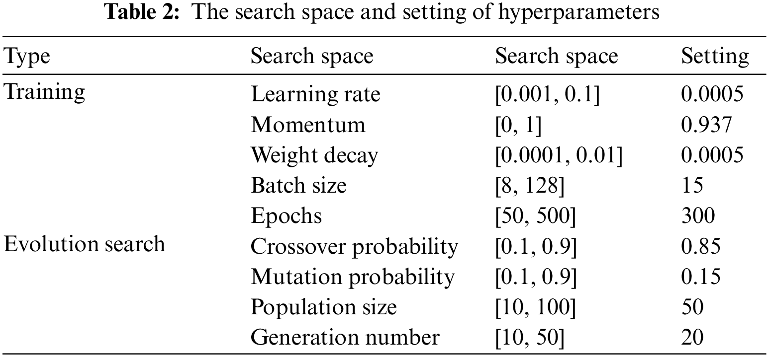
In this paper, the NAS method is used to optimize the hyperparameters, and the search space and setting of hyperparameters is shown in Table 2. In addition, the number of input and output channels of the architecture is set to 32, 64, 128, 256. The number of RBs in the RBU, DBs in the DBU, and MBs in the MBU are set to 3–10. The pooling types are max and average. After the above experimental preparation, this paper uses YOLOv5s, YOLOv8n, YOLOv8 + FasterNet, YOLOv8 + FasterNet + XioU, YOLOv6s and EV-YOLOv8 (ours) to train the above training set.

4.2 Evaluation Metrics

In this paper, the EV-YOLOv8 model can reduce the number of parameters that need to be calculated for training and reduce the complexity of the network on the basis of ensuring that the detection accuracy is not reduced or even improved. Therefore, this paper selects mAP50, Parameters and GFLOPS as evaluation indicators.

mAP50, a key metric in object detection tasks, evaluates a model’s accuracy and recall across categories. A higher mAP50 suggests better classification and detection capabilities, signifying at least 50% overlap in prediction boxes. To determine mAP50, accuracy and recall for each category are first calculated using Eqs. (8) and (9).

P=TPTP+FP(8)

R=TPTP+FN(9)

where, P denotes the model’s prediction accuracy; R is the recall, or the fraction of actual targets correctly predicted. TP, FP, and FN stand for true positives (detections with IoU > 0.5), false positives (IoU ≤ 0.5), and false negatives (missed targets), respectively. AP for each category is calculated using Eq. (10) based on P and R.

AP=1mΣimPi=∫P(R)dR(10)

where, m is the count of positive examples among n samples. Pi is the highest accuracy for the i-th positive example. The final mAP50 is derived using Eq. (11).

mAP50=1C∑jCAPj(11)

where, C is the dataset’s number of categories, and APj is the mean accuracy per category. Additionally, parameters in a deep learning model, comprising weights and biases, are adjusted during training to improve data fit. They indicate the model’s size and complexity—more parameters often imply a larger model. This affects training and inference, potentially increasing computational and storage demands and risking overfitting. GLOPs measures the model’s execution speed in billions of floating-point operations per second, reflecting its computational needs, hardware requirements, and network complexity.

4.3 Results and Analysis

4.3.1 Fault Detection Results and Analysis

According to the above evaluation indicators, the ablation experiment comparison results carried out in this paper are shown in Table 3.

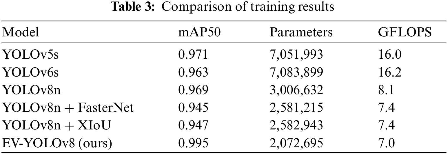
In Table 3, the mMap50 value of YOLOv5s for the above data set is slightly higher than that of YOLOv8n.This phenomenon is mainly due to the fact that the model size of YOLOv5s is larger than that of YOLOv8n. After adding the FasterNet module into the network architecture of YOLOv8n, the number of parameters and the complexity of the model are sharply reduced by 425,417 and 0.7, respectively, indicating that the purpose of lightweighting the model is achieved, but its mAP50 value is reduced by 1.2%. In order to increase the mAP50 value and further lighten the network model, this paper initially changes the loss function to XIoU_Loss. Although the improved mAP rise point is 0.2%, it is still 2.2% less than the mAP of YOLOv8n. In addition, the trained YOLOv6s model has a mAP50 value that is 0.8% lower than that of the YOLOv5s model. At the same time, the YOLOv6s model requires 31,906 more parameters to train compared to the YOLOv5s model. Through analysis, it is concluded that the decrease in detection accuracy of the YOLOv6s model is due to its insufficient capability in detecting small objects. The use of grid division detection method in the YOLOv6s model lacks robustness when the target scale changes, thus affecting the final detection accuracy. Furthermore, the YOLOv6s model has added many modules and technical details compared to the YOLOv5s model, resulting in a higher complexity of the network, requiring more computational parameters to train the YOLOv6s model.

In order to further improve the mAP value, and considering that the fault detection of the wind turbine blade surface is a small target detection, the loss function is changed to EfficiCIoU and the model is named EV-YOLOv8. The mAP value of the EV-YOLOv8 model is 2.6% higher than that of the YOLOv8n, the parameter amount is reduced by 933,937, and the GFLops is reduced by 0.9, which satisfies the purpose of reducing the number of parameters and reducing the amount of computation while increasing the mAP value.

4.3.2 Loss Function

The convergence of the loss function before and after improvement is shown in Fig. 4. A network model that incorporates the XIoU loss function for improvement is constructed [44]. By dividing the boundary distance by the intersection area as a penalty term, the quality of the box without overlap can be evaluated more effectively. In the Fig. 4, box_loss represents the box regression loss which is used to evaluate the position accuracy and precision of the prediction box. The goal of box_loss is to minimize the discrepancy between the predicted box and the actual box. cls_loss represents the classification loss, which is used to evaluate the classification accuracy of the model for the target object. dfl_loss represents the feature regression loss used for detecting and regressing the feature points of the target object.

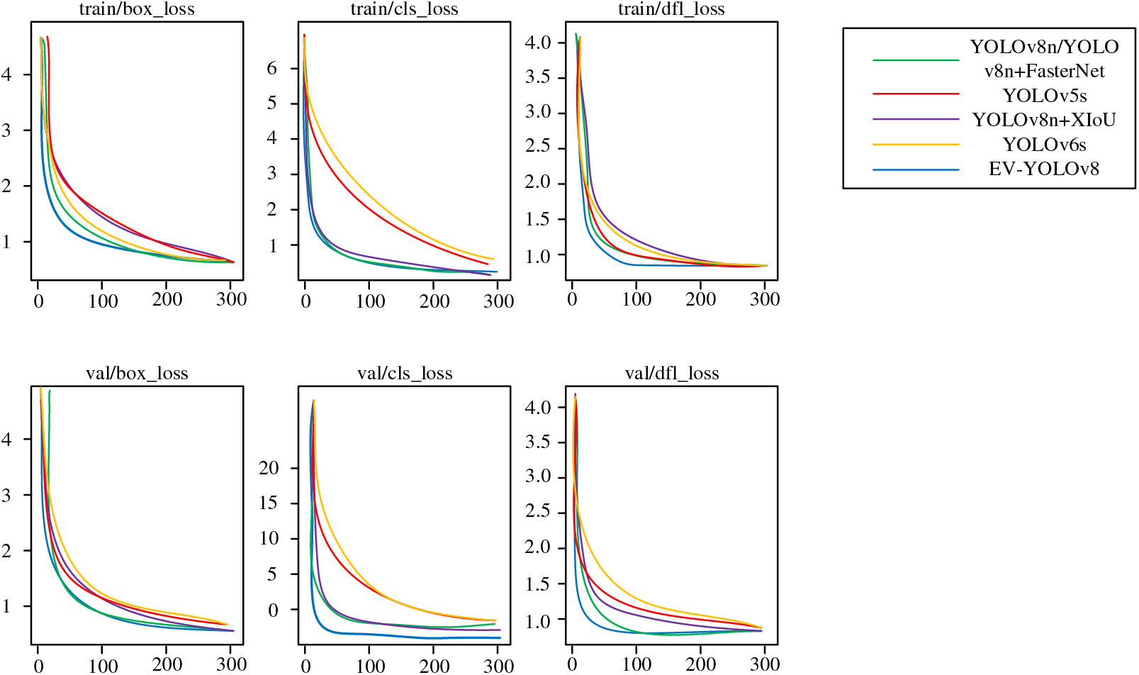
Figure 4: Loss function comparison chart

As shown in Fig. 4, the convergence speed of the three loss function curves of the EV-YOLOv8 model with the EfficientCIoU loss function is not only faster than the YOLOv8n and YOLOv5s models, but also faster than the YOLOv8 + XIoU model with the XIoU loss function. After the convergence of the three loss function curves, the box regression loss value of the EV-YOLOv8 model is also the lowest. After analysis, the reason for this phenomenon is that the center point distance term introduced by the EfficientCIoU loss function can describe the difference between the prediction box and the real box more comprehensively. In contrast, the XIoU loss function only considers the degree of overlap of bounding boxes, and may not be able to accurately evaluate some boxes with slight position offsets. Therefore, the EfficientCIoU loss function is more targeted and sensitive, and can guide the model convergence faster. In the Fig. 4, it can also be seen that the convergence of the loss function curve for the YOLOv6s model is not as good as that of other models. This is because the YOLOv6s model uses the SIoU concept to construct the loss function. The calculation method of the SIoU loss function is simpler compared to that of other loss functions. However, for extremely small targets or highly non-rectangular targets, the SIoU loss function may introduce significant errors. The SIoU loss function does not comprehensively consider factors such as scale, position, and shape in target detection tasks, thus lacking a certain level of comprehensiveness and robustness. Therefore, the SIoU loss function is not suitable for handling the complex multi-scale targets with varied backgrounds as used in this study.

Secondly, the introduction of the center point distance term makes the EfficientCIoU loss function measure the positional relationship of the target object more carefully. This helps the model to adjust the position of the prediction box faster and improve the accuracy of the detection. In contrast, the XIoU loss function only focuses on the overlap degree of the bounding box, which makes the XIoU loss function unable to guide the model to adjust the position well.

5  Conclusion

In the previous works, traditional fault detection methods limit network depth, hindering the discovery of optimal architectures for various tasks and resulting in oversized models difficult to deploy on devices with limited resources, such as smartwatches. Additionally, NAS, being resource-heavy, demands extensive GPU use, making the search for an ideal architecture expensive.

In this paper, we have proposed an evolutionary-based variational YOLOv8 design approach to address fault detection. Specifically, we first design an improvement of the FasterNet module based on the partial convolution operator. To enhance convergence performance, we improve the loss function based the efficient complete intersection over the union. Finally, a variable-length encoding approach is presented to represent network architectures of different depths. Experiment results confirm that the proposed approach can achieve excellent fault detection results. Future improvements to our method could address two main areas. First, reducing the need for manually setting numerous hyperparameters in the search space’s basic units to enhance fault detection task performance. We aim to widen the search space for more extensive hyperparameter coverage. Second, we plan to boost our method’s speed and effectiveness by combining population memory with information retrieval techniques, thereby refining our approach to efficiently navigate and optimize the neural architecture search space.

Acknowledgement: We thank all the members who have contributed to this work with us.

Funding Statement: This work was supported by the Liaoning Province Applied Basic Research Program Project of China (Grant: 2023JH2/101300065), and the Liaoning Province Science and Technology Plan Joint Fund (2023-MSLH-221).

Author Contributions: Conceptualization: Hongjiang Wang, Qingze Shen; Methodology: Qin Dai; Formal analysis: Yingcai Gao, Jing Gao; Writing-original draft preparation: Tian Zhang, Qingze Shen, Jing Gao; Writing review and editing: Hongjiang Wang, Tian Zhang. All authors reviewed the results and approved the final version of the manuscript.

Availability of Data and Materials: The data used to support the findings of this study are available from the corresponding author upon request.

Conflicts of Interest: The authors declare that they have no conflicts of interest to report regarding the present study.

References

1. Z. Liu, L. Zhang, and J. Carrasco, “Vibration analysis for large-scale wind turbine blade bearing fault detection with an empirical wavelet thresholding method,” Renew. Energy, vol. 146, no. 6, pp. 99–110, 2020. doi: 10.1016/j.renene.2019.06.094. [Google Scholar] [CrossRef]

2. G. Helbing and M. Ritter, “Deep Learning for fault detection in wind turbines,” Renew. Sustain. Energ. Rev., vol. 98, no. 3, pp. 189–198, 2018. doi: 10.1016/j.rser.2018.09.012. [Google Scholar] [CrossRef]

3. W. Nick, J. Shelton, K. Asamene, and A. C. Esterline, “A study of supervised machine learning techniques for structural health monitoring,” MAICS, vol. 1353, pp. 36, 2015. [Google Scholar]

4. L. Deng, Y. Guo, and B. Chai, “Defect detection on a wind turbine blade based on digital image processing,” Processes, vol. 9, no. 8, pp. 1452, 2021. doi: 10.3390/pr9081452. [Google Scholar] [CrossRef]

5. J. Wei and J. McCarty, “Acoustic emission evaluation of composite wind turbine blades during fatigue testing,” Wind Eng., vol. 17, no. 6, pp. 266–274, Jan. 01, 1993. [Google Scholar]

6. N. Li, L. Ma, G. Yu, B. Xue, M. Zhang and Y. Jin, “Survey on evolutionary deep learning: Principles, algorithms, applications, and open issues,” ACM Comput. Surv., vol. 56, no. 2, pp. 1–34, 2023. doi: 10.1145/3659100. [Google Scholar] [CrossRef]

7. A. Voulodimos, N. Doulamis, A. Doulamis, and E. Protopapadakis, “Deep learning for computer vision: A brief review,” Comput. Intell. Neurosci., vol. 2018, pp. 1–13, 2018. doi: 10.1155/2018/7068349. [Google Scholar] [PubMed] [CrossRef]

8. L. Zhao et al., “MESON: A mobility-aware dependent task offloading scheme for urban vehicular edge computing,” IEEE Trans. Mob. Comput., vol. 23, no. 5, pp. 4259–4272, May 2024. doi: 10.1109/TMC.2023.3289611. [Google Scholar] [CrossRef]

9. J. Redmon, S. Divvala, R. Girshick, and A. Farhadi, “You only look once: Unified, real-time object detection,” in Proc. IEEE Conf. Comput. Vis. Pattern Recognit., Las Vegas, LV, USA, 2016, pp. 779–788. [Google Scholar]

10. G. Jocher et al., “ultralytics/yolov5: v5.0–YOLOv5-P6 1280 models, AWS, Supervisely and YouTube integrations,” Zenodo, 2021. doi: 10.5281/zenodo.4679653. [Google Scholar] [CrossRef]

11. P. Ren et al., “A comprehensive survey of neural architecture search: Challenges and solutions,” ACM Comput. Surv., vol. 54, no. 4, pp. 1–34, 2021. [Google Scholar]

12. B. Zoph and Q. V. Le, “Neural architecture search with reinforcement learning,” arXiv preprint arXiv:1611.01578, 2016. [Google Scholar]

13. H. Liu, K. Simonyan, and Y. Yang, “Darts: Differentiable architecture search,” arXiv preprint arXiv:1806.09055, 2018. [Google Scholar]

14. Y. Liu, Y. Sun, B. Xue, M. Zhang, G. G. Yen and K. C. Tan, “A survey on evolutionary neural architecture search,” IEEE Trans. Neural Netw. Learn. Syst., vol. 34, no. 2, pp. 550–570, 2021. doi: 10.1109/TNNLS.2021.3100554. [Google Scholar] [PubMed] [CrossRef]

15. R. Girshick, J. Donahue, T. Darrell, and J. Malik, “Rich feature hierarchies for accurate object detection and semantic segmentation,” in Proc. IEEE Conf. Comput. Vis. Pattern Recognit., USA, 2014, pp. 580–587. [Google Scholar]

16. R. Girshick, “Fast r-cnn,” in Proc. IEEE Int. Conf. Comput. Vis., Washington, USA, 2015, pp. 1440–1448. [Google Scholar]

17. J. Guo, C. Liu, J. Cao, and D. Jiang, “Damage identification of wind turbine blades with deep convolutional neural networks,” Renew. Energy, vol. 174, no. 1, pp. 122–133, 2021. doi: 10.1016/j.renene.2021.04.040. [Google Scholar] [CrossRef]

18. X. Cheng, F. Shi, M. Zhao, G. Li, H. Zhang and S. Chen, “Temporal attention convolutional neural network for estimation of icing probability on wind turbine blades,” IEEE Trans. Ind. Electron., vol. 69, no. 6, pp. 6371–6380, 2021. doi: 10.1109/TIE.2021.3090702. [Google Scholar] [CrossRef]

19. J. Redmon and A. Farhadi, “YOLO9000: Better, faster, stronger,” in Proc. IEEE Conf. Comput. Vis. Pattern Recognit., Honolulu, HI, USA, 2017, pp. 7263–7271. [Google Scholar]

20. J. Redmon and A. Farhadi, “YOLOv3: An incremental improvement,” arXiv preprint arXiv:1804.02767, 2018. [Google Scholar]

21. A. Bochkovskiy, C. Y. Wang, and H. Y. M. Liao, “YOLOv4: Optimal speed and accuracy of object detection,” arXiv preprint arXiv:2004.10934, 2020. [Google Scholar]

22. C. Li et al., “YOLOv6: A single-stage object detection framework for industrial applications,” arXiv preprint arXiv:2209.02976, 2022. [Google Scholar]

23. C. Y. Wang, A. Bochkovskiy, and H. Y. M. Liao, “YOLOv7: Trainable bag-of-freebies sets new state-of-the-art for real-time object detectors,” in Proc. IEEE/CVF Conf. Comput. Vis. Pattern Recognit., Vancouver, BC, Canada, 2023, pp. 7464–7475. [Google Scholar]

24. H. Lou et al., “DC-YOLOv8: Small-size object detection algorithm based on camera sensor,” Electronics, vol. 12, no. 10, pp. 2323, 2023. doi: 10.3390/electronics12102323. [Google Scholar] [CrossRef]

25. Y. Yao, G. Wang, and J. Fan, “WT-YOLOX: An efficient detection algorithm for wind turbine blade damage based on YOLOX,” Energies, vol. 16, no. 9, pp. 3776, 2023. doi: 10.3390/en16093776. [Google Scholar] [CrossRef]

26. R. Zhang and C. Wen, “SOD-YOLO: A small target defect detection algorithm for wind turbine blades based on improved YOLOv5,” Advcd. Theory and Sims., vol. 5, no. 7, pp. 2100631, 2022. doi: 10.1002/adts.202100631. [Google Scholar] [CrossRef]

27. L. Ma et al., “Pareto-wise ranking classifier for multi-objective evolutionary neural architecture search,” IEEE Trans. Evol. Comput., p. 1, 2023. [Google Scholar]

28. L. Ma et al., “Learning to optimize: Reference vector reinforcement learning adaption to constrained many-objective optimization of industrial copper burdening system,” IEEE Trans. Cybern., vol. 52, no. 12, pp. 12698–12711, 2021. doi: 10.1109/TCYB.2021.3086501. [Google Scholar] [PubMed] [CrossRef]

29. Y. Xue, C. Chen, and A. Słowik, “Neural architecture search based on a multi-objective evolutionary algorithm with probability stack,” IEEE Trans. Evol. Comput., vol. 27, no. 4, pp. 778–786, 2023. doi: 10.1109/TEVC.2023.3252612. [Google Scholar] [CrossRef]

30. T. Zhang, C. Lei, Z. Zhang, X. B. Meng, and C. P. Chen, “AS-NAS: Adaptive scalable neural architecture search with reinforced evolutionary algorithm for deep learning,” IEEE Trans. Evol. Comput., vol. 25, no. 5, pp. 830–841, 2021. doi: 10.1109/TEVC.2021.3061466. [Google Scholar] [CrossRef]

31. B. Zoph, V. Vasudevan, J. Shlens, and Q. V. Le, “Learning transferable architectures for scalable image recognition,” in Proc. IEEE Conf. Comput. Vis. Pattern Recognit., Salt Lake City, UT, USA, 2018, pp. 8697–8710. [Google Scholar]

32. W. Wen, H. Liu, Y. Chen, H. Li, G. Bender and P. J. Kindermans, “Neural predictor for neural architecture search,” in Eur. Conf. Comput. Vis, Springer, 2020, pp. 660–676. [Google Scholar]

33. Y. Xu et al., “ReNAS: Relativistic evaluation of neural architecture search,” in Proc. IEEE/CVF Conf. Comput. Vis. Pattern Recognit., 2021, pp. 4411–4420. [Google Scholar]

34. L. Ma, H. Kang, G. Yu, Q. Li, and Q. He, “Single-domain generalized predictor for neural architecture search system,” IEEE Trans. Comput., vol. 73, no. 5, pp. 1400–1413, 2024. doi: 10.1109/TC.2024.3365949. [Google Scholar] [CrossRef]

35. T. Zhang, L. Ma, Q. Liu, N. Li, and Y. Liu, “Genetic programming for ensemble learning in face recognition,” in Int. Conf. Sensing and Imaging, Springer, 2022, pp. 209–218. [Google Scholar]

36. N. Nedjah, L. D. M. Mourelle, and R. G. Morais, “Inspiration-wise swarm intelligence meta-heuristics for continuous optimisation: A survey-part III,” Int. J. Bioinspired Comput., vol. 17, no. 4, pp. 199–214, 2021. doi: 10.1504/IJBIC.2021.116578. [Google Scholar] [CrossRef]

37. L. Ma et al., “A novel fuzzy neural network architecture search framework for defect recognition with uncertainties,” IEEE Trans. Fuzzy Syst., vol. 32, no. 5, pp. 3274–3285, May 2024. doi: 10.1109/TFUZZ.2024.3373792. [Google Scholar] [CrossRef]

38. L. Zhao et al., “Adaptive swarm intelligent offloading based on digital twin-assisted prediction in VEC,” IEEE Trans. Mob. Comput., pp. 1–18, 2023. doi: 10.1109/TMC.2023.3344645. [Google Scholar] [CrossRef]

39. M. Sessarego, K. Dixon, D. Rival, and D. Wood, “A hybrid multi-objective evolutionary algorithm for wind-turbine blade optimization,” Eng. Optim., vol. 47, no. 8, pp. 1043–1062, 2015. doi: 10.1080/0305215X.2014.941532. [Google Scholar] [CrossRef]

40. J. Bukala, K. Damaziak, H. R. Karimi, J. Malachowski, and K. G. Robbersmyr, “Evolutionary computing methodology for small wind turbine supporting structures,” Int. J. Adv. Manuf. Technol., vol. 100, no. 9-12, pp. 2741–2752, 2019. doi: 10.1007/s00170-018-2860-6. [Google Scholar] [CrossRef]

41. J. Chen et al., “Run, don’t walk: Chasing higher FLOPS for faster neural networks,” in Proc. IEEE/CVF Conf. Comput. Vis. Pattern Recognit., Hawaii, HI, USA, 2023, pp. 12021–12031. [Google Scholar]

42. Z. Zheng et al., “Enhancing geometric factors in model learning and inference for object detection and instance segmentation,” IEEE Trans. Cybern., vol. 52, no. 8, pp. 8574–8586, 2021. doi: 10.1109/TCYB.2021.3095305. [Google Scholar] [PubMed] [CrossRef]

43. Y. F. Zhang, W. Ren, Z. Zhang, Z. Jia, L. Wang and T. Tan, “Focal and efficient IOU loss for accurate bounding box regression,” Neurocomputing, vol. 506, no. 9, pp. 146–157, 2022. doi: 10.1016/j.neucom.2022.07.042. [Google Scholar] [CrossRef]

44. A. ElSaid, J. Karns, Z. Lyu, A. G. Ororbia, and T. Desell, “Continuous ant-based neural topology search,” in Int. Conf. Appl. Evol. Comput., Springer, 2021, pp. 291–306. [Google Scholar]