A New Speed Limit Recognition Methodology Based on Ensemble Learning: Hardware Validation

1  Introduction

Road transportation is considered as the most widely used mode of transport in the world. Unfortunately, this situation has led to an increased number of traffic accidents, which has numerous negative drawbacks for public health, the economy, and society. According to the World Health Organization (WHO), about 1.3 million people die and about 50 million get injured every year. Moreover, in 2016, a study carried out by the National Highway Transportation Safety Administration (NHTSA) revealed that 94% of vehicle accidents are caused either by driver negligence, misinterpretation of the road signs, or non-compliance with them. Therefore, it is imperative to deploy automated and/or intelligent systems either to aid the driver in decision-making or to potentially replace the driver and autonomously make appropriate decisions.

In recent years, research and development of intelligent driving have been the topic of several initiatives and studies since there have been considerable breakthroughs in the performance of onboard equipment in vehicles. These advancements have allowed automotive manufacturers to include the following systems: Advanced Driver Assistance Systems (ADAS) and Automated Driving Systems (ADS), both belonging to Driver Automation (DA) [1] and offering various levels of autonomy and safety for drivers. In fact, the study [2] underlines the importance of ADAS in enhancing the mobility of older drivers by assisting them on unfamiliar roads and mitigating age-related impairments that may affect driving abilities. In addition, the Auto Outlook 2040 report by Deepwater Asset Management predicts that by 2040, over 90% of all vehicles sold will fall into the categories of Level 4 and Level 5 automation [3]. According to the American auto insurers’ statistics, vehicles equipped with collision warning systems that alert the driver of an imminent danger or equipped with automatic braking systems cause fewer accidents compared to those without such features. For example, at Mercedes, the use of a forward collision warning system has resulted in a 3% reduction in accident frequency, according to a report published by the Insurance Institute for Highway Safety.

In the context of intelligent and/or autonomous vehicles and the enhancement of road safety, the suggested methodology involves acquiring and analyzing a real-time video stream from a camera mounted on the dashboard of a vehicle to recognize encountered signs. Such methodology serves a dual purpose: in the case of ADAS, it displays and informs the driver about the nature of the sign, and in the case of ADS, it enables the appropriate decision-making for driving and vehicle control. One of the most impacting challenges of a Traffic Sign Recognition (TSR) system is the rapidity and effectiveness of traffic sign recognition in real-world scenes, especially when the vehicle is moving at high speed in critical weather conditions. Indeed, several parameters influence the detection and classification of signs, such as fog, rain, sandstorms, snow, differences in brightness between day and night, similar objects, degradation of sign quality, partial obstruction, etc. [4].

This paper focuses on the recognition speed limit signs, a special category of traffic signs from the German Traffic Sign Recognition Benchmark (GTSRB) dataset, that thanks to their pivotal role in guiding drivers have enhanced traffic safety therefore reducing the risk of accidents on the roads. For these reasons, the suggested real time Speed Limit Recognition (SLR) methodology includes three modules: a Speed Limit Detection (SLD) module aiming to detect the traffic sign in the captured frame using the Haar Cascade technique, a Speed Limit Classification (SLC) module in which Machine Learning (ML) classifiers (KNN, SVM and Random Forest) and a new developed deep learning model based on CNN called DeepSL focused on speed limit images from the GTSRB dataset. Due to various conditions of image capturing, road sign recognition is subject to uncertainties. As a result, a Speed Limit Classifiers Fusion (SLCF) module has been introduced in the suggested approach. This module combines trained ML classifiers and the DeepSL trained model by using Data fusion techniques like Dempster Shafer’s (DS) theory of belief functions and voting classifier from Ensemble Learning. These methods are employed to identify the most accurate combination of classifiers to improve the recognition process. In order to validate the effectiveness and the reliability of the proposed SLR methodology, a prototype including all software and hardware components is developed and tested initially, by simulation using video sequences and secondly, by using electronic targets such as Raspberry Pi 4 Model B and Nvidea Nano Jetson.

Remaining sections have been organized as follows: Section 2 describes different road signs found in the driving environment and summarizes methods used to detect and classify them. Section 3 details the suggested SLR methodology and discusses the obtained results. Section 4 illustrates the developed prototype of the elaborated SLR system. Finally, the last section is dedicated to a conclusion and the suggestion of potential future work.

2  Related Works

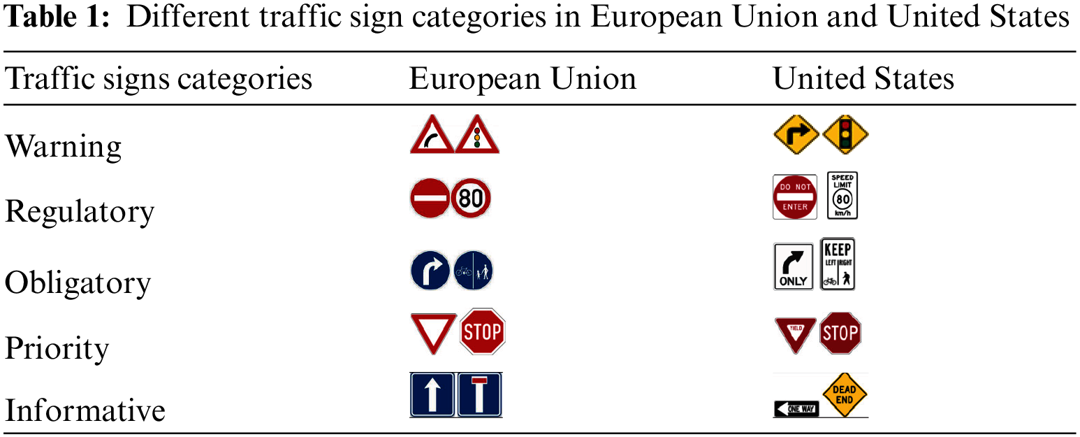
In the driving environment, various kinds of traffic signs have been installed to ensure safety on roads. Every road sign has a certain purpose, such as indicating which way to go, informing drivers about the rules of road, notifying of a danger, crossing, etc. In addition, some road signs have the same meaning around the world but look different. Table 1 shows an example of the different categories of signs used on European and American roads [5].

In recent research, TSR systems have been widely studied. It has been understood that they are developed by using road sign detection and classification methods on various traffic signs datasets like GTSRB [6], DITS (Dataset of Italian Traffic Signs) [7], BTSD (Belgium Traffic Sign Dataset) [8], RTSD (Russian Traffic Sign Dataset) [9]. In fact, a TSR system aims to recognize a road sign from an image and instantly transmits the result to the driver, either through a display on the dashboard or an audible signal in the case of ADAS, or a command signal that interacts with the vehicle’s driving equipment (braking, steering, acceleration, etc.) in the case of ADS. However, the TSR’s ability to accurately identify a sign depends on the vehicle’s speed and the distance between the vehicle and the sign. One notable work by [10] introduced a deep learning-based approach, specifically YOLOv5, which achieved high accuracy of up to 97.70% and a faster recognition speed of 30 fps compared to SSD. Additionally, a study in [11] emphasized the use of finely crafted features and dimension reduction techniques to enhance traffic sign recognition accuracy to 93.98%. These works highlight the advantages of improved accuracy and faster recognition speeds in TSR systems. However, challenges such as environmental restrictions, limited driving conditions, and the need for continuous dataset expansion remain as notable disadvantages in the field [10,11].

The process of recognition relies on five stages: image capture, preprocessing, detection, classification, and decision-making, as shown in Fig. 1.

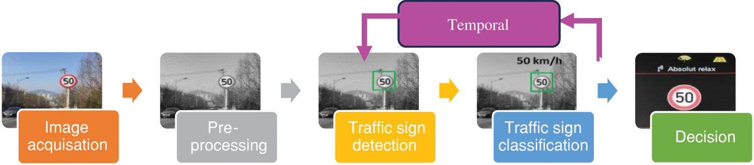
Figure 1: General architecture of TSR system

Initially, the image acquired from onboard camera(s) in a vehicle is cleaned and prepared through processes such as correcting image distortion, changing dimensions, and eliminating noise are carried out. These activities aim to make the image more suitable for in-depth analysis in subsequent stages. The system then utilizes object detection algorithms to locate road signs in the pre-processed images, which are subsequently classified according to their meanings. Finally, the system uses the obtained information to alert the driver to decision-making or to transmit commands to other vehicle components. In most TSR systems, the detection step is dissociated and independent from the classification step. This dissociation can lead to certain malfunctions such as false detections, multiple detection for the same panel, failure of detection due to temporary occultations, etc. In order to overcome these problems, it is possible to add a time tracking step for the processing of video sequences [12] as illustrated in Fig. 1. Indeed, this process makes it possible to consider the redundancy of a traffic sign in several consecutive frames before its disappearance from the camera’s field of vision in order to confirm its presence [13].

2.1 Image Acquisition

The onboard camera of the TSR system ensures the real-time acquisition of images related to the driving environment. The quality of the captured images can impact the reliability and accuracy of the detected sign information. Hence, it is crucial to equip the system with a high-quality camera to guarantee optimal performance.

2.2 Pre-Processing

A road sign is typically exposed to various challenges in its environment, such as varying brightness, diverse weather conditions, viewing angle issues, damage, or partial obstruction which in turn can lead to variable visibility or various traffic sign appearances, a chaotic background, and poor image quality caused by high speeds. To mitigate the impact of these challenges, serval preprocessing techniques are employed at the initial stage to eliminate noise, reduce complexity, and enhance overall sensitivity and recognition accuracy. The most used preprocessing techniques include normalization, noise removal, and image binarization. These techniques can be applied individually or in a combination to improve image quality and facilitate sign detection. A pre-processed image then undergoes the next step, which is the detection process.

2.3 Traffic Sign Detection (TSD) Methods

The aim of the traffic sign detection is to identify traffic sign sizes and locations in real visual scenarios. The speed and efficiency of the detection process are crucial elements that significantly impact the overall system. Their role is to minimize the search area and only pinpoint the road sign present in the captured image. Many approaches for detecting traffic signs depend on attributes such as the sign’s color and shape, or leverage machine and deep learning methods.

Color-based traffic sign detection methods seek to identify the region of interest (ROI) in a captured image based on the colors of traffic sign. According to [14], they are remarkably affected by illumination, the daytime, weather conditions, color and surface reflection of the sign. Shape-based traffic sign detection methods entail the process of identifying and estimating contours, which then lead to a decision based on the count of these contours [15]. Experiments show that these approaches are more reliable than colorimetric techniques because they are not affected by variations in daylight or colors. Yet, they are sensitive to small and ambiguous signs, need a large capacity of memory and time-consuming calculations [16]. Color and shape-based detection methods are a combination of color and shape characteristics [17]. Typically, they depend on appropriate parameters and effective color enhancement results [14,15]. Various factors, including changes in lighting, occlusions, translations, rotation, and scale change, are lacking, however.

Methods based on ML and deep learning can detect traffic signs accurately and address the short comings of the previous methods, such as lighting changes, occlusions, translations, rotation, and scale change. Most ML based detection methods, such as AdaBoost detection technique and SVM algorithm, employ handcrafted features for extracting the traffic sign whereas deep learning-based detection methods learn features through CNN (Convolutional Neural Network). In fact, the Haar-like Cascade technique has been developed by [18]. It involves a cascade of Haar-like features to identify objects within images. Support Vector Machine (SVM) employs HOG-like features to characterize and detect objects as an SVM classification problem. In this situation, each potential area of interest is categorized as either containing objects or being part of the background [19]. According to [20], using Haar-like Cascade features is faster and more useful in detecting faded and blurry traffic signs in different lighting conditions than HOG-like features.

In general, CNN-based detection networks which are deep learning techniques, tends to be slow. Nonetheless, there are networks like You Only Look Once (YOLO) that demonstrate swift and efficient performance. Yet, some networks, such as You Only Look Once (YOLO), have fast performance [21]. Using the German Traffic Sign Detection Benchmark dataset (GTSDB) and Faster RCNN 84.5% in 261 ms are achieved, compared to 94.2% in 155 ms using the standard RCNN algorithm for Haar like cascade technique [22]. Furthermore, ROI extraction is not necessary for AdaBoost-based approaches, unlike SVM-based approaches, which have a substantial effect on the efficiency of SVM-based TSD detectors.

2.4 Traffic Sign Classification (TSC) Methods

The TSC step is the third stage in the TSR process. It concerns standard computer vision and ML techniques. These methods are replaced later by deep learning models. In fact, ML based classification methods involve two major phases: First, image features are extracted to emphasize distinction between classes. Subsequently, they undergo classification through ML algorithms. Hand-crafted features including Histogram of Oriented Gradients (HOG) which focuses on the structure or shape of an object [23], Locally Binary Patterns (LBP) describes the texture of an image [24] and Gabor filter is used for edge detection, texture recognition, and image segmentation [19]. These manually designed features are frequently employed in conjunction with ML classifiers like KNN (K-Nearest Neighbors), Random Forest, and SVM (Support Vector Machine) [25].

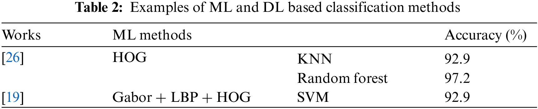
Table 2 displays examples derived from the application of ML based classification methods on the GTSRB dataset. As detailed in [26], HOG features are utilized with KNN and Random Forest classifiers, yielding accuracy percentages of 92.9% and 97.2%, respectively. Additionally, another study referenced by [19] employs a combination of Gabor, LBP and HOG features in conjunction with a SVM classifier, achieving an accuracy rate of 92.9%.

According to DL classification methods, they are based on ConvNets (CNNs). In fact, a CNN extracts features from images through the training of a multitude of hidden layers on a set of images. Hence, the deeper the network is, the more exclusive and informative the features become, with reduced redundancy. In [27], authors suggest using 3CNNs, a new variant of their previous model (CNN) and they achieve 99.70% compared to 99.51% on GTSRB. Additionally, another study referenced by [28] propose a TSC method using CNNs, which achieved an accuracy level of 99.6% on the validation set on the GTSRB dataset. Based on these results, DL methods based on CNN demonstrate superior accuracy and robustness in classifying traffic signs. These findings highlight the potential of DL approaches to enhance road safety and traffic management systems.

2.5 Decision

The decision-making step in the TSR system involves finding the type of existing sign in the image and determining the appropriate action based on its type such as displaying a warning signal on the dashboard, sounding an audible alert indicating the nature of the sign, or even transmitting a command signal to other vehicle equipment. It is crucial for the TSR system to be capable of making quick and accurate decisions, as an error in sign detection can lead to dangerous consequences for road users. For this very reason, these systems require rigorous testing and continuous improvement to ensure their effectiveness and adaptability to changes in the environment.

2.6 Temporal Tracking

Temporal tracking identifies previously recognized signs to avoid reclassifying them, which reduces processing time. The step of grouping the data, linking known signs (previously recognized) with perceived signs (detected at the current moment), ensures this identification. This coupling helps prevent signaling the same signs to the driver again, avoiding unnecessary disturbances.

A study by [29] highlights different problems of existing TSR systems that have reduced their robustness when tested in various illumination scenarios, leading to a significant drop in performance in low or strong lighting conditions. Additionally, these systems struggle with scalability, primarily due to a lack of diverse and high-quality training data. Lack of transparency in decision-making is also a common issue with TSR systems, making debugging and gaining trust challenging. Furthermore, existing TSR systems have difficulty accurately recognizing rare or new road signs that are not present during their training period, posing a potential road hazard in real-world situations, especially during cross-country travel where traffic signs can differ significantly. To address these constraints, the following section describes a new SLR methodology, aiming to fulfill the real-time, robustness, and accuracy requirements.

3  Proposed SLR Methodology

The accuracy and the fast-processing time are extremely important for a robust and efficient SLR system. Thus, the proposed SLR methodology satisfies these two constraints. Moreover, it is based on three modules: Speed Limit Detection (SLD), Traffic Sign Classification (SLC) and Traffic Sign Classifiers Fusion (SLCF). Different steps of the SLR system are summarized in the algorithm below:

Step 1:   Prepare the speed limit Haar cascade detector.

Step 2:   a) Develop a deep neural network for speed limit signs (DeepSL).

b) Train and test KNN, SVM, RF and DeepSL on speed limit images of the GTSRB dataset.

c) Save trained KNN, SVM, RF and DeepSL.

Step 3:   Fuse classifiers using a data fusion technique.

Step 4:   Capture frame from the video camera.

Step 5:   Extract the ROI from the frame by using the Haar cascade detector.

Step 6:   Predict detected ROI by using the most accurate combination.

Fig. 2 illustrates how the SL sign recognition process starts with a real-time camera frame capture. Then, a list of pre-processing treatments drawn up for each captured frame like resizing the image and applying filters on the image. A pre-processed image is after that treated by the SLD module which uses a speed limit Haar cascade detector to extract the ROI (SL sign). In the SLC module, SVM, KNN, RF and the newly developed ConvNet model (DeepSL) are trained on SL images from the GTSRB dataset and then saved onto the local disk to be used later in the Speed Limit Classifiers Fusion (SLCF). As a matter of fact, different combinations of classifiers are established after using fusion techniques like Dempster Shafer theory and the voting technique from EL. The output of the SLCF module is the most accurate combination of classifiers used to predict the detected SL sign.

Figure 2: Proposed speed limit recognition methodology

3.1 Speed Limit Detection (SLD) Module

The rate and the time processing for the detection of road signs are important factors to minimize the area of detection and indicate only potential regions. Hence, the Haar Cascade method is used to extract Regions of Interest (ROIs) from the captured frame. The Haar-like Cascade method is an object detection algorithm used to identify faces in a real-time image or video [18] and then used for detecting other objects. Indeed, this detector extracts first the Haar-like features from an input image and builds cascaded classifiers which are embedded into one strong detector (Adaboost: Adaptive boosting) able to discard negative images quickly and identify the candidate region of traffic sign.

3.2 Speed Limit Classification (SLC) Module

The performance of an automatic SLR system must firstly be validated first using a publicly accessible dataset. Therefore, speed limit images from the GTSRB dataset are used to train and evaluate ML classifiers (SVM, KNN, and Random Forest) and the developed deep learning model with CNN called DeepSL.

3.2.1 Speed Limit Dataset

The GTSRB is a large, organized, and open-source dataset used for developing classification machine learning models for traffic sign recognition. It contains more than 50,000 images, with over 39,000 images in the training set and 12,630 images in the test set, classified into more than 40 classes [30]. The dataset is widely used for traffic sign recognition tasks and has been used in numerous studies to evaluate the performance of various machine learning algorithms. In this work, nine speed limit classes (20, 30, 50, 70, 80, end of 80, 100 and 120 km/h) from the GTSRB dataset are used with approximately 13,200 images taken under different conditions (blurring, lighting, etc.) and presents noises like pixelization, low resolution, and low contrast of traffic sign images. In addition, the distribution of samples for each class is unbalanced. Actually, the largest classes (major) contain 10 times as many images of traffic signs as the smallest classes (minor) as in reality some signs, such as 50 km/h, appear more frequently than others.

3.2.2 Classification Metrics

In order to evaluate the classification process, various metrics are used:

Accuracy=True positives+True negatifsTrue positives+False positives+True negatifs+False negatifs (1)

Precision=True positivesTrue positives+False positives(2)

Recall=True positivesTrue positives+False negatives(3)

F1=2∗Precision∗RecallPrecision+Recall(4)

In this work, speed limit classes have unbalanced distributions. For this, the weighted-averaged (precision, recall, F1) score is used to increase the lowest scores. Google Collaboratory is used as a framework for training and testing SVM, KNN, Random Forest and (DeepSL) on speed limit classes from the GTSRB dataset.

3.2.3 Speed Limit Classification Results Using ML Classifiers

Machine learning classifiers such as KNN, SVM, and Random Forest are used for traffic sign classification due to their specific advantages. In fact, KNN is simple, adaptable, and suitable for multi-class problems, while SVM excels in high-dimensional spaces and can handle non-linearly separable data [31]. According to the Random Forest classifier, it requires less feature engineering and provides feature importance insights. These classifiers are used in various traffic sign recognition systems, such as the one described in [32] which uses KNN and SVM classifiers for their ability to provide good accuracy rates in road safety applications and the system in [33] that employs Random Forest for its ability to detect traffic signs under various conditions. As a result, these classifiers are used in order to train speed limit images using three feature descriptors: RGB colour descriptor, 3D colour histogram and HOG descriptor. Table 3 summarizes obtained F1 scores.

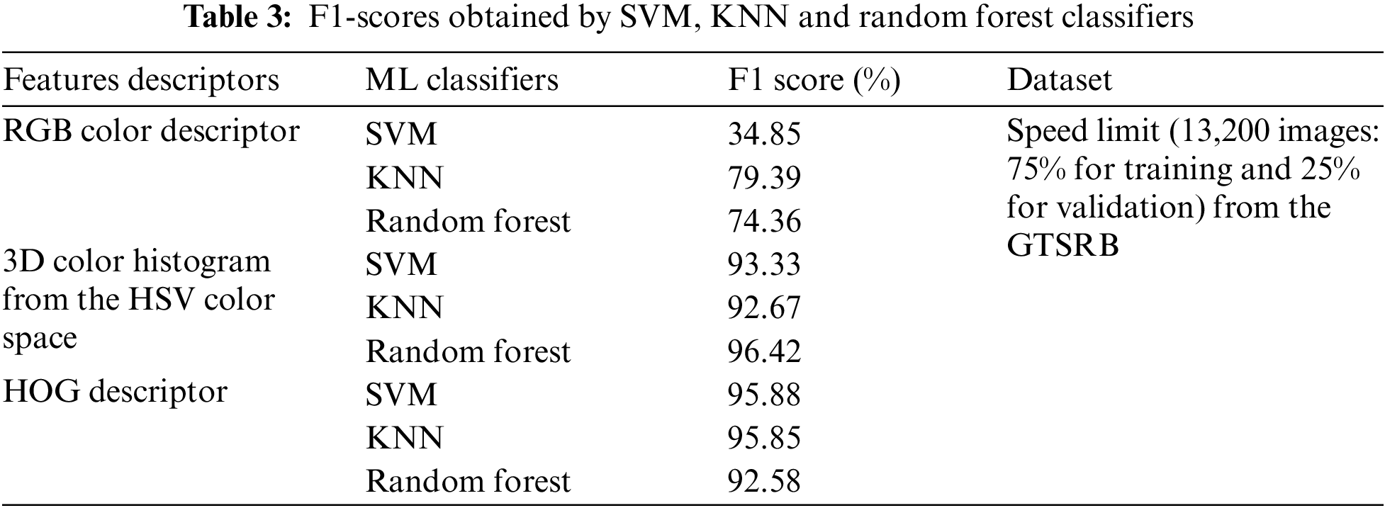
Table 4 explains reached F1 scores for each type of speed limit by applying ML classifiers (SVM, KNN and Random Forest) using the RGB colour feature descriptor (DF1), the 3D colour histogram descriptor (DF2) and the HOG descriptor (DF3). Results confirm that the SVM, KNN and RF classifiers used with the (DF2) ensure higher classification rates compared to the other results obtained with (DF1) and with (DF3).

3.2.4 Speed Limit Classification Results Using DeepSL Model

Recently and with the development of deep learning, diverse deep neural network architectures have appeared and have drawn a lot of academic and industrial interest [34]. In this context, DeepSL (Deep Speed Limit), a new ConvNet, for the classification of speed limit signs is developed and presents the architecture detailed as follows: the images (ROIs), in gray level, are transferred to a first convolutional layer (Conv2D) with 32 size filters (3 × 3), followed by a ReLU activation function to improve nonlinearity and model performance. This layer extracts features from grayscale images, such as edges and textures. A Batch Normalization layer follows the first convolutional layer. Next, a second Conv2D layer with the same settings as the first convolutional layer is added, followed by another Batch Normalization layer. This sequence of convolutional and normalization layers is repeated with filters of size 64. Between each pair of convolutional layers, a 2D Maxpooling layer of 2 × 2 size is added to extract the most important features. Dropout layers with a dropout rate of 0.25 are added after each Maxpooling layer to avoid overfitting. Once all the features have been extracted, a Flatten layer is used Then, a Dense layer of 512 neurons with a ReLU is added. A layer of Batch Normalization and another layer of Dropout with a deactivation rate of 0.5 are added. Lastly, a final last Dense layer of 9 neurons with a Softmax activation function is added to perform the classification of the input images into the 9 specified speed limit classes.

Table 5 shows experimental results found after training the model with 10 epochs on speed limit signs of the GTSRB dataset. We notice good F1 scores of classification results (>91%) in recognizing limit road signs.

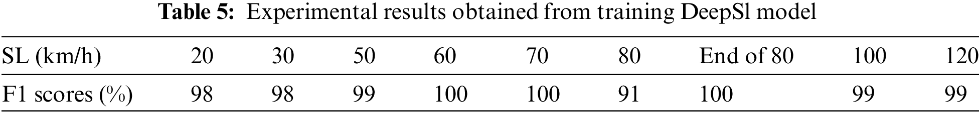
Table 6 shows that DeepSL model give a better classification rate of speed limit signs (98.8%) compared to those obtained by SVM, KNN and RF.

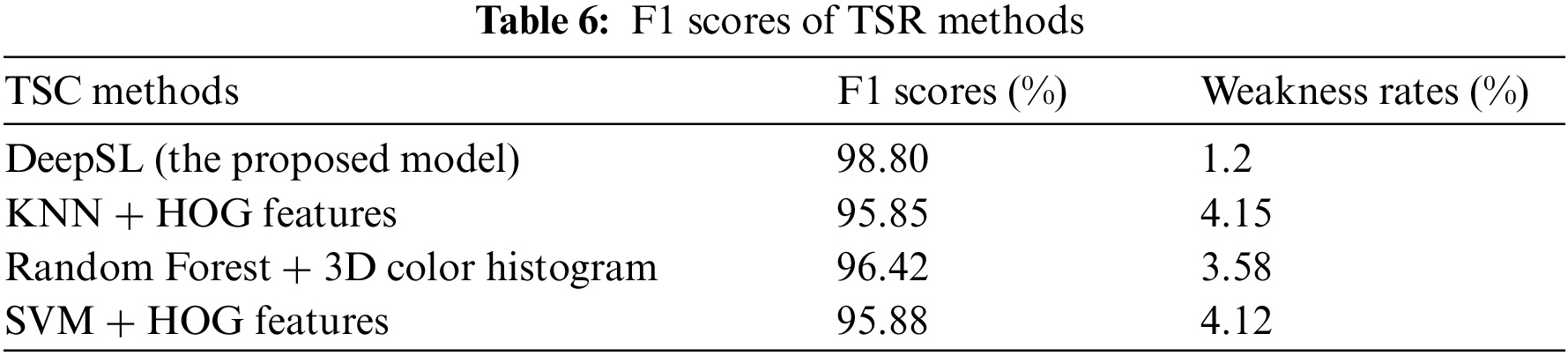
Table 7 summarizes best classification rates for each speed limit road sign obtained from applying Random Forest and DeepSL classifiers.

3.3 Speed Limit Classification Fusion (SLCF) Module

In the previous section, ML algorithms and the DeepSL model are used to classify different speed limit road signs with proportional accuracy rates. In fact, Table 6 shows the different weakness rate of each classifier that are respectively 1.2%, 4.15%, 3.58% and 4.12% for DeepSL, KNN, RF and SVM. Despite obtained good results, SLR system must have the minimum of possible errors to ensure road safety requirements and not be in a situation of uncertainty. In order to achieve lower classification error probability, classification rates can be improved by combining the results of classifiers to get benefit from the strengths of one method to overcome the weakness of another by using data fusion methods. Three non-exclusive categories can be used to group the available data fusion techniques: decision fusion, state estimation, and data association [35]. The decision fusion approach and the variety of classifier types have a major impact on a classification system’s performance. Accordingly, a classifiers fusion module is introduced in the proposed approach in order to fuse the various classifiers outputs in order to boost the final classification results and reduce decision conflicts.

First, relevant features are extracted from the input data using techniques such as traditional feature extraction or the use of convolutional neural networks (CNNs). Then, each classifier is trained on a separate training dataset by learning from the already extracted features and builds its own classification model. Once trained, each classifier is used individually to predict validation and test data. The predictions are then merged to a final decision. Finally, an evaluation of the fusion performance is carried out using metrics to enhance the fusion of the trained classifiers. The effectiveness of the decision fusion theory has been discussed in [36,37]. The most used strategies are the voting method, Bayesian theory, and the Dempster–Shafer evidence theory [38–41].

3.3.1 Dempster Shafer (DS) Theory

DS theory is a mathematical theory for reasoning under uncertainty, particularly in situations where there may be incomplete or conflicting evidence. It is presented first within the framework of statistical inference, and further expanded as an evidence theory [42]. Both supervised and unsupervised classification have used it. Unlike the Bayesian technique, the DS method explicitly accounts for unknown alternative sources of observed data. The DS technique uses probability and uncertainty intervals to assess the probability of hypotheses based on many pieces of data. Furthermore, it computes a probability for any valid hypothesis. When all the hypotheses investigated are mutually exclusive and the list of hypotheses is exhaustive, these two methods (DS and Bayesian theories) yield the same answers. In [43–46], Classifier outputs are represented as belief functions, which are then coupled with Dempster’s rule in the event of classifier fusion. In [37,47], the employed method involved converting the decisions made by the Support Vector Machine (SVM) classifiers into belief functions. In this work, DS theory has been chosen to be used rather than the other approaches since it permits the depiction of both imprecision and uncertainty data. The basics of DS theory are:

Mass function m defined by (5).

m:2Ω→[0,1]with∑A⊆Ωm(A)=1(5)

Correction of the information: The new mass function of the weakness operation is defined by (6).

m(A)=μ∗m(A);∀A≠Ω(6)

(m1⊕m2)(C)=∑A,B:C=A∩Bm1(A)∗m2(B)(7)

Information fusion: The new mass function after the use of Dempster’ rule is defined by (7).

Pignistic transformation (Decision making) defined by (8).

Betp(ω)=∑{A⊆Ω,ω∈A}m(A)(1−m(∅))|A|(8)

The decision will be made by choosing the element x with the greatest probability from pignistic transformation by applying (9).

Rp(x)=argmaxx∈ΩBetp(ω)(x)(9)

In this paper, DS theory is used by fusing two, three and four classifiers. 11 different forms of combinations (data fusion) between classifiers are possible based on the mass’s combination DS rule, given the mass function for each classifier (m1, m2, m3, and m4) of the DS theory, which correspond to the SVM, RF, KNN, and DeepSL classifiers. the decision on the outcomes following fusion is aided by the pignistic transformation of the acquired masses. Consequently, two, three and four classifiers are combined. Obtained results are 99.38% by fusing RF and DeepSL classifiers, 99.93% by fusing KNN, RF and DeepSL and 99.98% by fusing SVM, KNN, RF and DeepSL. Achieved results of classifiers combinations are shown in Table 8.

3.3.2 Ensemble Learning Methods

Ensemble Learning (EL) is a ML technique that involves combining multiple classifiers using various methods to produce a more accurate and reliable final decision, aiming to reduce classification errors and minimize the effects of information uncertainty. The different classifiers can be trained on distinct subsets of data or use different learning methods. The most common techniques in EL include bagging, boosting, stacking, and voting [48]. Bagging (Bootstrap Aggregation) creates multiple copies of the same model by training each copy in parallel on a random subset of the dataset using sampling techniques. Boosting involves sequentially training multiple relatively weak models, starting with an underfitting situation, and having each model correct the errors of its predecessor to form a complete and highly reliable final model. Two types of boosting exist: AdaBoost and Gradient Boosting. When two or more base models, or level 0 models, are used in a stacking (blending) process, a meta-model called the level 1 model is created by combining the predictions of the base models. Both hard and soft votes are supported by the voting technique. The class with the most votes, or the class having the highest likelihood of being predicted by each classifier, is the projected output class in a hard voting process. The forecast made for a class based on its average probability is known as the output class in soft voting.

In order to combine the proposed DeepSL model with the three ML classifiers (KNN, Random Forest and SVM), a fusion approach exploiting the characteristics of the input images is applied. Training and test image features are extracted from the pre-trained DeepSL model to capture complex patterns, textures, and relevant structures, resulting in high-quality features for each input image. These extracted features are then used separately to train each classifier independently. The voting method is chosen to merge classifiers. Table 9 summarizes the weighted rates of F1 as well as the weakness rates of KNN, RF, and SVM using DeepSL as the feature extractor. By combining the features extracted by DeepSL with the KNN, RF and SVM classifiers, one can exploit the advantages of both approaches (ML and DL) and improve the performance of image classification.

According to Table 10, it is remarkable that merging the ML classifiers using DeepSL as feature extractor improved the F1 score of the validation significantly compared to using each classifier separately. The combination of RF and KNN achieves the best F1 rate of 99.96%.

To validate the effectiveness and to confirm the performances of the proposed SLR solution, it is crucial to undergo two validation stages: software and practical validation.

4  Prototype of SLR System

4.1 Software Validation

Software validation is an essential step in ensuring that a system works effectively and reliably. There are two types of software validation: simulator validation, which uses interactive virtual environments similar to real life [49], and simulation validation, which tests road scenes full of road signs on a PC. In fact, enhancing systems through simulation-based validation using driving sequences on urban roads or freeways is a widely used method for testing and validating recognition systems, especially those related to traffic signs. In fact, this type of validation simulates different environmental driving conditions and evaluate the performance of the recognition system in a variety of scenarios. Hence, to validate the SLR system by simulation, two video sequences describing two road scenes rich in speed limit signs are used. The simulation is carried out by using a PC (configuration: Intel® Core (TM) i57200 CPU, 64-bit, 8 GB RAM) and Google Colab with 12.4 GB RAM. To evaluate the performance of the SLR system, processing time and the classification rate are calculated. Recognition time is calculated from the detection of the speed limit sign to its classification. The SLR system achieves an average of 0.06 s to identify each detected road sign in the case of computer simulation, and an average of 0.025 s using Google Colab. Fig. 3 shows examples of speed limit sign images recognized correctly by the SLR system in addition to their prediction rate using Google Colab.

Figure 3: Examples of speed limit signs correctly recognized by the SLR system

All speed limit signs located in the video sequence are well localized by the Haar Cascade detector and subsequently well recognized by applying the new model obtained from the vote fusion. However, two detected road signs are not correctly recognized by the SLR system, as shown in Fig. 4.

Figure 4: Examples of signs incorrectly recognized by the SLR system

In fact, the 40 km/h sign is detected as a speed limit sign, but misidentified because it is not included in the GTSRB learning base and the No passing sign is wrongly recognized once as a speed limit sign out of the three times it appeared.

4.2 Practical Validation

A system’s hardware architecture can vary according to its specific processing and performance requirements. Indeed, there are different hardware architectures based on CPU (Central Processing Unit), GPU (Graphic Processing Unit), FPGA (Field Programmable Gate Array) or heterogeneous by combining different types of units to take advantage of their specific benefits. For example, SoCs (System on Chip) combine two units in the same circuit to meet the criteria of an embedded system, i.e., dimensions, power consumption (autonomy), heat dissipation and speed of exchange between the two units.

In order to validate an architecture on a hardware target, several factors need to be considered, such as the performance of the core used for image processing (execution time and accuracy), the available memory and its type for efficient use of resources, and the availability of libraries and development tools to facilitate implementation, testing and subsequent improvements to the architecture. Based on the characteristics of the different board types already presented, the validation and evaluation of the SLR system will be carried out on Raspberry Pi 4 and Nano Jetson boards. Indeed, this choice is based on the specific technical characteristics of these two boards, summarized in Table 11, and their adaptability for artificial intelligence applications.

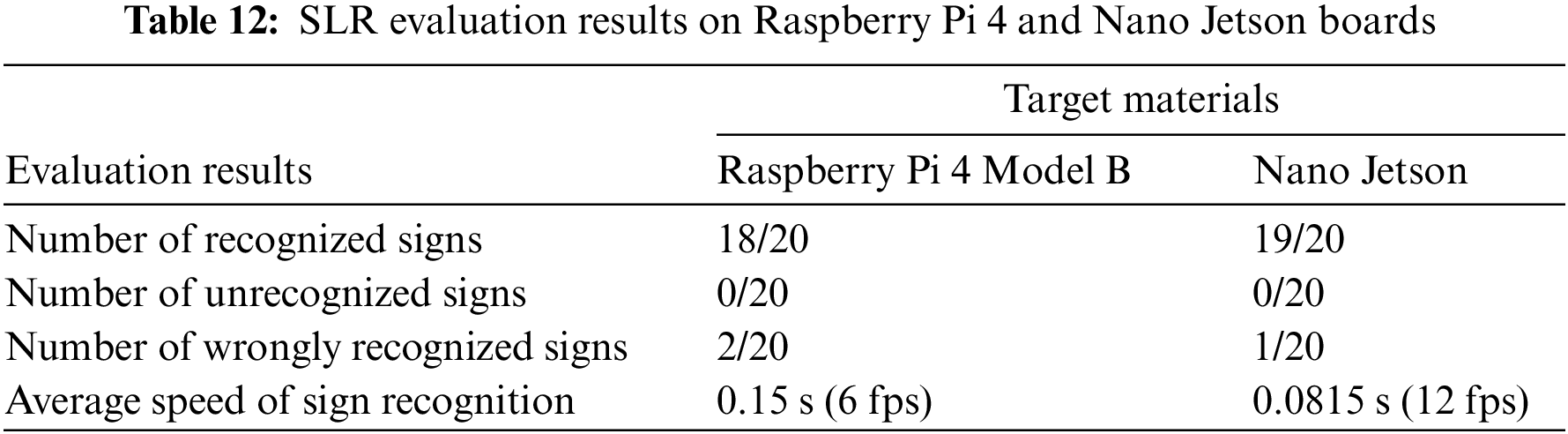
In order to ensure hardware validation, Raspberry Pi 4 and Jetson Nano boards are first configured with the needed software. Indeed, several useful libraries are installed, such as OpenCV, TensorFlow, Keras, as well as others required for the system to function properly. Then, the same driving sequences used previously for software validation are reused to achieve a hardware validation close as much as possible to the real driving environment. In this step, the on-board camera is positioned in front of the PC screen to capture the video sequences. Tests are carried out to evaluate the SLR system performance, such as processing speed and sign recognition rate. The processing speed represents the time required to detect and classify road signs, while the sign recognition rate represents the system’s accuracy in correctly recognizing road signs, by giving the number of correctly or incorrectly recognized or unrecognized signs in relation to the total number of signs. Obtained results are summarized in Table 12, which shows the performance of the SLR system on the two hardware platforms.

On the Raspberry Pi board, some experiments with the SLR system have been conducted. The authors’ first work in [50] is the development of a Raspberry Pi-based recognition system for speed limit signs, with consideration given to the stability of color detection with respect to daylight. According to the results, their system can process data in as little as two seconds and has an accuracy of 80%. In addition, a second study uses a Raspberry Pi 3 board and ML techniques to create a real-time sign recognition system that recognizes five different classes of signs, identifies their type, and notifies the driver. According to the results, the system’s maximum average time to identify the type of sign when the vehicle is moving at 50 km/h is 3.44 s, and the average accuracy of sign recognition for the five classes is over 90% [51].

Considering Table 12, the proposed SLR system outperforms the approaches cited in terms of accuracy according to the number of classes, with a score of 90% for 9 classes. In terms of processing time, the proposed SLR system is the fastest, with an average of 0.15 s. Meanwhile, the NVIDIA Nano Jetson outperforms the Raspberry Pi 4 in terms of performance, thanks to its ability to exploit powerful NVIDIA GPUs. Indeed, the Jetson Nano is significantly faster in image processing, with an average recognition speed of 0.0815 s (from 0.071 to 0.092 s), which translates into shorter inference times for speed limit sign recognition. What is more, in terms of accuracy, the recognition rate achieved by Nano Jetson is higher than that achieved by Raspberry, with a value of 95%.

5  Conclusion and Perspectives

The automotive industry is constantly developing automated safety technologies with the goal of creating automated driver systems that can perform all driving-related tasks and assist in preventing accidents and saving lives by averting potentially dangerous situations brought on by distracted driving. Driving automation technologies help drivers perceive their surroundings and relieve them of several driving responsibilities. In fact, TSR system is considered as one of the most crucial parts of driving automation. It consists of automatically identifying road signs with the fastest processing time. This paper focus on the recognition of speed limit signs which hold a significant importance in regulating traffic speed, maintaining road safety, and minimizing the risk of accidents. For this reason, a new SLR methodology is proposed based on three modules. First, in the SLD module, the Haar Cascade technique is used to generate a SL detector able to localise the SL sign on the captured image. Then, A new developed CNN model (DeepSL) in addition to several ML classifiers are trained on the SL signs from GTSRB dataset in the SLC module. Compared to KNN, Random Forest and SVM, DeepSL give better performance (98.8%).

To improve the performance of the developed SLR system, a new module SLCF aiming to combine classifiers (DeepSL and ML classifiers) is proposed by using Dempster Shafer theory and the voting technique from the EL. Achieved results are clearly better compared to those using each classifier separately. In fact, 99.98% and 99.96% are the best combinations result found respectively by combining DeepSL, SVM, RF and KNN using the DS theory of belief functions and by merging RF and KNN classifiers using the voting method. To assess the reliability and the effectiveness of the developed system, a software and hardware validation are conducted. In fact, the SLR system achieves an average of 60 ms to identify each detected road sign in the case of computer simulation, and an average of 25 ms using Google Colab. The effectiveness of the proposed methodology is assessed using two hardware targets, achieving processing times of 150 ms for the Raspberry Pi board and 81.5 ms for the Nano Jetson board.

While the proposed SLR methodology has shown promising results in recognizing SL signs compared to other studies, there are some improvements that can be done in future works. Indeed, it is essential to extend the methodology to recognize all traffic sign categories. This extension would make the system more comprehensive and applicable to various driving scenarios. In terms of hardware validation, two popular and accessible hardware targets: the Raspberry Pi board and the Nano Jetson board are used in this paper. Another ongoing aspect of this work is to test and validate the system on other hardware platforms to achieve better performance. For instance, implementing the system on FPGA (Field-Programmable Gate Array) and Jetson Xavier can offer better processing time and accuracy. These proposed improvements would make the system complete, more robust, and adaptable to various driving scenarios and lighting conditions.

Acknowledgement: The authors extend their acknowledgment to all the researchers and the reviewers who help in improving the quality of the idea, concept, and the paper overall.

Funding Statement: The authors received no specific funding for this study.

Author Contributions: The authors confirm contribution to the paper as follows: study conception and design: Mohamed Karray, Nesrine Triki and Mohamed Ksantini; data collection: Nesrine Triki, Mohamed Karray; analysis and interpretation of results: Mohamed Karray, Nesrine Triki and Mohamed Ksantini; draft manuscript preparation: Mohamed Karray, Nesrine Triki. All authors reviewed the results and approved the final version of the manuscript.

Availability of Data and Materials: GTSRB dataset is a public dataset used during the study and available on the link above https://www.kaggle.com/datasets/meowmeowmeowmeowmeow/gtsrb-german-traffic-sign (accessed on 08/08/2023).

Conflicts of Interest: The authors declare that they have no conflicts of interest to report regarding the present study.

References

1. P. Wintersberger and A. Riener, “Trust in technology as a safety aspect in highly automated driving,” i-com, vol. 15, no. 3, pp. 297–310, Dec. 2016. doi: 10.1515/icom-2016-0034. [Google Scholar] [CrossRef]

2. J. M. Wood et al., “Exploring perceptions of advanced driver assistance systems (ADAS) in older drivers with age-related declines,” Transp. Res. Part F: Traffic Psychol. Behav., vol. 100, no. 1, pp. 419–430, Jan. 2024. doi: 10.1016/j.trf.2023.12.006. [Google Scholar] [CrossRef]

3. G. Munster and A. Bohlig, “Auto outlook 2040: The rise of fully autonomous vehicles,” Sep. 6, 2017. Accessed: Aug. 6, 2023. [Online]. Available: https://deepwatermgmt.com/auto-outlook-2040-the-rise-of-fully-autonomous-vehicles/ [Google Scholar]

4. N. Triki, M. Karray, and M. Ksantini, “A real-time traffic sign recognition method using a new attention-based deep convolutional neural network for smart vehicles,” Appl. Sci., vol. 13, no. 8, pp. 4793, Apr. 2023. doi: 10.3390/app13084793. [Google Scholar] [CrossRef]

5. C. Gámez Serna and Y. Ruichek, “Classification of traffic signs: The European dataset,” IEEE Access, vol. 6, pp. 78136–78148, 2018. doi: 10.1109/ACCESS.2018.2884826. [Google Scholar] [CrossRef]

6. J. Stallkamp, M. Schlipsing, J. Salmen, and C. Igel, “The german traffic sign recognition benchmark: A multi-class classification competition,” in 2011 Int. Jt. Conf. Neural Netw., Jul. 2011, pp. 1453–1460. doi: 10.1109/IJCNN.2011.6033395. [Google Scholar] [CrossRef]

7. A. Youssef, D. Albani, D. Nardi, and D. D. Bloisi, “Fast traffic sign recognition using color segmentation and deep convolutional networks,” in Adv. Concepts Intell. Vis. Syst., 2016, vol. 10016, pp. 205–216. doi: 10.1007/978-3-319-48680-2_19. [Google Scholar] [CrossRef]

8. R. Timofte, K. Zimmermann, and L. Van Gool, “Multi-view traffic sign detection, recognition, and 3D localisation,” Mach. Vis. Appl., vol. 25, no. 3, pp. 633–647, Apr. 2014. doi: 10.1007/s00138-011-0391-3. [Google Scholar] [CrossRef]

9. V. Shakhuro, A. Konushin, and Lomonosov Moscow, “Russian traffic sign images dataset,” Comput. Opt., vol. 40, no. 2, pp. 294–300, 2016. doi: 10.18287/2412-6179-2016-40-2-294-300. [Google Scholar] [CrossRef]

10. Y. Zhu and W. Q. Yan, “Traffic sign recognition based on deep learning,” Multimed. Tools Appl., vol. 81, no. 13, pp. 17779–17791, May 2022. doi: 10.1007/s11042-022-12163-0. [Google Scholar] [CrossRef]

11. X. R. Lim, C. P. Lee, K. M. Lim, T. S. Ong, A. Alqahtani, and M. Ali, “Recent advances in traffic sign recognition: Approaches and datasets,” Sensors, vol. 23, no. 10, pp. 4674, Jan. 2023. doi: 10.3390/s23104674. [Google Scholar] [PubMed] [CrossRef]

12. A. Mogelmose, M. M. Trivedi, and T. B. Moeslund, “Vision-based traffic sign detection and analysis for intelligent driver assistance systems: Perspectives and survey,” IEEE Trans. Intell. Transp. Syst., vol. 13, no. 4, pp. 1484–1497, Déc. 2012. doi: 10.1109/TITS.2012.2209421. [Google Scholar] [CrossRef]

13. M. Boumediene, J. P. Lauffenburger, J. Daniel, and C. Cudel, “Detection, association and tracking for traffic sign recognition,” Rencontres Francophones sur la Logique Floues et ses Applications, Oct. 2014. Accessed: Apr. 6, 2023. [Online]. Available: https://hal.science/hal-01123472 [Google Scholar]

14. Y. Zeng, J. Lan, B. Ran, Q. Wang, and J. Gao, “Restoration of motion-blurred image based on border deformation detection: A traffic sign restoration model,” PLoS One, vol. 10, no. 4, pp. e0120885, Apr. 2015. doi: 10.1371/journal.pone.0120885. [Google Scholar] [PubMed] [CrossRef]

15. N. Barnes, A. Zelinsky, and L. S. Fletcher, “Real-time speed sign detection using the radial symmetry detector,” IEEE Trans. Intell. Transp. Syst., vol. 9, no. 2, pp. 322, Jun. 2008. doi: 10.1109/TITS.2008.922935. [Google Scholar] [CrossRef]

16. C. Liu, S. Li, F. Chang, and Y. Wang, “Machine vision based traffic sign detection methods: Review, analyses and perspectives,” IEEE Access, vol. 7, pp. 86578–86596, 2019. doi: 10.1109/ACCESS.2019.2924947. [Google Scholar] [CrossRef]

17. R. Belaroussi, P. Foucher, J. P. Tarel, B. Soheilian, P. Charbonnier and N. Paparoditis, “Road sign detection in images: A case study,” in 2010 20th Int. Conf. Pattern Recognit., Istanbul, Turkey, Aug. 2010, pp. 484–488. doi: 10.1109/ICPR.2010.1125. [Google Scholar] [CrossRef]

18. P. Viola and M. Jones, “Rapid object detection using a boosted cascade of simple features,” in Proc. 2001 IEEE Comput. Soc. Conf. Comput. Vis. Pattern Recognit. CVPR 2001, Kauai, HI, USA, IEEE Comput. Soc., 2001, pp. I‑511–I‑518. doi: 10.1109/CVPR.2001.990517. [Google Scholar] [CrossRef]

19. S. Kaplan Berkaya, H. Gunduz, O. Ozsen, C. Akinlar, and S. Gunal, “On circular traffic sign detection and recognition,” Expert. Syst. Appl., vol. 48, pp. 67–75, Apr. 2016. doi: 10.1016/j.eswa.2015.11.018. [Google Scholar] [CrossRef]

20. S. B. Wali et al., “Vision-based traffic sign detection and recognition systems: Current trends and challenges,” Sens., vol. 19, no. 9, pp. 2093, Jan. 2019. doi: 10.3390/s19092093. [Google Scholar] [PubMed] [CrossRef]

21. J. Zhang, M. Huang, X. Jin, and X. Li, “A real-time chinese traffic sign detection algorithm based on modified YOLOv2,” Algorithms, vol. 10, no. 4, pp. 127, Déc. 2017. doi: 10.3390/a10040127. [Google Scholar] [CrossRef]

22. W. J. Jeon et al., “Real-time detection of speed-limit traffic signs on the real road using Haar-like features and boosted cascade,” in Proc. 8th Int. Conf. Ubiquitous Inf. Manag. Commun.-ICUIMC ‘14, Siem Reap, Cambodia, ACM Press, 2014, pp. 1–5. doi: 10.1145/2557977.2558091. [Google Scholar] [CrossRef]

23. D. Coţovanu, C. Zet, C. Foşalău, and M. Skoczylas, “Detection of traffic signs based on support vector machine classification using HOG Features,” in 2018 Int. Conf. Expo. Electr. Power Eng. (EPE), Oct. 2018, pp. 518–522. doi: 10.1109/ICEPE.2018.8559784. [Google Scholar] [CrossRef]

24. X. He and B. Dai, “A new traffic signs classification approach based on local and global features extraction,” in 2016 6th Int. Conf. Inf. Commun. Manag. (ICICM), Oct. 2016, pp. 121–125. doi: 10.1109/INFOCOMAN.2016.7784227. [Google Scholar] [CrossRef]

25. A. Sugiharto et al., “Comparison of SVM, random forest and KNN classification by using HOG on traffic sign detection,” in 2022 6th Int. Conf. Inform. Comput. Sci. (ICICoS), Sep. 2022, pp. 60–65. doi: 10.1109/ICICoS56336.2022.9930588. [Google Scholar] [CrossRef]

26. F. Zaklouta, B. Stanciulescu, and O. Hamdoun, “Traffic sign classification using K-d trees and random forests,” in 2011 Int. Joint Conf. Neural Netw., Jul. 2011, pp. 2151–2155. doi: 10.1109/IJCNN.2011.6033494. [Google Scholar] [CrossRef]

27. H. H. Aghdam, E. J. Heravi, and D. Puig, “A practical approach for detection and classification of traffic signs using convolutional neural networks,” Robotics Auton. Syst., vol. 84, no. 13–14, pp. 97–112, 2016. doi: 10.1016/j.robot.2016.07.003. [Google Scholar] [CrossRef]

28. P. Kale, M. Panchpor, S. Dingore, S. Gaikwad, and L. Bewoor, “Traffic sign classification using convolutional neural network,” IJSRCSEIT, pp. 1–10, Nov. 2021. doi: 10.32628/CSEIT217545. [Google Scholar] [CrossRef]

29. D. Babić, D. Babić, M. Fiolić, and Ž. Šarić, “Analysis of market-ready traffic sign recognition systems in cars: A test field study,” Energies, vol. 14, no. 12, pp. 3697, Jan. 2021. doi: 10.3390/en14123697. [Google Scholar] [CrossRef]

30. J. Stallkamp, M. Schlipsing, J. Salmen, and C. Igel, “The german traffic sign recognition benchmark,” in IEEE International Joint Conference on Neural Networks, 2013. Accessed Apr. 25, 2023. [Online]. Available: https://benchmark.ini.rub.de/gtsdb_dataset.html [Google Scholar]

31. D. Bzdok, M. Krzywinski, and N. Altman, “Machine learning: Supervised methods, SVM and kNN,” Nat. Methods, vol. 15, pp. 1–6, Jan. 2018. [Google Scholar]

32. N. Triki, M. Ksantini, and M. Karray, “Traffic sign recognition system based on belief functions theory,” in Proc. 13th Int. Conf. Agents Artif. Intell., Science and Technology Publications, 2021, pp. 775–780. doi: 10.5220/0010239807750780. [Google Scholar] [CrossRef]

33. M. Narayana and N. Bhavani, “Detection of traffic signs under various conditions using random forest algorithm comparison with KNN and SVM,” vol. 48, pp. 6, 2022. doi: 10.1109/ICBATS54253.2022.9759067. [Google Scholar] [CrossRef]

34. R. Qian, B. Zhang, Y. Yue, Z. Wang, and F. Coenen, “Robust Chinese traffic sign detection and recognition with deep convolutional neural network,” in 2015 11th Int. Conf. Nat. Comput. (ICNC), Zhangjiajie, China, IEEE, Aug. 2015, pp. 791–796. doi: 10.1109/ICNC.2015.7378092. [Google Scholar] [CrossRef]

35. F. Castanedo, “A review of data fusion techniques,” Sci. World J., vol. 2013, no. 6, pp. 1–19, 2013. doi: 10.1155/2013/704504. [Google Scholar] [PubMed] [CrossRef]

36. V. Pashazadeh, F. R. Salmasi, and B. N. Araabi, “Data driven sensor and actuator fault detection and isolation in wind turbine using classifier fusion,” Renew. Energy, vol. 116, no. 2, pp. 99–106, Feb. 2018. doi: 10.1016/j.renene.2017.03.051. [Google Scholar] [CrossRef]

37. M. Moradi, A. Chaibakhsh, and A. Ramezani, “An intelligent hybrid technique for fault detection and condition monitoring of a thermal power plant,” Appl. Math. Model., vol. 60, pp. 34–47, Aug. 2018. doi: 10.1016/j.apm.2018.03.002. [Google Scholar] [CrossRef]

38. E. Kannatey-Asibu, J. Yum, and T. H. Kim, “Monitoring tool wear using classifier fusion,” Mech. Syst. Signal. Process., vol. 85, no. 2, pp. 651–661, Feb. 2017. doi: 10.1016/j.ymssp.2016.08.035. [Google Scholar] [CrossRef]

39. Y. Seng Ng and R. Srinivasan, “Multi-agent based collaborative fault detection and identification in chemical processes,” Eng. Appl. Artif. Intell., vol. 23, no. 6, pp. 934–949, Sep. 2010. doi: 10.1016/j.engappai.2010.01.026. [Google Scholar] [CrossRef]

40. Y. Chen, A. B. Cremers, and Z. Cao, “Interactive color image segmentation via iterative evidential labeling,” Inf. Fusion, vol. 20, pp. 292–304, Nov. 2014. doi: 10.1016/j.inffus.2014.03.007. [Google Scholar] [CrossRef]

41. Y. Lin, C. Wang, C. Ma, Z. Dou, and X. Ma, “A new combination method for multisensor conflict information,” J. Supercomput., vol. 72, no. 7, pp. 2874–2890, Jul. 2016. doi: 10.1007/s11227-016-1681-3. [Google Scholar] [CrossRef]

42. A. Dempster, “Upper and lower probabilities induced by a multivalued mapping,” Ann. Math. Stat., vol. 38, pp. 57–72, 2008. doi: 10.1007/978-3-540-44792-4. [Google Scholar] [CrossRef]

43. L. Xu, A. Krzyzak, and C. Suen, “Methods of combining multiple classifiers and their applications to handwriting recognition,” IEEE Trans. Syst. Man Cybern. B, vol. 22, no. 3, pp. 418–435, Jun. 1992. doi: 10.1109/21.155943. [Google Scholar] [CrossRef]

44. Y. Bi, J. Guan, and D. Bell, “The combination of multiple classifiers using an evidential reasoning approach,” Artif. Intell., vol. 172, no. 15, pp. 1731–1751, Oct. 2008. doi: 10.1016/j.artint.2008.06.002. [Google Scholar] [CrossRef]

45. Y. Bi, “The impact of diversity on the accuracy of evidential classifier ensembles,” Int. J. Approx. Reason., vol. 53, no. 4, pp. 584–607, Jun. 2012. doi: 10.1016/j.ijar.2011.12.011. [Google Scholar] [CrossRef]

46. Z. Liu, Q. Pan, J. Dezert, J. W. Han, and Y. He, “Classifier fusion with contextual reliability evaluation,” IEEE Trans. Cybern., vol. 48, no. 5, pp. 1605–1618, Mai 2018. doi: 10.1109/TCYB.2017.2710205. [Google Scholar] [PubMed] [CrossRef]

47. P. Xu, F. Davoine, H. Zha, and T. Denœux, “Evidential calibration of binary SVM classifiers,” Int. J. Approx. Reason., vol. 72, no. 4, pp. 55–70, May 2016. doi: 10.1016/j.ijar.2015.05.002. [Google Scholar] [CrossRef]

48. M. Kalirane, “Ensemble learning methods: Bagging, boosting and stacking,” 2022. Accessed: Aug. 8, 2023. [Online]. Available: https://www.analyticsvidhya.com/blog/2023/01/ensemble-learning-methods-bagging-boosting-and-stacking/ [Google Scholar]

49. A. N. Tabata, A. Zimmer, L. dos Santos Coelho, and V. C. Mariani, “Analyzing CARLA ‘s performance for 2D object detection and monocular depth estimation based on deep learning approaches,” Expert. Syst. Appl., vol. 227, no. 22, pp. 120200, Oct. 2023. doi: 10.1016/j.eswa.2023.120200. [Google Scholar] [CrossRef]

50. G. Akshay, K. Dinesh, and U. Scholars, “Road sign recognition system using raspberry pi,” Int. J. Pure Appl. Math., vol. 119, no. 15, pp. 1845–1850, 2018. [Google Scholar]

51. I. S. B. M. Isa, C. J. Yeong, and N. L. A. bin M. S. Azyze, “Real-time traffic sign detection and recognition using Raspberry Pi,” Int. J. Electr. Comput. Eng., vol. 12, no. 1, pp. 331–338, Feb. 2022. doi: 10.11591/ijece.v12i1.pp331-338. [Google Scholar] [CrossRef]