Target Detection on Water Surfaces Using Fusion of Camera and LiDAR Based Information

1  Introduction

In recent years, with the rapid development of new technologies such as the Internet of Things (IoT), big data, and artificial intelligence, along with their integrated applications in the shipping and maritime sectors, USV technology has experienced significant growth [1]. As a maritime power, China has placed significant emphasis on the development of USV technology. Compared to traditional ships, USV can operate in areas inaccessible to humans, thus enhancing operational efficiency and quality [2]. With the increasing importance of autonomous navigation for USV, environmental perception technology plays a fundamental role in improving the ability of water surface target detection for USV [3,4].

The main methods used for water surface target detection include visual detection, LiDAR detection, and multi-sensor fusion detection technology. Currently, visual detection methods are predominantly based on Convolutional Neural Networks (CNNs) [5], utilized to train target datasets and obtain the necessary detection models and feature information. Wu et al. [6] addressed irregular shapes and varying sizes of ships by designing a multiscale fusion module and anchor box detection suitable for their dataset, facilitating the detection of vessels of diverse sizes and types in complex environments. Zhu et al. [7] proposed the YOLOv7-CSAW model based on YOLOv7 to address the low detection rate and high false positive rate issues in maritime search and rescue operations due to complex maritime environments and small target sizes. LiDAR sensors detect targets primarily by scanning and obtaining the three-dimensional structure of objects. Target classification is achieved through point-cloud segmentation and clustering methods. Stateczny et al. [8] verified that using LiDAR alone can detect water surface targets, but there may be instances where inflatable objects are not detected. LiDAR detection depends on both the size of the target and the material of which it is made. Wang et al. [9] improved the Density-Based Spatial Clustering of Applications with Noise (DBSCAN) algorithm by adopting adaptive parameters, enhancing the clustering effect for radar point-clouds and achieving recognition of water surface obstacles. However, in complex scenarios with multiple targets, LiDAR point-cloud segmentation may not be easily achieved. Furthermore, most target detection methods rely on surface texture based LiDAR [10], and their accuracy may not always meet the requirements. Existing purely visual detection algorithms for water surface target detection have shown improved detection rates. However, relying solely on visual sensors for water surface target detection can cause significant issues such as missed detections and high error rates due to factors such as reflections and ripples on the water surface, as well as adverse weather conditions such as heavy fog [11].

Multi-sensor fusion technology integrates multiple sensors, each with distinct advantages in perceiving the same environment. This enables the acquisition of multi-layered information from different sensors for the same target. By merging information from multiple sensors, the comprehensive awareness and robustness of the system’s environmental perception can be enhanced [12]. Lu et al. [13] addressed technical challenges in USV environmental perception by constructing a comprehensive USV perception system based on the fusion of LiDAR and image information. This system ensures autonomous navigation and safe obstacle avoidance of the USV. Wang et al. [14] proposed a water surface target detection and localization method based on the fusion of three-dimensional point-cloud and image information, addressing the issue of visual recognition being susceptible to water surface reflections and ripples. For visual and LiDAR sensor fusion technology, the challenges faced in real-world applications primarily include precise sensor calibration and the fusion of information from heterogeneous sensors.

Visual sensors utilize a CNNs model to detect targets, while the point-cloud data obtained from LiDAR is fused with image data to reduce the missed detection rate of pure visual recognition. Based on this, this paper proposes a method to identify and classify water surface targets using a fusion of information from the binocular camera and LiDAR based on the improved YOLOv7 algorithm. This method primarily achieves water surface target detection through three steps. Firstly, the YOLOv7 model is improved based on the original model, and a self-built dataset of images is input into the modified YOLOv7 detection model for training. After convolution and pooling processing, the model outputs detection bounding boxes for each target. Secondly, a joint calibration platform for the camera and LiDAR is established. A calibration board is simultaneously captured by both sensors, and the corner coordinates of the calibration board are used to obtain the calibration matrix between them for subsequent point-cloud projection fusion. Finally, based on the calibration matrix obtained from joint calibration, the relationship between the coordinate systems of the two sensors is determined. The collected LiDAR point-cloud data is projected onto the camera image to reduce false positives and missed detections in pure visual detection caused by complex water surface environments. The entire architecture diagram of the system is depicted in Fig. 1.

Figure 1: System architecture diagram

2  Related Work and Methods

2.1 Improved YOLOv7 Model for Water Surface Target Detection

2.1.1 YOLOv7 Module

The visual detection part utilizes the YOLOv7 model to achieve the classification and detection of water surface targets. This model mainly consists of four parts: Input, backbone, neck, and head. Based on CNNs, the detector comprises three components: Backbone, neck, and head. The backbone is responsible for extracting features from the input, while the neck is used to allocate and fuse optimal features into the head. The head utilizes the feature information provided by the neck to detect objects. The overall YOLOv7 network architecture is illustrated in Fig. 2.

Figure 2: Structure diagram of the YOLOv7

The YOLOv7 model is a network framework proposed by the team led by Alexey Bochkovskiy in 2022 [15]. According to data provided in the literature, YOLOv7 has surpassed the detection performance of other object detection models such as YOLOv5 [16], YOLOX [17], and YOLOR [18]. It exhibits superior detection speed and accuracy in the range of 5FPS to 160FPS, outperforming previous detection networks. On a GPU V100, YOLOv7 achieves a real-time detection accuracy of 56.8% at 30FPS or higher. The main difference in the backbone network of the YOLOv7 model compared to previous YOLO series network models lies in the adoption of the ELAN module, which is an efficient network structure. This structure enhances the network’s ability to learn more features by controlling the shortest and longest gradient paths, thereby improving its robustness.

In addition, in the neck network structure of the YOLOv7 model, the SPPCSPC module is used to adapt to images with different resolutions, obtaining different receptive fields to enhance the model accuracy while reducing computational complexity. Furthermore, the traditional PANet structure is employed to strengthen feature fusion and improve the quality of output data. In the head network structure, the RepVGG model’s reparameterization concept is introduced into the network architecture to form the RepConv module [19]. This module corresponds to two interchangeable structures for training and inference, enhancing model accuracy and accelerating inference speed. Finally, the YOLOv7 model introduces a new label assignment method that combines the cross-network search of YOLOv5 and the matching strategy of YOLOX. This method utilizes the prediction results of a leading head as guidance, generating a series of hierarchical labels ranging from coarse to fine. These labels are utilized to assist in the learning process of both auxiliary heads and the leading head.

2.1.2 The Improved YOLOv7 Module

Although YOLOv7 has shown better detection results, its model network structure is more complex compared to previous YOLO series models. Therefore, this paper makes the following improvements for YOLOv7’s model based on the self-built dataset and application scenarios. The Slim paradigm is introduced into the neck part of the YOLOv7 model. The Slim paradigm utilizes GhostConv and VOV-GSCSP modules to simplify the computational burden and structural complexity of the neural network model, while addressing the issue of excessive redundant information during feature extraction. Additionally, this paper introduces the MPDIoU loss function to replace the CIoU loss function, and incorporate the slide loss function to address the problems of identical aspect ratios between predicted boxes and ground truth boxes in the CIoU loss function, as well as the issue of sample imbalance in the self-built dataset. The overall improved YOLOv7 network structure is depicted in Fig. 3.

Figure 3: Improved YOLOv7 network structure

2.1.3 GhostConv Module

Stacking convolutional layers can capture rich feature information, including redundant details, which is beneficial for the network to have a more comprehensive understanding of the data. However, traditional convolutional feature extraction tends to have a significant amount of redundancy, leading to a substantial increase in the number of parameters and computational burden. Although some research has proposed methods for model compression and network structure optimization, such as pruning [20], quantization [21], knowledge distillation [22], and other compression techniques, effectively reducing the number of parameters, they face challenges related to complex model design and training difficulty. Structural optimization methods like MobileNet [23], ShuffleNet [24], are simple and effective, easy to implement, but 1 × 1 convolutional layers still consume a considerable amount of memory and floating-point operations per second (FLOPs).

The GhostConv module addresses the issue of significant redundancy in traditional convolutional feature extraction. It extracts rich feature information through regular convolutional operations. For redundant features, it employs more economical linear transformation operations to generate them. This not only effectively reduces the computational resources required by the model but also simplifies the design, making it easy to implement and ready for immediate use. As shown in Fig. 4, the GhostConv first extracts feature from the input feature map using a small number of convolutional kernels [25]. Then, it processes these extracted feature map portions through more economical linear transformation operations. Finally, it combines these processed feature maps through concatenation to form the final feature map. For a given data X∈Rc×h×w, where c is the number of input channels, h and w are the height and width of the input data, the process can be described by the following Eqs. (1) and (2):

Y′=X∗f′(1)

yi, j=ϕi,j(yi′),∀i=1,…,m,∀j=1,…,s(2)

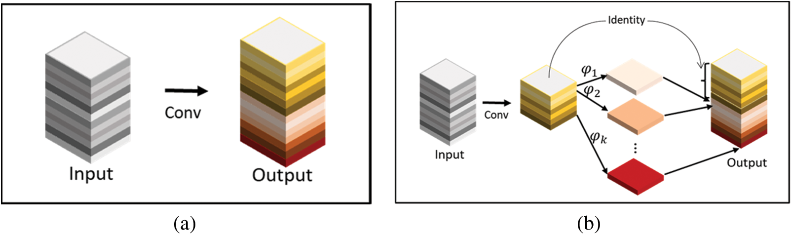
Figure 4: Traditional Conv (a) and GhostConv (b) processing procedure

In the formulas, Y′∈Rh′×w′×m′, * denotes the convolution operation, m is the number of channels for regular convolution, and ϕi,j represents the economical linear transformation convolution operation. Here m<n, and if m=n, it is equivalent to regular convolution.

This method reduces the learning cost of non-critical features by combining a small number of convolutional kernels with more economical linear transformation operations, replacing the conventional convolution approach. This effectively reduces the demand for computational resources without compromising the performance of the YOLOv7 model. In this context, the Ghost module employs depth-wise convolution as a more cost-effective linear transformation [26]. The grouped convolution eliminates inter-channel correlations, ensuring that the current channel features are only related to themselves. On the one hand, this simulates the generation of redundant features, and on the other hand, it significantly reduces the number of parameters and computational load. The structural diagram is illustrated in Fig. 5.

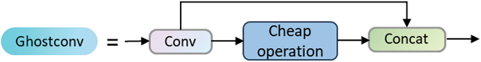
Figure 5: Ghostconv module

2.1.4 The Neck Structure Improvement-Slim Paradigm

In the field of autonomous driving, the Slim-Neck paradigm design has shown excellent performance, and target detection in autonomous driving requires high recognition speed and accuracy of the model [27]. Considering the focus of this paper on water surface target detection, which is intended for real-time detection in maritime applications, there is a similar high requirement for recognition speed and accuracy. Therefore, this paper incorporates the Slim-Neck paradigm design into the YOLOv7 network model.

Currently, lightweight designs primarily rely on Depthwise Separable Convolution (DSC) operations to reduce the number of parameters and FLOPs, mitigating high computational costs. However, when processing DSC input images, channel information is handled separately, leading to significantly lower feature extraction and fusion capabilities compared to standard convolutions (SC). This results in decreased detection accuracy. To address this issue, Li et al. [28] propose a new convolution-GSConv, which employs dense convolution operations to reduce computational costs while maintaining accuracy. As shown in Fig. 6, GSConv better balances the model’s accuracy and speed, and a Slim-Neck structure is designed to enhance CNN learning capabilities.

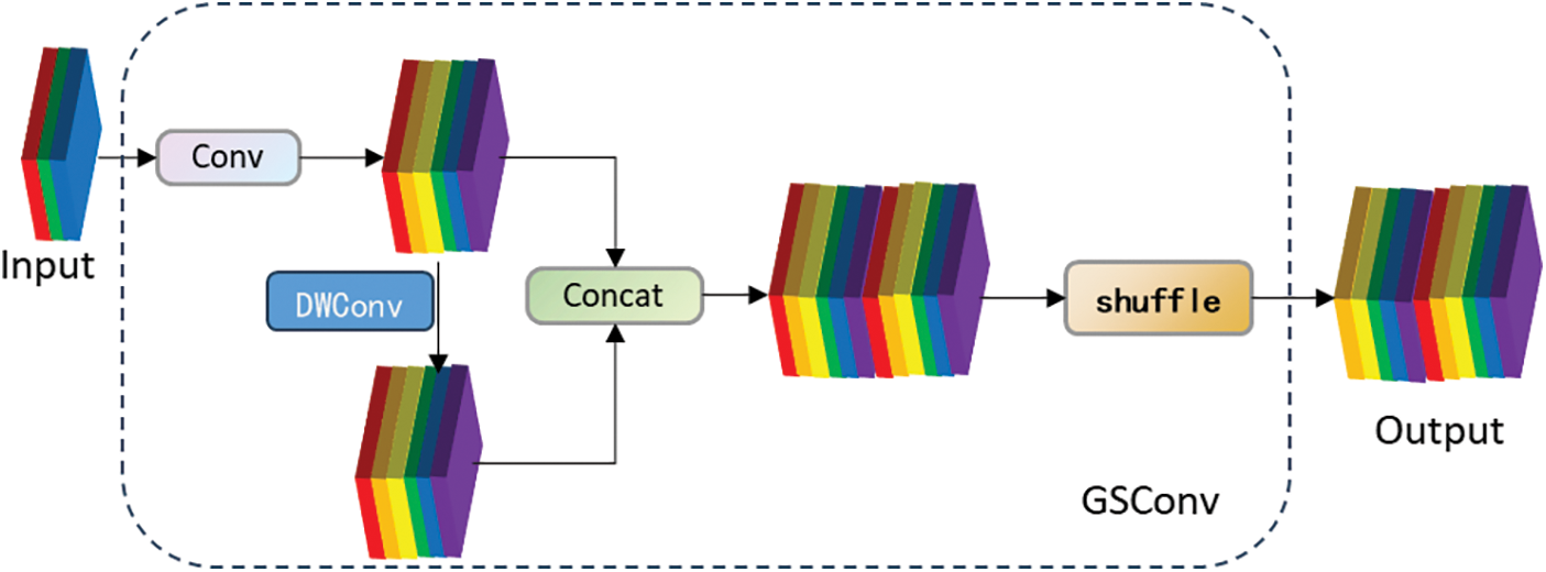
Figure 6: The structure of the GSConv module

However, using GSConv instead of the SC incurs a computational cost of approximately 60% to 70% of SC, with little difference in the model’s learning capabilities compared to the latter. Therefore, based on GSConv, the GSbottleneck is introduced. Similarly, a one-shot aggregation method is used to design the Cross-Stage Partial Network (GSCSP) module, referred to as VoV-GSCSP. The structural diagram is illustrated in Fig. 7. It is worth noting that the VoV-GSCSP module, replaces the Cross Stage Partial Network (CSP) layer in the Neck structure. The CSP layer is made up of standard convolution, resulting in an average reduction of FLOPs by 15.72% compared to the latter. This reduction in FLOPs decreases the complexity of computation and network structure while maintaining sufficient accuracy. Therefore, in this paper, the modules in the original Slim-Neck paradigm structure are replaced with GhostConv, GSbottleneck, and VoV-GSCSP to construct a Slim-Neck structure suitable for this model.

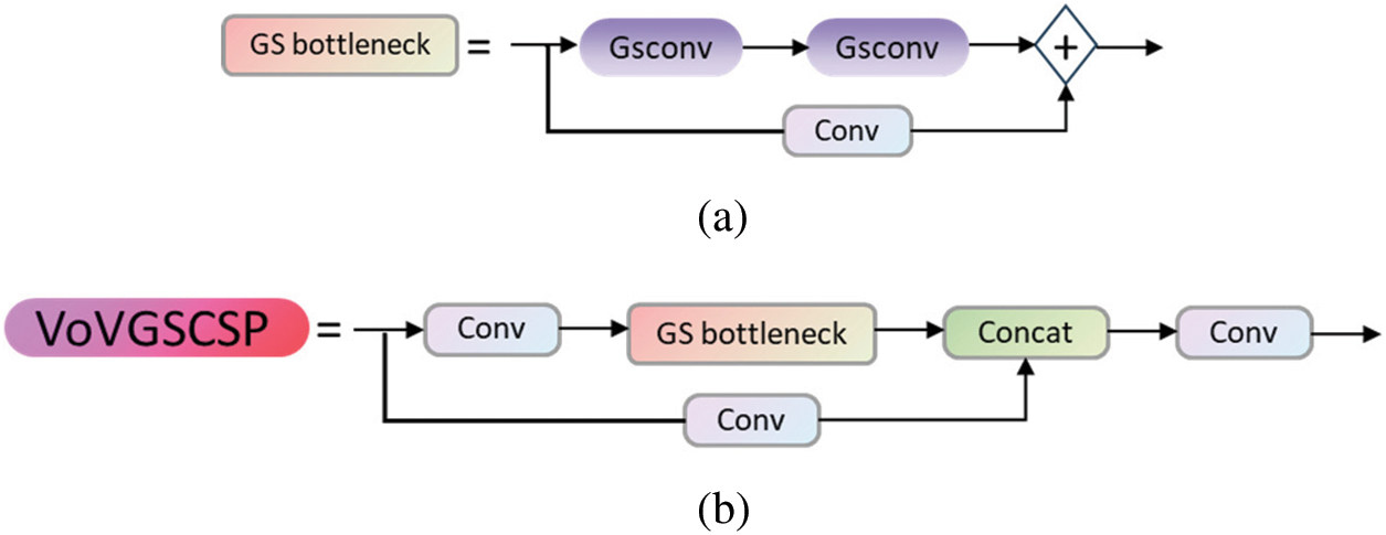
Figure 7: The structure of GS bottleneck module (a) and VoV-GSCSP module (b)

2.1.5 MPDIoU Loss Function

The loss in object detection models is divided into three parts: target confidence loss, classification loss, and coordinate loss. The YOLOv7 model uses binary cross-entropy loss functions for both classification and target confidence losses. The coordinate loss is based on the CIoU loss function, which is founded on the Intersection over Union (IoU) function [29]. The principles of the CIoU loss function are represented by the following formulas [30]:

V=4π2(arctanwgthgt−arctanWprdhprd)2(3)

α={0IoU<0.5V(1−IoU)+VIoU≥0.5(4)

LOSSCloU=1−IoU+ρ2(Bgt,Bprd)c2+αv(5)

In the formulas, wgt, hgt represent the width and height of the ground truth bounding box, while wprd, hprd represent the width and height of the predicted bounding box. V is primarily used to assess whether the aspect ratio is consistent, α is a balancing parameter, Bprd denotes the predicted bounding box, and Bgt denotes the ground truth bounding box. According to the formula, when the aspect ratio of the ground truth box and the predicted box is equal, V=0. In this case, the CIoU loss function fails to effectively express stability. Although the CIoU loss considers the overlap area, center point distance, and aspect ratio of the bounding box regression, its definition of aspect ratio is relative rather than absolute. Additionally, when the predicted bounding box and the ground truth bounding box have the same aspect ratio but different width and height values, the aforementioned bounding box regression loss function loses effectiveness, which will limit convergence speed and accuracy. In this paper, to further improve the robustness of the network, the coordinate loss function of the YOLOv7 model is optimized. The proposed optimization involves replacing YOLOv7’s native CIoU loss function with the MPDIoU loss function [31]. The principal formula of MPDIoU is as follows:

d12=(x1prd−x1gt)2+(y1prd−y1gt)2d22=(x2prd−x2gt)2+(y2prd−y2gt)2(6)

MPDIoU=IoU−d12h2+w2−d22h2+w2 ℒMPDIoU=1−MPDIoU(7)

Based on the above formula and Fig. 8, it can be observed that the MPDIoU loss function is a boundary box regression loss function based on the minimum point distance. Its purpose is to directly minimize the distances between the upper-left and lower-right points of the predicted bounding box and the ground truth bounding box. Compared to the CIoU loss function, the MPDIoU loss function not only considers all factors of the CIoU loss function but also addresses the issue when the predicted bounding box and the ground truth bounding box have the same aspect ratio. This leads to faster convergence speed and more accurate regression results. Moreover, when the predicted bounding box matches the aspect ratio of the ground truth bounding box, the ℒMPDIoU values of the predicted bounding boxes within the ground truth bounding box are lower than those outside. This property ensures the accuracy of bounding box regression and minimizes redundancy in predicted bounding boxes.

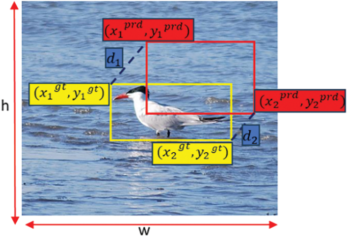
Figure 8: Factors of ℒMPDIoU

2.1.6 The Slide Loss Function

To address the issue of sample imbalance in our self-built dataset, where there is a large number of soft samples and a small number of hard samples, we introduced the slide loss function [32]. The distinction between simple samples and hard samples is based on the IoU between the predicted bounding box and the ground truth box. We calculate the average IoU value for all bounding boxes and use it as a threshold μ. Bounding boxes with an IoU less than μ are considered negative samples, while those with an IoU greater than μ are considered positive samples. By assigning higher weights to hard samples, the model can optimize and learn more effectively from these samples during training. The slide loss function can be expressed by the following formula (8):

f(x)={1x≤μ−0.1e1−μμ<x<μ−0.1e1−xx≥μ(8)

2.2 Fusion Detection of Camera and LiDAR

The fusion of data between camera and LiDAR sensors essentially involves projecting LiDAR point cloud data onto image data. The entire fusion process requires pre-calibration of the camera’s intrinsic parameters as well as the extrinsic parameters between the camera and LiDAR. This paper employs the chessboard grid method for calibrating the camera’s intrinsic parameters and fulfills the extrinsic calibration between the camera and LiDAR by capturing the coordinates of the four corners of a solid-colored calibration board. The entire calibration model is depicted in the Fig. 9: The LiDAR coordinate system describes the relative position of an object to the LiDAR, represented as [XL,YL,ZL]; the camera coordinate system describes the relative position of an object to the camera, represented as [Xc,Yc,Zc]; and the coordinates of a point in the camera coordinate system on the pixel plane are denoted as (u,v).

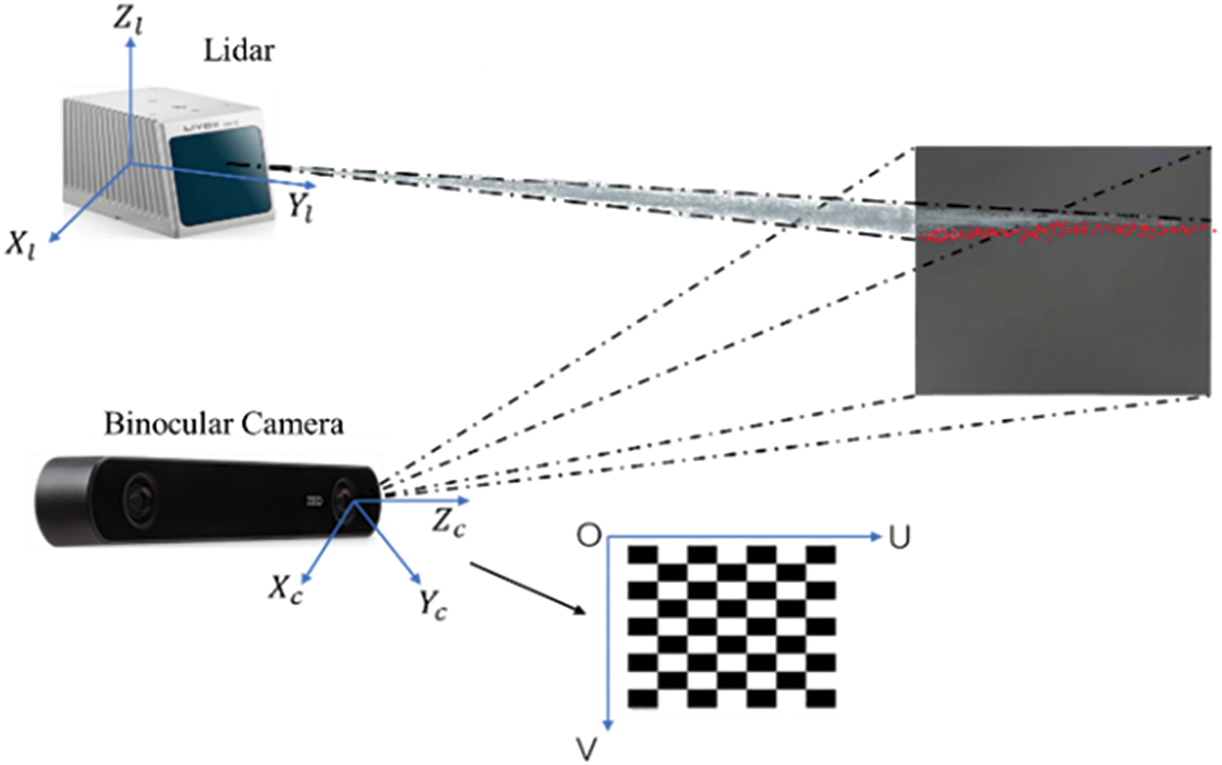
Figure 9: Sensor fusion calibration model

2.2.1 Calibration of Camera Intrinsic Parameters

The calibration process of the camera involves a mathematical transformation between a series of three-dimensional camera coordinates [Xc,Yc,Zc] and their corresponding two-dimensional image pixel points (u,v) to determine the camera’s intrinsic parameters [33]. Essentially, it is a process of finding the transformation relationship from the camera coordinate system to the image coordinate system. This refers to finding the transformation matrix in Eq. (9). dx and dy represent the physical size of the pixels, that is the actual physical size represented by each pixel, and (u0,v0) are the translation offsets between the pixel coordinate system and the physical imaging coordinate system’s origin.

Zc[uv1]=[1/dx0u001/dyu0001][XcYcZc](9)

For the calibration of the camera’s intrinsic parameters in this paper, the image pipeline package within the Robot Operating System (ROS) environment is utilized. Calibration is conducted by launching the camera node, setting the number of corners and dimensions of the chessboard grid, and configuring the camera topic and name before running the calibration command. The chessboard calibration board has corner dimensions of 9 rows × 7 columns, with each square measuring 25 mm × 25 mm. To obtain the best possible calibration result, the chessboard should be moved to various positions and angles within the camera’s field of view. The calibration should continue until the calibrate button becomes active, at which point it can be clicked to compute the intrinsic parameters. The camera intrinsic calibration process is shown in Fig. 10.

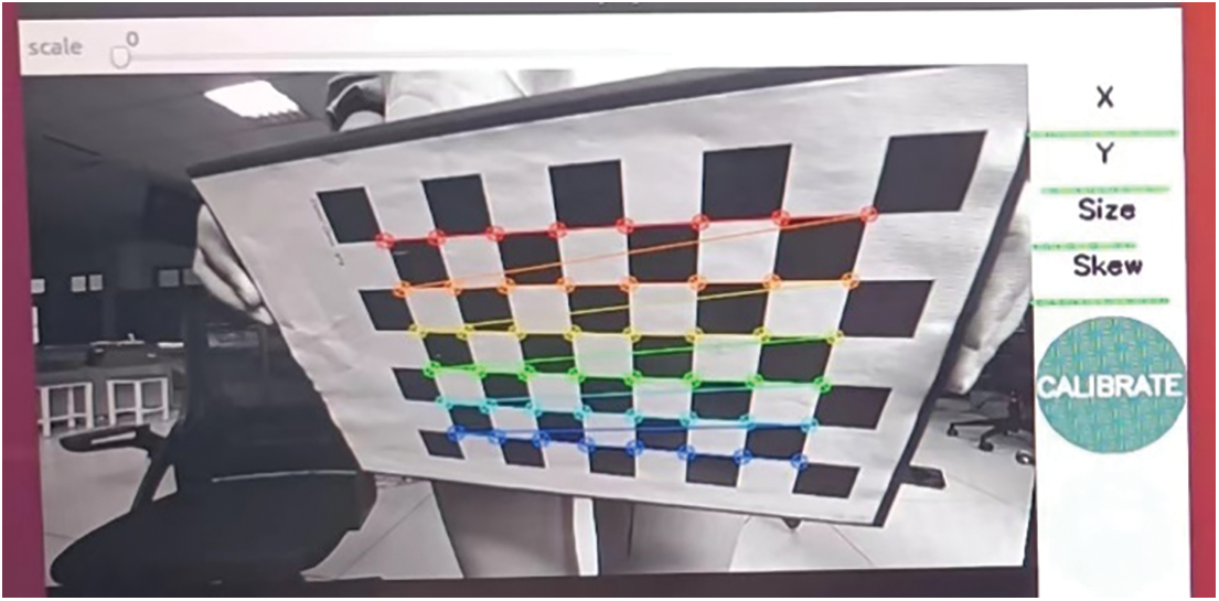
Figure 10: Camera intrinsic parameter calibration process

2.2.2 Calibration of Camera and Lidar External Parameters

The extrinsic calibration between the camera and LiDAR is carried out to obtain the transformation relationship from the LiDAR coordinate system to the camera coordinate system, which involves finding the transformation matrix in Eq. (10). Within this context, R and T represent the rotation matrix and translation matrix between the camera coordinate system and the LiDAR coordinate system, respectively.

[XCYCZC1]=[RT01][XLYLZL1](10)

The extrinsic calibration process involves keeping the positions of the LiDAR and camera static while placing the calibration board at various distances and angles relative to both sensors to collect multiple sets of images and LiDAR point cloud data of the calibration board. This enables the determination of the coordinate relationship between the two sensors. Since the purpose of joint calibration is to use the coordinates of the four corners of the calibration board to obtain the extrinsic parameters, the calibration board should ideally be of a low reflectivity and uniform color [34]. This makes it easier to locate the calibration board’s corners within the LiDAR point cloud data, facilitating the subsequent acquisition of corner coordinates. Limited by experimental conditions, this paper utilized a plain-colored cardboard box as the calibration board, and 16 sets of data were collected from different directions and angles using both the camera and the LiDAR. The corner coordinates of the image data were obtained using Labelimg, while the LiDAR point cloud data coordinates were obtained using Point Cloud Library (PCL) viewer. The resulting images are depicted in the Fig. 11.

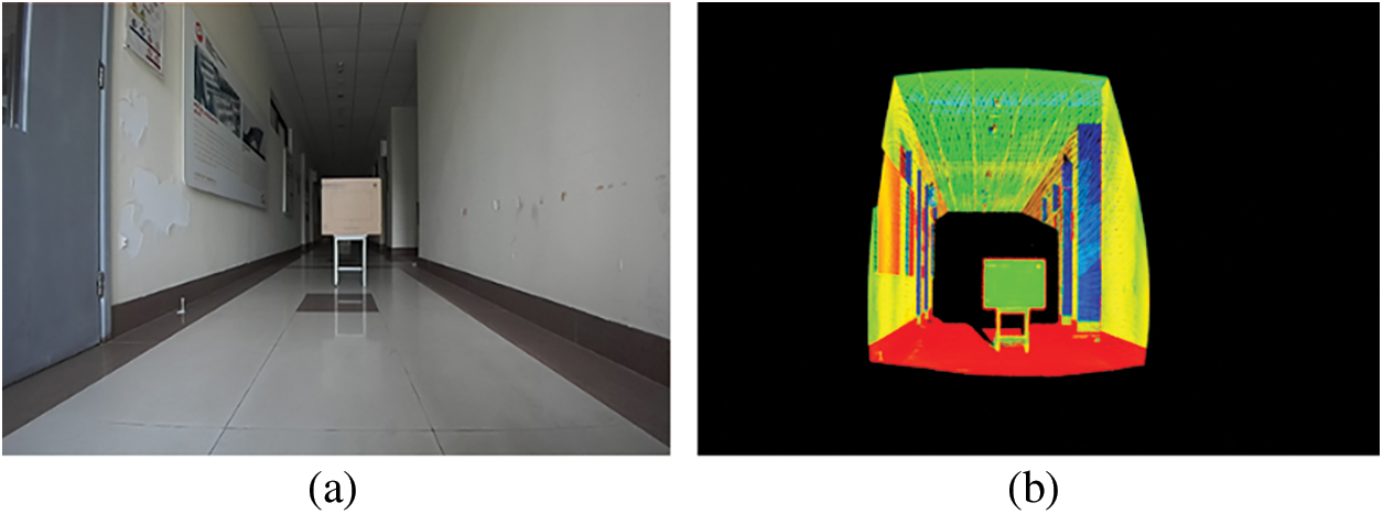
Figure 11: Extrinsic calibration process of camera and LiDAR ((a) Image data (b) LiDAR data)

2.2.3 Camera and LiDAR Data Fusion

Eqs. (9) and (10) provide the transformation relationships from the camera coordinate system to the image coordinate system, and from the LiDAR coordinate system to the camera coordinate system, respectively. To achieve the projection of LiDAR point cloud data onto image data as required by this paper, the transformation relationship from the LiDAR coordinate system to the image coordinate system can be derived by combining the above two coordinate transformation relationships, thereby enabling the point cloud projection effect. The transformation relationship is given by Eq. (11), and the result is depicted in the Fig. 12. The LiDAR used in this paper is a planar LiDAR employing non-repetitive scanning technology, which significantly increases the field-of-view coverage with the increase in integration time.

Figure 12: Fusion results of camera and LiDAR data ((a) Ship image data (b) Ship LiDAR point cloud data (c) Sensor data fusion effect)

ZC[uv1]=[RT][XLYLZL1](11)

3  Experiments

3.1 Experimental Environment and Dataset

The experimental operating system is Ubuntu 20.04, the programming language is Python 3.8.10, and the hardware includes an NVIDIA GeForce RTX 3090 graphics card with 24 GB of memory. The deep learning framework used is PyTorch 1.11.0, and the CUDA version is 11.3. The input image size for the YOLOv7 network model is set to 640 × 640, trained for 150 epochs, with a batch size of 16, and an initial learning rate of 0.01. The sensors used include the Livox Mid-70 LiDAR and the ZED 2i binocular camera. Fig. 13 shows the sensor joint calibration platform.

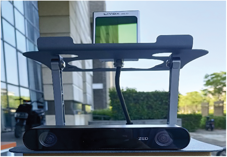
Figure 13: The sensor joint calibration platform

This dataset was collected by combining web crawling and self-collection methods, covering ten classes of potential water surface targets: Sailboat, cruise ship, warship, yacht, cargo ship, other boats, person, airplane, bird and fish, totaling 12316 images. These images were annotated using Labelimg and then divided into training, validation, and test sets with a ratio of 0.7:0.15:0.15. This partition was done to facilitate the training, validation, and testing of the algorithm. The dataset includes targets of various sizes, making it significant for research on USV target detection and obstacle avoidance techniques. Part of the dataset is shown in Fig. 14.

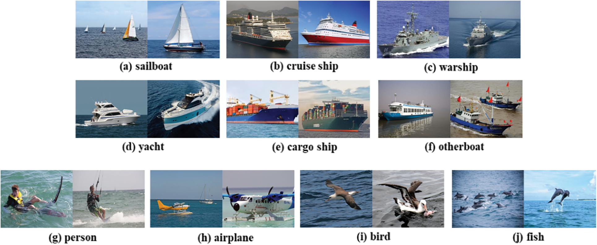
Figure 14: Partial dataset images

3.2 Evaluation Metrics

The evaluation criteria utilized in this paper comprise precision, recall, Frames Per Second (FPS), Giga Floating Point Operations Per Second (GFLOPs) and mean Average Precision (mAP). The calculation formulas are as follows:

P=TPTP+FP×100%(12)

R=TPTP+FN×100%(13)

AP=∫P(R)dR(14)

mAP=1n∑i=1nAPi(15)

In the formulas, TP represents the number of samples that are actual positives and predicted as positives by the model algorithm; FP represents the number of samples that are actual negatives and predicted as positives by the model algorithm; FN represents the number of samples that are actual positives and predicted as negatives by the model algorithm. P is precision; R is recall; AP is average precision, and taking the average of AP values for all categories gives mAP. mAP@0.5 represents the average detection accuracy at an IoU threshold of 0.5 for all target categories. mAP@0.5:0.95 represents the average detection accuracy across 10 IoU thresholds ranging from 0.5 to 0.95 with a step size of 0.05.

3.3 Visual Results Analysis

3.3.1 Ablation Experiments and Data Analysis

In this paper, YOLOv7 is employed as the baseline for surface target detection. Various improvement strategies are then added to this baseline for ablation experiments. Through these ablation experiments, the impact of each improvement component on the target detection model is evaluated and analyzed. The results of the ablation experiments are presented in Table 1.

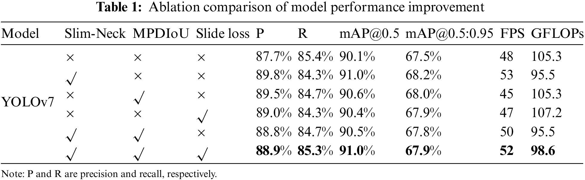
The comparative data presented in Table 1 were obtained from experiments conducted on a proprietary dataset. As indicated by the table, the integration of the Slim-Neck structure into the YOLOv7 model resulted in an increase of 0.9% in mAP@0.5 and 0.7% in mAP@0.5:0.95, while also enhancing the detection speed as measured by FPS, and reducing the model’s computational demand by 9.3% in terms of GFLOPs. A similar improvement in accuracy was observed when either MPDIoU or slide loss was incorporated individually. The concurrent incorporation of the Slim-Neck structure and MPDIoU loss function led to 0.5% decrease in mAP compared to the sole modification of the neck section; however, as demonstrated in Fig. 15, the replacement of the CIoU loss function with MPDIoU resulted in lower loss values during network convergence and a more rapid convergence rate, effectively enhancing the robustness of the YOLOv7 model. Training the improved YOLOv7 model with the dataset yielded results as depicted in Fig. 16, indicating an across-the-board improvement in detection accuracy for various object categories, with the sailing boat category, in particular, achieving an impressive AP of 97.3%. The model’s overall mAP was computed to be 91%.

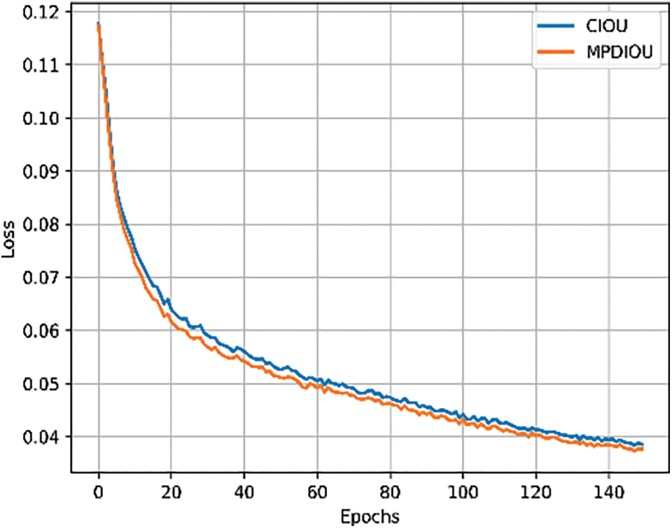
Figure 15: Loss function comparison chart

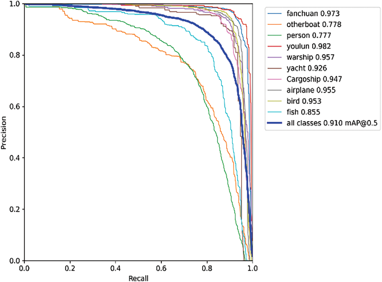
Figure 16: The precision-recall curve of the improved YOLOv7 model

3.3.2 Comparative Analysis with Mainstream Algorithms

In this paper, to verify the superiority of the proposed algorithm, a comparative experiment was conducted by comparing the algorithm with various state-of-the-art algorithms, ensuring consistent configuration environments and initial training parameters. The comparative experiment with mainstream algorithms is presented in Table 2.

From Table 2, it is evident that the improved YOLOv7 model achieves the highest values for mAP, Precision, and Recall compared to other mainstream algorithms. The mAP@0.5 reaches 91%, representing a 0.9% improvement over the original YOLOv7 model and a significant enhancement over SSD, YOLOv5, and YOLOv8 by 14%, 3.2%, and 4%, respectively. As depicted in Fig. 17, the mAP values of the improved YOLOv7 algorithm consistently surpass those of other mainstream algorithms, demonstrating superior performance in water surface target detection. The enhanced YOLOv7 network model exhibits superior capabilities, enhancing both the speed and accuracy of water surface target detection.

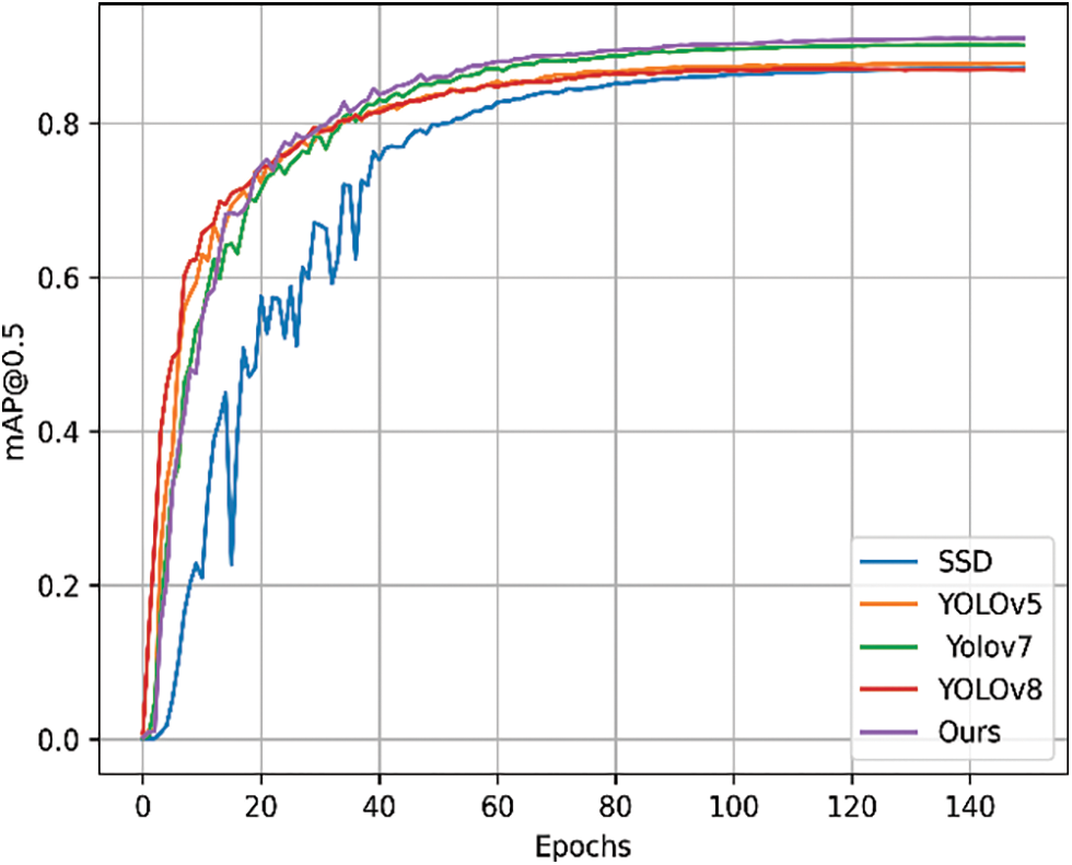
Figure 17: The mAP comparison chart of different mainstream algorithms

3.4 Sensor Fusion Result Analysis

The sensor data fusion experiment involved calibrating the extrinsic parameters between the Livox LiDAR and ZED camera using multiple sets of data based on the coordinates of black calibration board corner points. The optimization process was conducted simultaneously. Additionally, the experiment utilized the camera’s intrinsic parameters obtained through chessboard calibration to achieve the projection of LiDAR point-clouds onto images. The specific parameters are outlined in the Tables 3 and 4.

3.5 Analysis of Experimental Results

For a more intuitive and convenient comparison of the improved YOLOv7 network model, incorporating LiDAR point-cloud fusion, with the original YOLOv7 network model in terms of detection performance, real-time sensor data was collected within the school premises to detect vessels and people. Fig. 18a displays the detection results of the original YOLOv7 model, while Fig. 18b showcases the results of the fused LiDAR point-cloud and the improved YOLOv7 network model. It is evident that the improved model achieves higher accuracy. Additionally, projecting the lidar point-cloud onto the images allows for a clear indication of the target count, addressing issues of omission in purely visual algorithms. Moreover, in the unique environment of the water surface, factors such as target reflections and refractions may occur. Leveraging the LiDAR’s capability to avoid returning data in transparent media, this method effortlessly resolves a range of challenges introduced by complex water surface conditions.

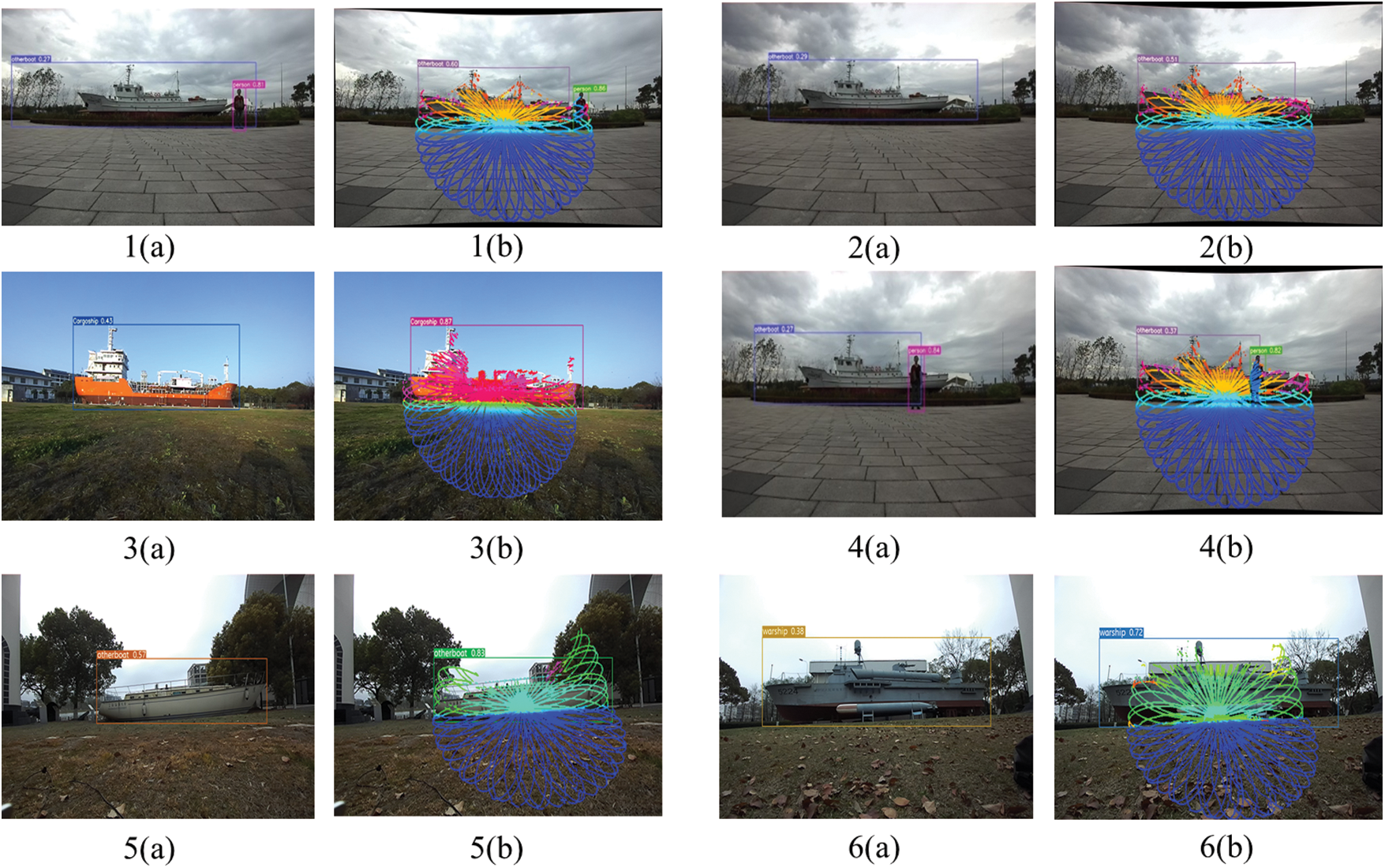
Figure 18: Detection results of YOLOv7 (a) and Our algorithm (b) (Our algorithm is based on the improved YOLOv7 for sensor fusion detection)

4  Conclusion

In this paper, in addressing the challenges of water surface target detection, including missed detections, false positives, and low detection rates in complex water environments using purely visual algorithms, a method integrating visual and LiDAR sensor data is proposed. For the visual sensor component, improved YOLOv7 algorithm is employed to improve detection rates and enhance model robustness. Firstly, a lightweight Slim-Neck paradigm structure is designed by introducing the GhostConv module and VOV-GSCSP module, addressing the issue of redundancy in feature extraction while reducing the complexity of the network model. Secondly, to tackle the problem of slow model convergence, the MPDIoU loss function replaces the original CIoU loss function, enhancing the model’s robustness. Finally, to address the issue of imbalance in the self-built dataset, the slide loss function is introduced to enable the model to optimize learning from these samples. The algorithms proposed in this paper have improved target detection accuracy compared to mainstream algorithms, reaching 91%. For the LiDAR sensor component, leveraging the point-cloud reflection characteristics of LiDAR in water media, an approach is adopted to jointly calibrate the LiDAR and camera by obtaining the extrinsic parameters. This is complemented by internal camera calibration to project LiDAR point-clouds onto images, refining the detection of targets in the challenging and complex environment of water surfaces.

Acknowledgement: We thank all the members who have contributed to this work with us.

Funding Statement: The paper is supported by the National Natural Science Foundation of China (No. 51876114) and the Shanghai Engineering Research Center of Marine Renewable Energy (Grant No. 19DZ2254800).

Author Contributions: Study conception and design: Yongguo Li, Yuanrong Wang; data collection: Caiyin Xu, Kun Zhang; analysis and interpretation of results: Jia Xie, Yuanrong Wang; draft manuscript preparation: Yuanrong Wang. All authors reviewed the results and approved the final version of the manuscript.

Availability of Data and Materials: The data that support the findings of this study are available from the second author upon reasonable request.

Conflicts of Interest: The authors declare that they have no conflicts of interest to report regarding the present study.

References

1. T. K. Behera, S. Bakshi, M. A. Khan, and H. M. Albarakati, “A lightweight multiscale-multiobject deep segmentation architecture for UAV-based consumer applications,” IEEE Trans. Consum. Electron., vol. 70, pp. 1, 2024. doi: 10.1109/TCE.2024.3367531. [Google Scholar] [CrossRef]

2. J. M. Larrazabal and M. S. Peñas, “Intelligent rudder control of an unmanned surface vessel,” Expert Syst. Appl., vol. 55, pp. 106–117, Aug. 2016. doi: 10.1016/j.eswa.2016.01.057. [Google Scholar] [CrossRef]

3. L. Cheng et al., “Water target recognition method and application for unmanned surface vessels,” IEEE Access, vol. 10, pp. 421–434, 2022. doi: 10.1109/ACCESS.2021.3138983. [Google Scholar] [CrossRef]

4. L. Ren, Z. Li, X. He, L. Kong, and Y. Zhang, “An underwater target detection algorithm based on attention mechanism and improved YOLOv7,” Comput. Mater. Contin., vol. 78, no. 2, pp. 2829–2845, 2024. doi: 10.32604/cmc.2024.047028. [Google Scholar] [CrossRef]

5. Y. Lecun, L. Bottou, Y. Bengio, and P. Haffner, “Gradient-based learning applied to document recognition,” in Proc. IEEE, Nov. 1998, vol. 86. no. 11. pp. 2278–2324. doi: 10.1109/5.726791. [Google Scholar] [CrossRef]

6. W. Wu, X. Li, Z. Hu, and X. Liu, “Ship detection and recognition based on improved YOLOv7,” Comput. Mater. Contin., vol. 76, no. 1, pp. 489–498, 2023. doi: 10.32604/cmc.2023.039929. [Google Scholar] [CrossRef]

7. Q. Zhu, K. Ma, Z. Wang, and P. Shi, “YOLOv7-CSAW for maritime target detection,” Front Neurorob., vol. 17, pp. 1210470, Jul. 2023. doi: 10.3389/fnbot.2023.1210470. [Google Scholar] [PubMed] [CrossRef]

8. A. Stateczny, W. Kazimierski, D. Gronska-Sledz, and W. Motyl, “The empirical application of automotive 3D radar sensor for target detection for an autonomous surface vehicle’s navigation,” Remote Sens., vol. 11, no. 10, pp. 10, Jan. 2019. doi: 10.3390/rs11101156. [Google Scholar] [CrossRef]

9. J. Wang and F. Ma, “Obstacle recognition method for ship based on 3D lidar,” in 2021 6th Int. Conf. Transp. Inform. Safety (ICTIS), Wuhan, China, IEEE, Oct. 2021, pp. 588–593. doi: 10.1109/ICTIS54573.2021.9798671. [Google Scholar] [CrossRef]

10. X. Qi, W. Fu, P. An, B. Wu, and J. Ma, “Point cloud preprocessing on 3D LiDAR data for unmanned surface vehicle in marine environment,” in 2020 IEEE Int. Conf. Inform. Technol., Big Data Artif. Intell. (ICIBA), Nov. 2020, pp. 983–990. doi: 10.1109/ICIBA50161.2020.9277346. [Google Scholar] [CrossRef]

11. J. Zhou, P. Jiang, A. Zou, X. Chen, and W. Hu, “Ship target detection algorithm based on improved YOLOv5,” J. Mar. Sci. Eng., vol. 9, no. 8, pp. 908, Aug. 2021. doi: 10.3390/jmse9080908. [Google Scholar] [CrossRef]

12. J. Han, Y. Liao, J. Zhang, S. Wang, and S. Li, “Target fusion detection of LiDAR and camera based on the improved YOLO algorithm,” Mathematics, vol. 6, no. 10, pp. 213, Oct. 2018. doi: 10.3390/math6100213. [Google Scholar] [CrossRef]

13. Z. Lu, B. Li, and J. Yan, “Research on unmanned surface vessel perception algorithm based on multi-sensor fusion,” in 2022 4th Int. Conf. Front. Technol. Inform. Comput. (ICFTIC), Qingdao, China, IEEE, Dec. 2022, pp. 286–289. doi: 10.1109/ICFTIC57696.2022.10075187. [Google Scholar] [CrossRef]

14. L. Wang, Y. Xiao, B. Zhang, R. Liu, and B. Zhao, “Water surface targets detection based on the fusion of vision and LiDAR,” Sensors, vol. 23, no. 4, pp. 1768, Feb. 2023. doi: 10.3390/s23041768. [Google Scholar] [PubMed] [CrossRef]

15. C. Y. Wang, A. Bochkovskiy, and H. Y. M. Liao, “YOLOv7: Trainable bag-of-freebies sets new state-of-the-art for real-time object detectors,” presented at the Proc. IEEE/CVF Conf. Comput. Vis. Pattern Recognit., 2023, pp. 7464–7475. doi: 10.1109/CVPR52729.2023.00721. [Google Scholar] [CrossRef]

16. G. Jocheret al., “ultralytics/yolov5: V5.0-YOLOv5-P6 1280 models, AWS, Supervise.ly and YouTube integrations,” Zenodo, Apr. 2021. doi: 10.5281/zenodo.4679653. [Google Scholar] [CrossRef]

17. Z. Ge, S. Liu, F. Wang, Z. Li, and J. Sun, “YOLOX: Exceeding YOLO series in 2021,” Aug. 05, 2021. doi: 10.48550/arXiv.2107.08430. [Google Scholar] [CrossRef]

18. C. Y. Wang, I. H. Yeh, and H. Y. M. Liao, “You only learn one representation: Unified network for multiple tasks,” May 10, 2021. doi: 10.48550/arXiv.2105.04206. [Google Scholar] [CrossRef]

19. X. Ding, X. Zhang, N. Ma, J. Han, G. Ding and J. Sun, “RepVGG: Making VGG-style ConvNets great again,” presented at the Proc. IEEE/CVF Conf. Comput. Vis. Pattern Recognit., 2021. Accessed: Dec. 26, 2023. [Online]. Available: https://openaccess.thecvf.com/content/CVPR2021/html/Ding_RepVGG_Making_VGG-Style_ConvNets_Great_Again_CVPR_2021_paper.html [Google Scholar]

20. S. Han, J. Pool, J. Tran, and W. Dally, “Learning both weights and connections for efficient neural network,” in Adv. Neural Inform. Process. Syst., 2015. Accessed: Dec. 28, 2023. [Online]. Available: https://proceedings.neurips.cc/paper/2015/hash/ae0eb3eed39d2bcef4622b2499a05fe6-Abstract.html [Google Scholar]

21. M. Courbariaux, Y. Bengio, and J. P. David, “BinaryConnect: Training deep neural networks with binary weights during propagations,” in Adv. Neural Inform. Process. Syst., 2015. Accessed: Dec. 28, 2023. [Online]. Available: https://proceedings.neurips.cc/paper_files/paper/2015/hash/3e15cc11f979ed25912dff5b0669f2cd-Abstract.html [Google Scholar]

22. G. Hinton, O. Vinyals, and J. Dean, “Distilling the knowledge in a neural network,” Mar. 09, 2015. doi: 10.48550/arXiv.1503.02531. [Google Scholar] [CrossRef]

23. A. G. Howard et al., “MobileNets: Efficient convolutional neural networks for mobile vision applications,” Apr. 16, 2017. doi: 10.48550/arXiv.1704.04861. [Google Scholar] [CrossRef]

24. X. Zhang, X. Zhou, M. Lin, and J. Sun, “ShuffleNet: An extremely efficient convolutional neural network for mobile devices,” Dec. 07, 2017. doi: 10.48550/arXiv.1707.01083. [Google Scholar] [CrossRef]

25. K. Han, Y. Wang, Q. Tian, J. Guo, C. Xu and C. Xu, “GhostNet: More features from cheap operations,” in 2020 IEEE/CVF Conf. Comput. Vis. Pattern Recognit. (CVPR), Seattle, WA, USA, IEEE, Jun. 2020, pp. 1577–1586. doi: 10.1109/CVPR42600.2020.00165. [Google Scholar] [CrossRef]

26. Q. Han et al., “On the connection between local attention and dynamic depth-wise convolution,” Aug. 04, 2022. doi: 10.48550/arXiv.2106.04263. [Google Scholar] [CrossRef]

27. J. D. Choi and M. Y. Kim, “A sensor fusion system with thermal infrared camera and LiDAR for autonomous vehicles and deep learning based object detection,” ICT Express, vol. 9, no. 2, pp. 222–227, Apr. 2023. doi: 10.1016/j.icte.2021.12.016. [Google Scholar] [CrossRef]

28. H. Li, J. Li, H. Wei, Z. Liu, Z. Zhan and Q. Ren, “Slim-neck by GSConv: A better design paradigm of detector architectures for autonomous vehicles,” J. Real-Time Image Proc., vol. 21, no. 3, pp. 62, May 2024. doi: 10.1007/s11554-024-01436-6. [Google Scholar] [CrossRef]

29. J. Yu, Y. Jiang, Z. Wang, Z. Cao, and T. Huang, “UnitBox: An advanced object detection network,” in Proc. 24th ACM Int. Conf. Multimed., New York, NY, USA, Association for Computing Machinery, Oct. 2016, pp. 516–520. doi: 10.1145/2964284.2967274. [Google Scholar] [CrossRef]

30. Z. Zheng et al., “Enhancing geometric factors in model learning and inference for object detection and instance segmentation,” IEEE Trans. Cybern., vol. 52, no. 8, pp. 8574–8586, Aug. 2022. doi: 10.1109/TCYB.2021.3095305. [Google Scholar] [PubMed] [CrossRef]

31. M. Siliang and X. Yong, “MPDIoU: A loss for efficient and accurate bounding box regression,” 2023. doi: 10.48550/arXiv.2307.07662. [Google Scholar] [CrossRef]

32. Z. Yu, H. Huang, W. Chen, Y. Su, Y. Liu and X. Wang, “YOLO-FaceV2: A scale and occlusion aware face detector,” 2022. doi: 10.48550/arXiv.2208.02019. [Google Scholar] [CrossRef]

33. Z. Zhang, “A flexible new technique for camera calibration,” IEEE Trans. Pattern Anal. Mach. Intell., vol. 22, no. 11, pp. 1330–1334, Nov. 2000. doi: 10.1109/34.888718. [Google Scholar] [CrossRef]

34. Y. Yu, S. Fan, L. Li, T. Wang, and L. Li, “Automatic targetless monocular camera and LiDAR external parameter calibration method for mobile robots,” Remote Sens., vol. 15, no. 23, pp. 23, Jan. 2023. doi: 10.3390/rs15235560. [Google Scholar] [CrossRef]