A Prediction-Based Multi-Objective VM Consolidation Approach for Cloud Data Centers

1  Introduction

Cloud computing is a computational paradigm that offers its users scalable services in an on-demand pattern. The most prominent feature of cloud computing is that it provides users with virtualized resources [1]. Cloud computing utilizes various technologies, such as virtualization, distributed computing, and storage. It eliminates front-end capital and customers’ ongoing maintenance. Cloud computing permits customers to increase and decrease resource demands and pay accordingly [2]. Cloud providers (CPs) should allocate and deallocate resources on demand. As a result, operating costs are reduced [3].

VM consolidation can improve the utilization of resources by reducing EC in cloud data centers [4]. VM consolidation process consists of three phases in general [4]:

1.    Detection of overload/underload PMs. Identifying overloaded PMs and migrating VMs to prevent potential PD or even Service Level Agreements (SLA) violations. Identifying underloaded PMs, migrating all VMs on the PMs, and turning the PMs off to reduce EC.

2.    VM selection. The candidate VMs from overload PMs are selected to keep the PM under average load. Some policies, such as Maximum Correlation Coefficient (MCC), Minimum Migration Time (MMT), and Minimum Utilization (MU) are utilized.

3.    PM selection. The destination PMs for the VMs coming from overload/underload PMs. Some objectives, such as EC, RW, and MC, can be considered.

Most works consolidate VMs based on PM/VM current resource utilization. In other words, all three phases of VM consolidation should be performed based on current resource utilization. However, due to the unsteadiness and high changeability of the workload, PM/VM resource utilization is unstable and highly variable. Improving these three phases of VM consolidation is essential to matching VM’s dynamic change of workload and resource capacity. The first phase of VM consolidation requires an approach that predicts future resource usage. Otherwise, the detection results of overload/underload will soon become invalid, and a high number of needless VM migrations may be caused not only because the workload is highly variable but also because there are large numbers of PMs and VMs in the data center, it takes neglected time to make and implement migration decisions. For instance, according to a migration decision, a VM should be migrated from an overload PM to another underload PM. Unfortunately, this underload PM cannot accommodate the VM when implementing the migration decision due to real-time changes in workload. The unreliable detection result in the first phase may result in the selected VMs and destination PMs not being the optimal options in the second and third phases. The unreliable detection result increases the overheads, such as the EC for VM migration, PD, and network traffic [5,6].

On the other hand, the existing works consider a few optimization goals. The obtained consolidation solutions may need to be improved in other optimization goals and hinder their application in practice. It is essential to consider more goals while consolidating VMs, as more factors influence the quality of the consolidation solution in practice:

Although VM migration can reduce EC, VM migration also gives rise to VM PD or SLA violation on new PMs because sharing hardware resources among more VMs increases resource contention.

The MC of a VM in different cloud data centers varies greatly because it is heavily dependent on data center’s configuration, such as network architecture and bandwidth usage, and the application executed on the VM.

Maximizing resource utilization has always been an essential resource management goal in data centers.

The above considerations may be conflicting when combined. Therefore, finding an effective strategy that considers compromise among all the goals is essential.

This paper introduces a novel prediction-based multi-objective VM consolidation approach that stands out for its two key innovations. The first innovation is a hybrid method that combines ARIMA and SVR to predict future resource usage. The second innovation is the consideration of multiple objectives such as EC, PD, MC, and RW, and the optimization of these objectives using Nsga2 based on future resource utilization. This approach allows for the search for the optimal solution in a more timely and practical manner.

The main contributions of this paper are summarized as follows:

1.    We propose a prediction approach based on the ARIMA-SVR model to forecast future VM resource demand, which can capture both linear and nonlinear features of resource demand data. Specifically, we use the ARIMA model to predict the future resource demand of VM preliminarily. Because the ARIMA model can only capture linear time series features, we use the SVR model to assist the ARIMA model. The SVR model predicts future errors. Adding the forecasts of the ARIMA and SVR models obtains the final prediction.

2.    We design a framework to predict future resource demands of VMs in a cloud data center. This framework depicts the process for predicting future VM resource demand. We propose an algorithm to estimate the parameters of the SVR model and train it.

3.    Our proposed prediction-based multi-objective VM consolidation approach, which leverages future resource demands of VMs for multi-objective optimization, offers significant practical value. It enables the obtained consolidation solution to be both timely and practical. To validate the effectiveness of our approach, we have conducted a series of rigorous experiments.

We organize this paper as follows: Section 2 reviews the related works on resource usage prediction in cloud data centers and multi-objective VM consolidation. Section 3 provides our problem formulation. Section 4 provides the specifics of the proposed approach, including the prediction framework and algorithms. Section 5 is devoted to performance evaluation and shows the superiority of the proposed approach. We conclude the paper and describe future work in Section 6.

2  Related Works

2.1 Resource Usage Prediction in Cloud Environment

The VM’s resource demand may change over time. Accurate prediction of VM’s future resource demand improves resource utilization efficiency. Some approaches have been developed to predict cloud resource demand. Reference [7] used a gray model to predict the host’s CPU and RAM resource usage. The gray model does not require a large number of training data. However, it cannot guarantee accurate prediction of workloads with frequent fluctuations. Exploiting a Gray-Markov (G-M)-based model predicts future usage of resources [8]. Reference [9] used a Discrete-Time Markov chain (DTMC) model to predict future resource usage. It presents a multi-objective VM placement approach to search for the optimal solution for the VM placement problem by exploiting the ε-dominance-based multi-objective artificial bee colony (ε-MOABC) algorithm.

Other researchers use machine learning (ML) technology to predict resource usage. Reference [10] proposed a Host States Naive Bayesian Prediction (HSNBP) model in cloud data centers. The HSNBP model can forecast overload hosts using The Naive Bayesian (NB) classifier. Reference [11] proposed an ARIMA model for forecasting workload. Due to the simplicity of implementation, LR was used to estimate future resource usage in many types of research. Reference [12–15] proposed employing LR methods to predict CPU usage. However, the LR technique considers only the linear features in time series data. The relationship between resource demand data and time appears more curved. In [16], the authors replaced the LR with a K-Nearest Neighbor Regression (KNNR). To avoid needless VM migration, reference [17] proposed a Bayesian network-based estimation model for live VM migration. Reference [18] presented a self-directed workload forecasting method (SDWF). SDWF utilizes a Multilayer Neural Network (MNN) to learn historical data and forecast the next possible workload value. Reference [19] presented a Multi-Resource Feed-forward Neural Network (MR-FNN) to predict the multiple resource demands concurrently. MR-FNN uses a differential evolution algorithm to enhance its learning and prediction capability. Reference [2] employed SVR to predict the future usage of multi-attribute host resources. They applied a Sequential Minimal Optimization (SMO) algorithm to train the SVR model. Reference [20] proposed a framework for cloud resource allocation based on reinforcement learning (RL) mechanism and fuzzy logic (FL).

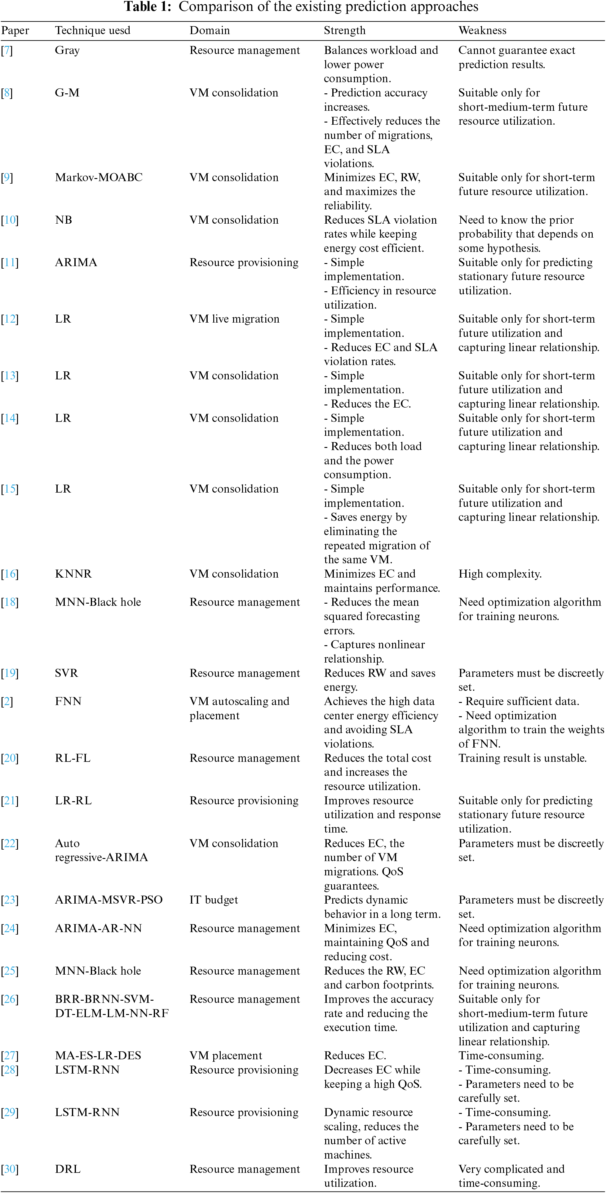
To enhance prediction accuracy, some researchers use hybrid or ensemble learning methods. Reference [21] presented a hybrid method that combines LR and RL techniques to handle changes in workload trace. In [22], host overload detection is based on an ARIMA model. Reference [23] proposed a new Swarm Intelligence Based Prediction Approach (SIBPA) to predict the resource demands of a cloud user. SIBPA combines the Multiple SVRs and ARIMA models to consider mapping the linear and nonlinear attributes in time series. It uses the Particle Swarm Optimization (PSO) approach to select the best features for prediction results. Reference [24] employed ARIMA and Auto-Regressive Neural Network (ARNN) to predict the usage of resources. Reference [3] developed different ML prediction models to perform a consolidation, including LR, Multilayer Perceptron (MLP), SVR, Decision Tree Regression (DTR), and Boosted Decision Regression (BDR). Reference [25] presented an ensemble learning-based workload forecasting method. The proposed framework employs multiple MNNs as base predictors. It used an algorithm illuminated by black hole theory to select the best weight. Reference [26] proposed an Intelligent Regressive Ensemble Approach for Prediction (REAP), which uses eight ML methods to predict CPU usage. Reference [27] proposed an ensemble prediction for forecasting the future needs of resources. The proposed predictor consists of four fundamental prediction models: MA, exponential smoothing (ES), LR, and double ESs. Other researchers use Deep Learning techniques to predict resource usage. Reference [28] proposed a host load predictive model based on a long short-term memory model in a recurrent neural network (LSTM-RNN). Reference [29] developed the workload prediction based on LSTM networks, which uses four LSTMs. Reference [30] proposed a deep RL-based resource management. Table 1 compares all the above prediction approaches regarding application domain, strengths, and weaknesses. These approaches do not consider prediction-based multi-objective optimization. Thus, the issued decision can be insignificant because real-world problems are often multi-objective optimization problems. In this paper, we propose a prediction model based on which we optimize multiple objectives simultaneously. In addition, the proposed prediction model can capture both linear and nonlinear features of resource demand data.

2.2 Multi-Objective VM Consolidation

This section presents the optimization approaches to VM consolidation proposed in existing works. We divide these approaches into categories: (1) multi-objective approach transformed into mono-objective and (2) multi-objective approach.

(1) Multi-objective transformed into mono-objective approach

They combine multiple objectives into a mono-objective. This approach may be classified as I. the weighted sum method. The user gives the weight of each objective. II. the constraint method. Choosing only one objective as mono-objective and considering other objectives as constraints.

I. The weighted sum method

They combine all objectives into a mono-objective by attaching each weight to each objective. A multi-objective energy-efficient VM consolidation using adaptive beetle swarm optimization (ABSO) algorithm is proposed [31]. The proposed ABSO is a hybridization of PSO and BSO. Reference [32] studied consolidation problems of processor-intensive and disk-intensive workloads and formulated the problem as the four-objective functions. The objective functions are (1) total energy consumed by the processor, disk, VM migration and turning PMs ON and OFF, (2) consolidation fitness of multiple disk-intensive VMs, (3) processor utilization of PM on which at least one disk intensive VM is running and (4) number of PMs with too high processor utilization. To solve the presented multi-objective optimization problem, it first calculates the optimum point for each objective, then weights the difference ratios between each objective function and its optimum point and sums them finally. The Simulated Annealing (SA) method obtains the optimal solution. Reference [33] proposed a method based on the Monarch Butterfly Optimization algorithm (MBO) for VM placement to maximize packaging efficiency and reduce the number of active physical servers. Reference [1] aimed at controlling manufacturing costs and treated MCs, the energy cost of servers, the cost of creating VMs, and the total penalty cost for tasks whose demands are not satisfied as four objective functions. The user determines the weights.

The approaches above are all priori methods, and they must clarify prior information’s impacts on their solution. First, it is challenging to set weights accurately. Second, the metric used in calculating the objective function is diverse for diverse objectives, resulting in a significant error in the weighted objective function value.

II. The constraints method

They treat one of the objectives as one objective and consider the others as constraints. Reference [5] minimized the number of the required hosts for hosting VMs under SLA constraint. Reference [34] aimed at reducing the EC, composed of three parts: cost of assigning new VMs to PMs, MC, and cost of keeping PMs turned on, and treated the demands of CPU, memory, and network bandwidth as resource constraints. Reference [35] presented security-aware VM consolidation, which treats reducing the security risk of a PM as an objective, and the risk increase for each VM does not exceed the value of the proposed Risk Increase Threshold (RITH) as a constraint. Reference [36] proposed a failure-aware VM consolidation approach, which regards failures arising as a constraint before performing VM consolidation. Reference [37] presented an Interval-valued Fuzzy Logic (FL) mechanism aiming at power conservation while optimizing performance.

Constraints limit the variation range of independent variables on an objective. The solution obtained by this constraint may differ from the exact solution to that objective.

(2) Multi-objective method

A multi-objective optimization problem includes multiple objective functions and multiple constraints. To compare the two solutions, the concept of Pareto dominance is introduced. Reference [38] proposed a two-objective approach and made a tradeoff between these objectives using a Fuzzy Analytic Hierarchy Process (FAHP). Reference [39] aimed at energy saving and network bandwidth consumption and proposed a two-objective approach that treats the number of the required hosts for hosting VMs and the number of VM migrations as objective functions under SLA constraint. Reference [9] proposed a VM placement approach to obtain the optimal solution using the ε-MOABC algorithm, which can efficiently balance the overall EC, RW, and system reliability. Reference [40] proposed an approach that uses an assembly of sine cosine algorithm (SCA) and ant lion optimizer (ALO) for optimal VM assignment. The three objectives are EC, RW, and SLA levels. Reference [41] proposed a multi-objective ant colony (AC) system algorithm for VM consolidation. The goal is to minimize total RW and EC simultaneously. Reference [42] proposed an energy-aware and QoS-aware multi-objective AC Optimization (ACO) approach for VM consolidation.

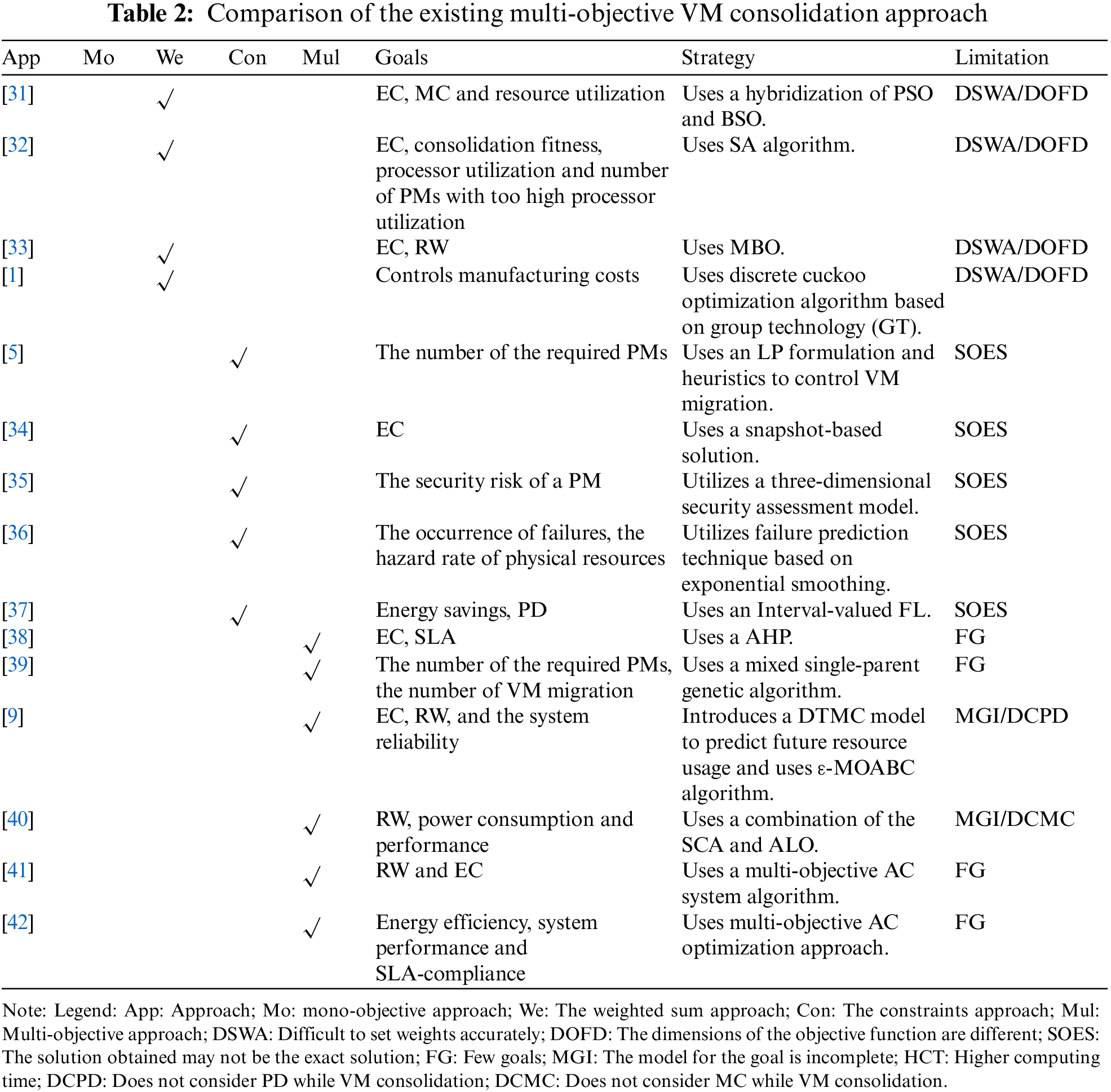
The discussed multi-objective approaches have focused on only two or three factors and treat other factors as constraints, such as SLA. As for the VM consolidation problem, the factors may conflict with each other (i.e., minimizing EC and minimizing SLA violation, etc.). Therefore, each factor should be regarded as an objective instead of a constraint. Table 2 compares the approaches mentioned above.

3  Problem Formulation

3.1 Multi-Objective Optimization Formulation

To consolidate VMs dynamically when resource usage changes, we need to get an optimal allocation between VMs and PMs, which can optimize multiple system goals. Our work uses two-dimensional resources (i.e., CPU and memory) to characterize VMs and PMs because the VM’s image file is stored in network-attached storage (SAN) in VM live migration technology. We propose a prediction-based multi-objective VM consolidation approach that minimizes a data center’s total EC, RW, MC, and PD.

3.1.1 EC Modeling

Our previous work [43] introduced an EC model that considers EC in diverse states, EC of states switching, and EC of live migrations. The model we adopted in this paper significantly contributes to the VM consolidation field. Its inclusion in our research underscores the importance of considering EC in various scenarios, enhancing the robustness and applicability of our approach.

3.1.2 Performance Modeling

We can measure system performance in terms of such characteristics as turnaround time, maximum execution time, and maximum access capacity. It is challenging to evaluate and measure these characteristics directly. More importantly, these characteristics can vary with diverse applications. To assess and measure conveniently, we model PD when SLAV occurs and treat minimizing PD as one of the optimization objectives. We define that the SLA is delivered when 100% of the performance requested by an application inside a VM is provided at any time. As a result, SLA is violated when the system does not fully provide the performance requested by an application inside a VM at some point. There are two cases where the system cannot entirely perform an application request. One is that a PM serving applications is experiencing 100% utilization, and another is a live VM migration is in progress (i.e., it requires a specific MC such as migration latency and downtime). Therefore, we adopt two metrics proposed in [44] to calculate SLAV: SLA violation Time per Active Host (SLATAH) and the overall PD due to VM migrations (PDM).

SLATAH=1N∑i=1NTsiTaiPDM=1M∑j=1MCdjCrj(1)

SLATAH and PDM are calculated with Eq. (1). Where N is the number of PMs, Tsi is the total time during which the ith PM has experienced the utilization of 100%, Tai is the total time during which the ith PM is in the active mode, M is the number of VMs, Cdj is the estimate of the PD of the jth VM caused by migration and Crj is the total CPU capacity requested by the jth VM during its lifetime. From both of the above, SLAV is defined by Eq. (2).

SLAV=SLATAH⋅PDM(2)

The value of SLAV is a real number between 0 and 1, usually expressed as a percentage. A larger value indicates a more severe SLAV.

3.1.3 MC Modeling

MC is highly dependent on data center conditions, such as network architecture, bandwidth usage, the application itself (i.e., how many pages the application updates during migration), and VM memory usage (i.e., memory read or write intensity). MC includes migration latency and downtime.

Migration latency is related to the VM size, workload characteristics, and network transmission rate. All memory pages are copied to the target PM in the pre-copy phase while the VM remains running. During the phase, some pages will be modified many times and must be copied many times to ensure data consistency between source PM and target PM [45]. The continuous formation of dirty pages means that pre-copy should be carried out in several rounds, and the dirty pages to be transmitted during one round should be generated in the previous round. There are four conditions used to terminate iterations: (1) the number of iterations exceeds a pre-defined threshold (n > nth), (2) the total amount of memory transmitted exceeds a given value (m > mth), (3) the number of dirty pages in the previous round drops below a given value (p<pth) and (4) the dirty page rate exceeds a given bandwidth (d>Bth) [46]. At the stop-and-copy phase, the VM is hung, and all remaining dirty pages and CPU registers are copied onto the target PM.

Let variable d be the memory dirtying rate during migration and constant B be the memory transmission rate during migration. We observed that migration latency highly depends on (1) the total amount of memory Vmig that has to be transmitted from the source to the target PM and (2) the memory transmission rate B. It is proportional to Vmig and is inversely proportional to B, and we can calculate it as:

Tmig=VmigB(3)

According to [47], the amount of memory transmitted in round i is the following as Eq. (4):

vmig,i={vmemi=0d⋅l⋅ti−10<i<n(4)

where vmem is the memory size of the VM when migration starts, l is the page size and ti−1 is the duration of round i−1. Consequently, Vmig is calculated as in Eq. (5).

Vmig=∑i=0nvmig,i(5)

where n is the number of rounds in the pre-copying phase, and which is plus 1 due to that all remaining dirty pages are transmitted at the final stop-and-copy phase.

A subset of memory pages called writable working sets (WWS) will be updated, much faster than memory transfer speed. These pages are typically used to run process stacks, local variables, and buffers. The hottest page should be skipped until the VM hangs. Therefore, the amount of memory transmitted in each round should be subtracted from the size of WWS. Reference [45] believed that the number of the hottest pages is almost proportional to the number of dirty pages in the previous round, and proposes that the size of WWS in round i is calculated as:

Wi=γ⋅vmig,i(6)

where γ is a correlation coefficient.

Downtime is another part of MC. The VM is hung throughout the stop-and-copy phase and duplicates the remaining dirty pages to the target PM. After the migration process is completed, the VM is resumed on target PM. According to [45], downtime Tdown is defined as in Eq. (7).

Tdown=d⋅l⋅tnB(7)

where tn is the length of time of the last pre-copy round. Both Tmig and Tdown depend on ti(0≤i≤n), namely, how much time is spent in round i and the total number of rounds n before the final stop-and-stop phase. In addition, the value of n is affected by termination conditions of iteration. We cannot calculate them directly according to Eqs. (3)–(7). We propose a more practical model to calculate MCs. We describe the pseudo-code for the model in Algorithm 1.

We propose an overall formula that synthesizes both migration latency and downtime to direct migration choice as follows:

MC=a⋅Tmig+b⋅Tdown(8)

3.1.4 RW Modeling

If no VMs utilize the remaining resources available, we believe those resources are wasted. Minimizing resource wastage in VM consolidation is one of our objectives. Table 3 sums up the notations in our approach. As depicted in Eq. (9), we define wjr as a vector representing the RW of PM j in term of resource r.

wjr=yj⋅(Cjr−∑i=1N(xij⋅Dir))Cjr(9)

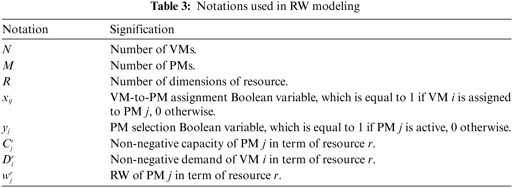
To quantify RW on multiple dimensions, we define the RW of PM j as the magnitude of wjr as Eq. (10). The total RW is defined in Eq. (11).

Wj=|wjr|(10)

W=∑j=1MWj(11)

3.1.5 Optimization Formulation

We aim to minimize EC, MC, and RW and maximize performance simultaneously. In the above model, we use the predicted values of VM resource demands (i.e., CPU demand prediction for EC, memory demand prediction for MC, and CPU and memory demand predictions for performance and RW) to calculate the objective function value.

Suppose fi(x) is the ith objective function entailed by a consolidation solution x. Let f1(x) be the function of EC described by [43], f2(x) be the function of performance defined by Eq. (2), f3(x) be the function of MC described by Eq. (8), and f4(x) be the function of RW described by Eq. (11). We can formulate VM consolidation problem as:

Minimize:[f1(x),f2(x),f3(x),f4(x)]

•   Constraint 1: ∑j=1Mxij=1. This means that one VM can be on only one PM.

•   Constraint 2: ∑i=1NDir⋅xij≤Cjryj. This guarantees that VM resource demands are not beyond PM capacity.

•   Constraint 3: yj,xij∈{0,1}.

3.2 The Suggested Prediction Approach

3.2.1 ARIMA Prediction Method

This paper uses the ARIMA model to map linear patterns in time series. ARIMA is a prediction and analysis model of time series. It can provide fast predictions [48]. It is very suitable for the prediction of the scaling of cloud resources. Through difference, it can transform the nonstationary time series into a stationary time series, and then apply AR and MA techniques to the time series. Reference [23] gives ARIMA model as follows:

yt=α0+β1yt−1+β2yt−2+⋯+βpyt−p+ϵt−α1ϵt−1−α2ϵt−2−⋯−αqϵt−q(12)

where βi(i=1,2,…,p) is AR coefficient at lag p,αi(i=0,1,…,q) is MA coefficient at lag q, and ϵt is the forecast error at period t, and yt is the actual value. The integers p and q are the orders of the model. In this paper, the Box-Jenkins method [49] fits ARIMA (p,d,q) model.

3.2.2 SVR Prediction Method

SVR is strong at extracting nonlinear patterns of time series. It optimally maps nonlinear input data to a higher-dimensional feature space through the transformation of the kernel function and then performs LR in feature space.

We give the original input training set as: {(x1,y1),(x2,y2),…,(xn,yn)}, where xi∈X⊂Rn,yi∈Y⊂R,i=1,2,…,n, n is a total number of samples. We need to find a separating hyperplane, such as f(x)=wTx+b=0, where w is normal vector, and b is a bias. We can write the distance from point x to hyperplane w,b as:

r=|wTx+b|||w||(13)

We write the margin width of the decision boundary as:

γ=2||w||(14)

We aim to minimize the number of samples that do not fulfill the constraint of decision boundary as much as possible. Thus, we write the optimization problem as:

minw,b12||w||2+C∑i=1nlϵ(f(xi)−yi)(15)

where C is regularization constant, lϵ is the loss function, and defined as:

lϵ(f(xi)−yi)={0|f(xi)−yi|≤ϵ|f(xi)−yi|−ϵotherwise(16)

To relax the samples’ margin requirements, slack variables ξi and ξi∗ are led into. We can display the optimization of SVR with slack variables below:

minw,b,ξi,ξi∗12||w||2+C∑i=1nξi+ξi∗(17)

s.t. f(xi)−yi≤ϵ+ξi,(18)

yi−f(xi)≤ϵ+ξi∗,

ξi≥0,ξi∗≥0,i=1,2,…,n.

Using Lagrange multipliers forms the dual optimization problem given by:

maxα,α^∑i=1nyi(αi^−αi)−ϵ(αi^+αi)−12∑i=1n∑j=1n(αi^−αi)(αj^−αj)xiTxj(19)

s.t.∑i=1n(αi^−αi)=0,(20)

0≤αi,αi^≤C,i=1,2,…,n.

f(x)=∑i=1n(αi^−αi)xiTx+b(21)

Let function φ(x) map n-dimensional vector x into m-dimensional vector x, where m > n. We can write f(x) as:

f(x)=∑i=1m(αi^−αi)φ(xi)Tφ(x)+b(22)

By using the kernel function, we can convert the calculation in the feature space into the calculation in the original space. The kernel function is defined as:

k(xi,xj)=<φ(xi),φ(xj)>=φ(xi)Tφ(xj)(23)

Therefore, we can overwrite f(x) as:

f(x)=∑i=1m(αi^−αi)k(x,xi)+b(24)

3.2.3 SMO

SMO is an algorithm usually used to solve optimization problems during the training process of SVM. This paper exploits it to solve the optimization problem in the training process of SVR. We describe the dual problem of SVR in Eq. (19). Let λi=αi^−αi, i=1,2,…,m, consider feature mapping and define kij=ϕ(xi)Tϕ(xj)=k(xi,xj), and we can express this problem as a minimization problem as below:

minλ∑i=1mϵ(|−λi|−(yiλi)+12∑i=1m∑j=1mλiλjkij(25)

s.t.∑i=1mλi=0,(26)

−C≤λi≤C, i=1,2,…,m.

If variables λ3,…,λm are regarded as constants, and then λ1+λ2=−∑i=3mλi=ς, assuming that variable λi≤0 (otherwise, the result remains the same), we can simplify the objective function as:

W(λ1,λ2)=12λ12k11+12λ12k22+λ1λ2k12+∑j=3mλ1λjk1j+∑j=3mλ2λjk2j−ϵ(λ1+λ2)−y1λ1−y2λ2(27)

On substituting λ1=ς−λ2 to Eq. (27), keep only the items with λ2, we can overwrite Eq. (27) as:

W(λ2)=12λ22k11−ςλ2k11+12λ22k22+ςλ2k12−λ22k12−∑j=3mλ2λjk1j+∑j=3mλ2λjk2j+y1λ2−y2λ2(28)

Find the partial derivative of function W concerning λ2 and let the derivative be zero as below:

∂W∂λ2=(k11+k22−2k12)λ2−(ςk11−ςk12+∑j=3mλjk1j−∑j=3mλjk2j+y2−y1)=0(29)

Let vi=∑j=3mλjkij=f(xi)−∑j=12λjkij−b,i=1,2,…,m, and substitute ς=λ1+λ2, there are:

(k11+k22−2k12)λ2=(k11+k22−2k12)λ2+E2−E1(30)

Ei=f(xi)−yi, i=1,2,…,m.(31)

Consequently, suppose that the solution of the last round is λ2old and the new solution of this round without clipping is λ2new,unc, we get:

λ2new,unc=λ2old+E2−E1k11+k22−2k12(32)

By clipping the original solution, we get:

λ2new{Hλ2new,unc>Hλ2new,uncL<λ2new,unc<HLλ2new,unc<L(33)

where L=λ1old+λ2old−C,H=C. Because of the linear relationship between variables λ1 and λ2, we can get:

λ1new=λ1old+λ2old−λ2new(34)

After optimizing the two variables, we need recalculate threshold b and error Ei. According to Karush-Kuhn-Tucker (KKT) conditions, when −C<λi<C, there are ξi=0 or ξi∗=0 and Eq. (35) holds:

{f(xi)−yi−ϵ=0−C<λi<0yi−f(xi)−ϵ=00<λi<C(35)

If −C<λ1new<0,

b=yi+ϵ−∑j=1mλjkij(36)

Therefore,

b1new=y1+ϵ−∑i=3mλiki1−λ1newk11−λ2newk21(37)

Due to:

E1=f(x1)−y1=∑i=3mλiki1+λ1oldk11+λ2oldk21+bold−y1(38)

We get:

b1new=−E1+ϵ+(λ1old−λ1new)k11+(λ2old−λ2new)k21+bold(39)

If −C<λ2new<0, we get:

b2new=−E2+ϵ+(λ1old−λ1new)k12+(λ2old−λ2new)k22+bold(40)

In the same way, if 0<λ1new<C and 0<λ2new<C, we get:

b1new=−E1−ϵ+(λ1old−λ1new)k11+(λ2old−λ2new)k21+bold(41)

b2new=−E2−ϵ+(λ1old−λ1new)k12+(λ2old−λ2new)k22+bold(42)

We take the new value of b as:

bnew=b1new+b2new2(43)

We can calculate Ei as:

Ei=∑i=1mλikij+bnew−yi(44)

The SMO process is repeated until all variables λi(i=1,2,…,m) are obtained.

4  Prediction-Based Multi-Objective VM Consolidation

4.1 Resource Usage Prediction

Dealing with dynamic resource requirements is necessary to minimize the total EC, MC, PD, and RW in a cloud data center. Knowing resource requirements in advance and buying time to calculate the optimization solution requires predicting future resource demand based on historical resource demand. This paper proposes a hybrid prediction approach based on ARIMA and SVR (HPAS) to predict VM resource demand using available resource demand history. We depict the framework of our prediction approach in Fig. 1. We utilize the resource demand trace generated from Microsoft Azure. We divide the resource demand data into two parts at a ratio of 6 to 4. For ARIMA, we train and test it to predict the future resource demand of VM. For SVR, we carry out the preprocessing phase. Then, we use the prepared and normalized resource demand data to train and test the SVR model. The SVR model predicts future errors. We depict the prediction model workflow in Fig. 2. We use an ARIMA model to predict the resource demand initially. As mentioned, the ARIMA model can only capture linear time series features. We use additional ARIMAs to calculate the errors but only consider linear attributes. History of residuals from multiple time slots (i.e., slots t−1,…,t−n+1) generated by ARIMAs is used to predict future error (i.e., slot t). Therefore, we use the residuals as inputs of the SVR model. Adding the forecasts of the ARIMA model (i.e., Xt) and the SVR model (i.e., Et^) obtains the final prediction (Ot^).

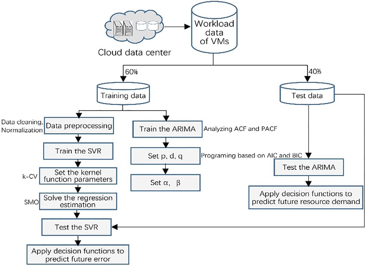
Figure 1: The prediction framework of resource demand

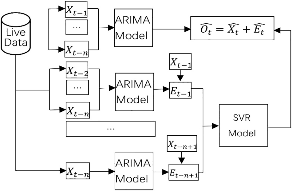
Figure 2: The prediction model workflow

From the above, we can see that in HPAS, ARIMA fully captures the linear features of live data from the past n time slots, but inevitably overlooks nonlinear features. We accumulate the error of using ARIMA only for prediction in the past n−1 time slots through n−1 additional ARIMAs. These errors contain sufficient nonlinear features of live data and serve as inputs for SVR. Therefore, SVR can fully capture the nonlinear features of live data from the past n−1 time slots. SVR predicts the nonlinear part of VM resource demand in time slot t and finally revises the initial ARIMA prediction of VM resource demand for time slot t. Consequently, HPAS results in better predictive performance than only one of ARIMA and SVR.

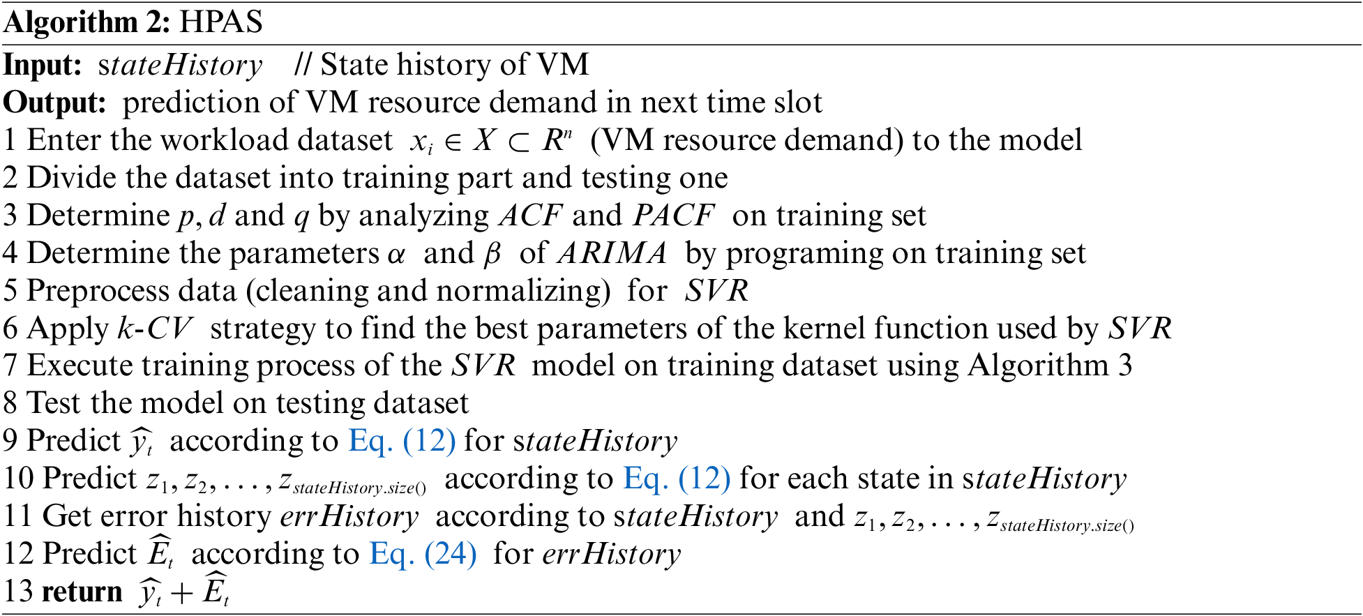
We present the pseudo-code for predicting resource demand per VM in Algorithm 2. Initially, we enter the dataset into the suggested model (line 1). We partition the dataset into two parts: the training part and the testing one (line 2). The training part estimates the ARIMA model by analyzing AC and partial PAC functions and programming (lines 3–4). Next, we preprocess the generated resource demand data for SVR (line 5). We use the boxplot method to detect outliers, remove them, and use interpolation to fill in missing values to implement regression smoothly. We then apply the K-fold Cross Validation (k-CV) strategy to select the best parameters of the kernel function (i.e., γ, C, and ε) used by SVR (line 6). We perform the training process with the normalized resource demand data and the suitable parameters (line 7). In the testing phase, the test evaluates the suggested model’s prediction accuracy (line 8). Finally, we obtained the prediction result (lines 9–13).

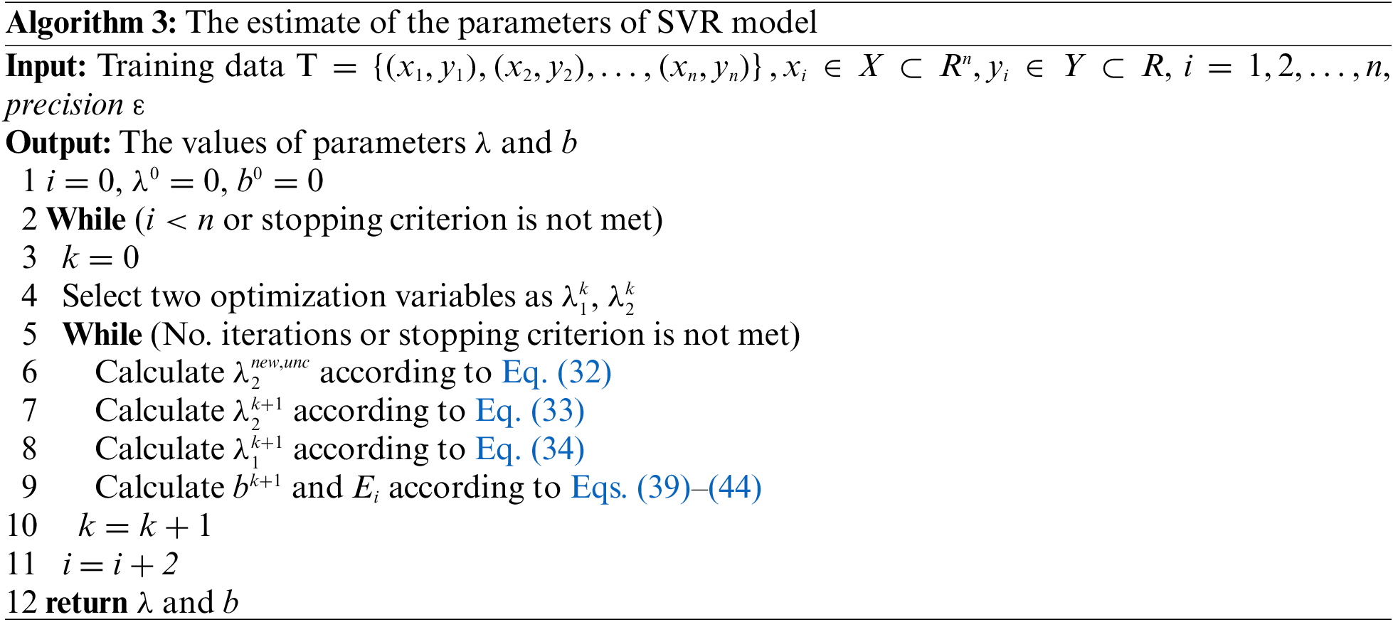
We performed the training process to get the best parameters of the SVR model using Algorithm 3. The first line is initialization. We then pick two variables (line 4). The first variable λ1k selects the sample with the most severe violation of KKT conditions in the training set. If all samples meet the KKT condition, select a sample randomly. After selecting λ1k, the second variable λ2k selects the sample with enough change for |E1−E2|. Next, we optimize λ1k and λ2k repeatedly using Eqs. (32)–(34), (39)–(44) until we reach maximum iteration or satisfy the termination condition (lines 5–10). Finally, we complete the optimization of all the variables λi(i=1,…,n) and b.

4.2 VM Consolidation

The main goal of this work is to consolidate VMs into PMs based on the prediction result. We propose an efficient prediction-based multi-objective VM consolidation algorithm that aims to minimize the total EC, PD, MC, and RW in a cloud data center, depending on future resource demand.

4.2.1 Overload/Underload PM Detection

Algorithm 4 represents the overload/underload PM detection procedure. We used a warm-up window to ensure computational tractability [44]. This paper’s first warmUpWindowSize time slots were regarded as a warm-up phase (line 5). During the warm-up phase, we calculate the CPU usage of PM and choose overload/underload PM (lines 1–6, lines 11–12). After the warm-up phase, we use the prediction result of Algorithm 2 to calculate the CPU usage of PM and choose over/lower utilized PMs (line 8).

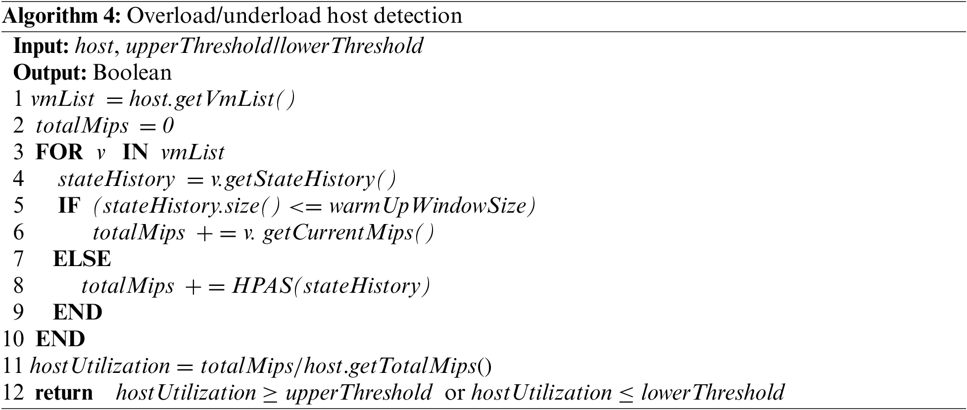
All the VMs of underload hosts need to migrate, and we shut all the underload hosts down to save EC and decrease RW.

4.2.2 VM Selection

We chose the MMT policy for VM selection. MMT policy selects a VM that requires the minimum time to complete a migration. The migration time is the amount of RAM the VM utilizes divided by the spare network bandwidth available for the PM.

4.2.3 VM Placement

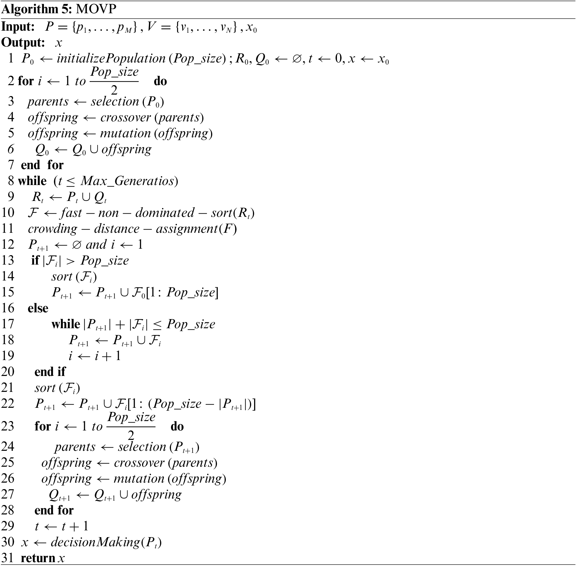
We perform multi-objective optimization VM placement to reduce EC, PD, MC, and RW simultaneously. We develop a multi-objective optimization VM placement (MOVP) approach based on the Nsga2 algorithm.

Pareto dominance is widely used in the search for a multi-objective optimization solution. Consider two solutions u,v∈X, u dominate v, denoted as u>v, if and only if f(u) is superior to or equal to f(v) in each objective function and strictly superior in at least one objective function. It is called solution x is non-dominant for set X, if there is no dominant member in X. The solution of multi-objective optimization is called the Pareto optimal set. No other solution dominates the solutions in the Pareto optimal set. The corresponding set of objective values defines the Pareto frontier.

Each placement solution is a vector x as described in Section 3.1.5. In MOVP, the objective functions are defined in Sections 3.1.1–3.1.4, as described in Section 3.1.5. It is worth noting that when calculating the values of these objective functions, we use the resource demand values (i.e., CPU utilization and Memory usage) of the VM predicted through HPVS. Using the predicted value of resource demands instead of the current value for MOVP can give the placement solution good timeliness and practical value. We present the pseudo-code for VM placement in Algorithm 5, which inputs the PM, VM sets, and initial placement solution x0. Initially, we built a random parent population P0 (line 1). We use selection, crossover, and mutation operators to create an offspring population Q0 of size Pop_size (lines 3–5). In each generation, a merged population Rt of size 2⋅Pop_size is formed to prevent individuals from being lost in the next generation in line 7. Next, we sort the population Rt in non-domination order and arrange individuals into different frontiers (line 9). Function crowding−distance−assignment is used to ensure the diversity of individuals (line 10). We choose individuals from several frontiers (frontier order from low to high, i.e., ℱ1,ℱ2, and so on) for new population Pt+1. To determine exactly Pop_size individuals, we sort the individuals of the last frontier ℱi using the crowd-comparison operator in descending order (lines 14, 21) and select enough individuals (lines 15–22). Then, we generate offspring Qt+1 of Pt+1 for the next iteration (lines 23–28). Function decisionMaking is an operator that chooses favorite individuals from current Pareto optimal set Pt (line 30).

Fast−non−dominated−sort and crowding−distance−assignment are the two fundamental operations of Nsga2, which will not be further elaborated here to save space.

5  Evaluation

This section evaluates the proposed approach based on the results obtained. First, the prediction accuracy of the suggested prediction model is evaluated, and then the prediction-based consolidation of the proposed approach is evaluated.

5.1 Experimental Setup

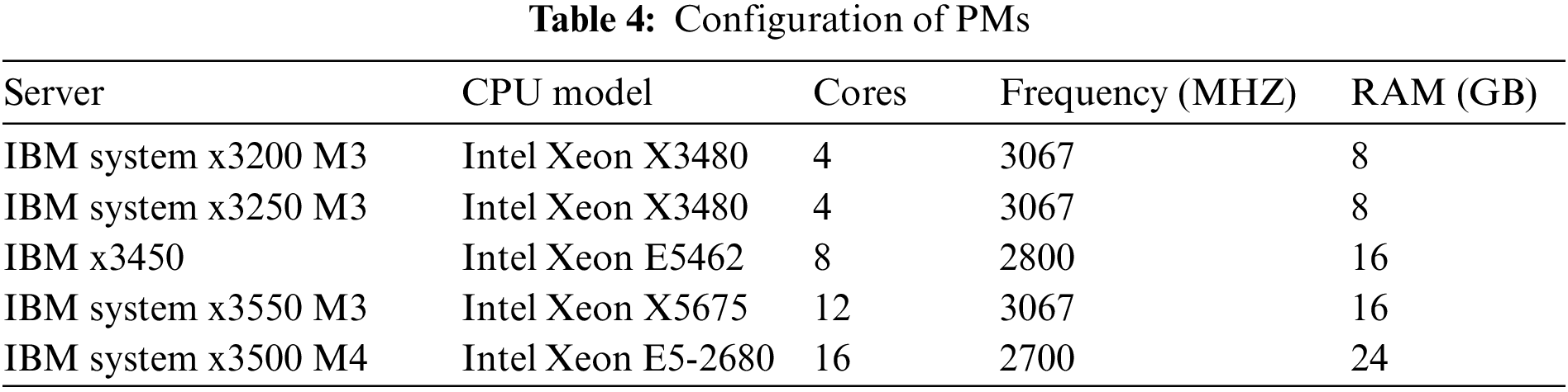
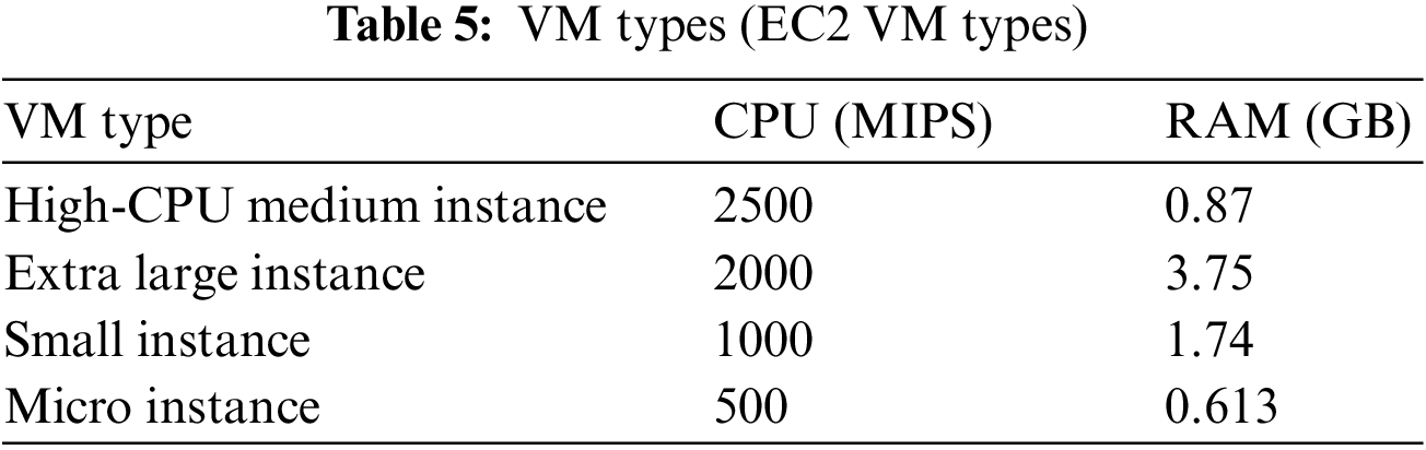
We performed a simulation on CloudSim version 5.0. We simulated a cloud data center with 50 heterogeneous PMs in five configurations. Table 4 describes the characteristics of these machines. VMs are supposed to correspond to Amazon EC2 instance types. The experiments use four types of VMs, as shown in Table 5. After each VM consolidation step, VM resource demand changes according to workload data.

We use the parameters of HPAS, C, ε, and γ to adjust the tradeoff between model complexity and training error, define the accuracy requirement, and facilitate the mapping of input data, respectively [19]. We obtain a better performance of HPAS when C is 150, ε is 0.01, and γ is 0.0001.

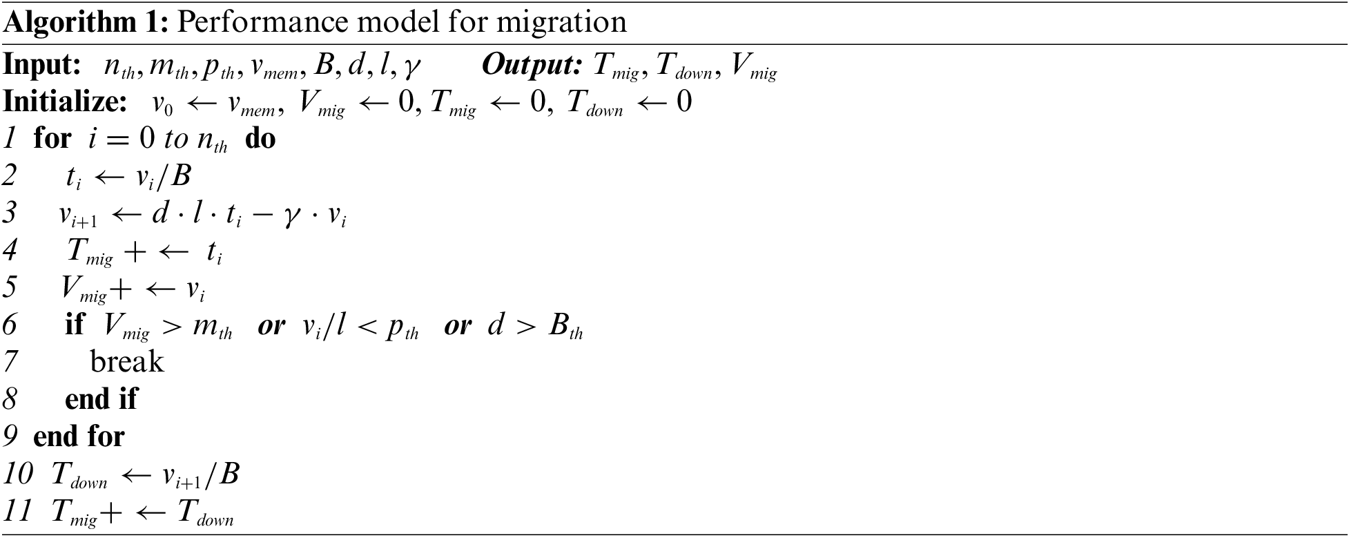
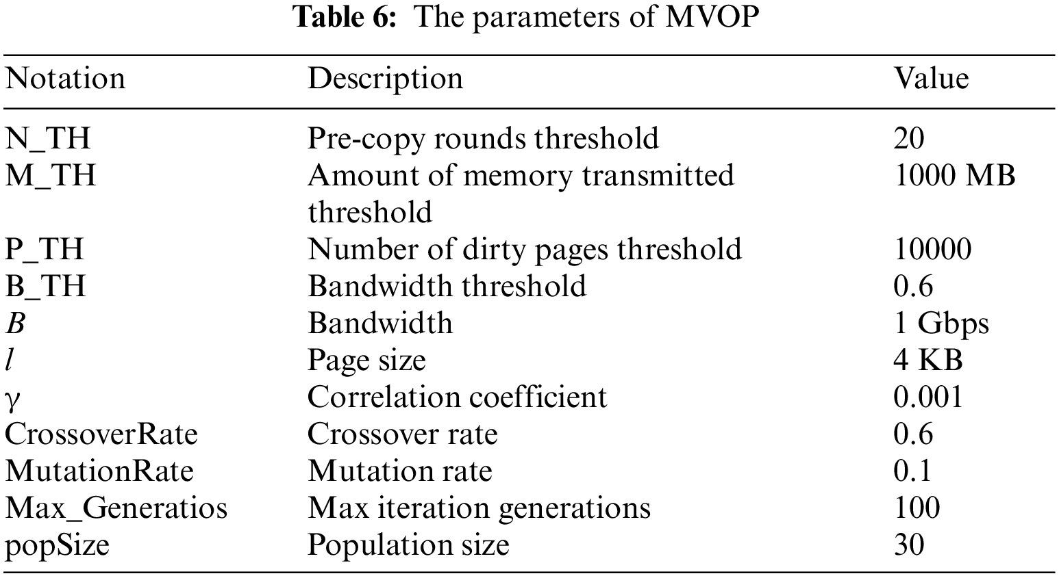
Table 6 presents MOVP’s parameters. The first seven are used by Algorithm 1, which MOVP invokes.

We performed each experiment 10 times for our proposed approach, and reported the mean values for different metrics.

5.2 Workload Model

It is essential to conduct experiments using workload traces from a real system. We used MicroSoft Azure trace as resource demand data. This data trace contains information about every VM running on Azure from 16 November 2016, to 16 February 2017. The data-trace corresponds to tens of millions of VMs from tens of thousands of first- and third-party users.

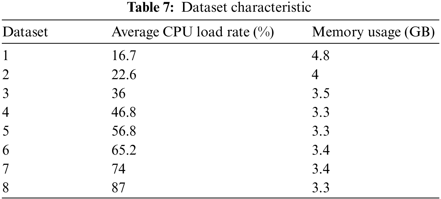
In Sections 5.3 and 5.4, we conducted comparative experiments between the proposed and benchmark algorithms using diverse datasets obtained from Azure Trace. These datasets’ average CPU load rates are low to high, and their memories are relatively stable. We give the characteristics of all the datasets in Table 7.

5.3 Evaluation of Prediction Accuracy

5.3.1 Evaluation Metrics

We use several metrics to evaluate prediction accuracy for the suggested prediction model. The evaluation metrics include Root Mean Square Error (RMSE), Mean Absolute Percentage (MAPE), Mean Absolute Error (MAE), and R-squared (R2) [50].

5.3.2 Results

We compare HPAS’ forecast accuracy with state-of-the-art approaches to its efficacy. ARIMA and SVR are two promising prediction methods for linear and nonlinear loads, respectively. The back propagation neural network (BP-NN) is one of the most widely used neural network models. Thus, we adopt them as baseline approaches.

We used 400 VMs and adopted Microsoft Azure data trace as the VM’s resource demand. Table 8 shows the comparison in terms of evaluation metrics in four hours. The table indicates that ARIMA performs worst, followed by SVR and BP-NN. HPAS performs best. The low value of RMSE indicates high accuracy. The value of RMSE for HPAS is the lowest. In terms of MAPE and MAE, HPAS performs the best. As we all know, the value of R2 close to 1 indicates a good fit of data. HPAS is closer to 1 than existing approaches.

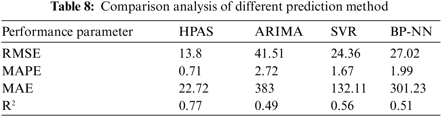
In summary, HPAS shows better prediction accuracy, followed by SVR, BP-NN, and ARIMA. HPAS’ better prediction accuracy can be explained by the proposed approach’s powerful capacity to capture linear and nonlinear data features simultaneously.

Table 9 compares diverse kernel functions used in HPAS. We want to see whether HPAS uses RBF kernel functions, which can produce better RMSE, MAPE, MAE, and R2 results, compared to Linear, Polynomial, and Sigmoid kernel functions. If R2 is negative (i.e., Linear and Sigmoid), it indicates that the fitting result is unreliable because the two kernel functions do not match data.

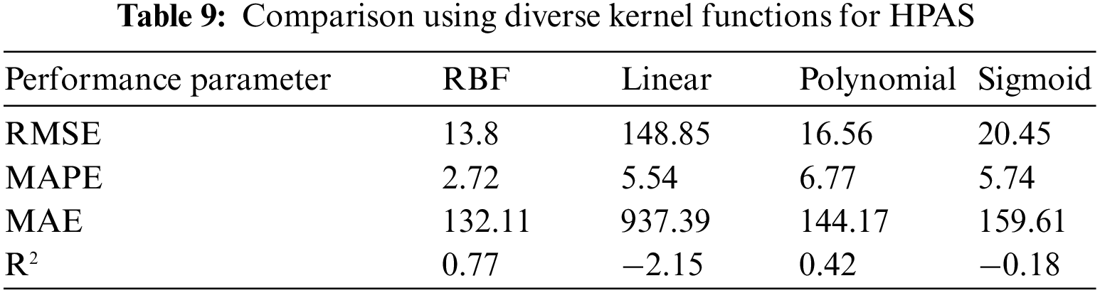
Fig. 3 provides prediction using different prediction methods. For ARIMA and SVR, the prediction is accurate for a few time slot points and cannot reflect the trend of changes in actual values, as shown in Fig. 3a,b. For BP-NN, The predicted value is generally smaller than the actual value and cannot reflect the trend of changes in actual values either, as shown in Fig. 3c. HPAS gives better prediction results, as shown in Fig. 3d. In the initial stage (the time slot before point 55), the relationship between actual and predicted values is quite chaotic due to the small number of samples in the prediction set. Afterward, as the number of samples in the prediction set increases, the predicted values reflect the trend of changes in actual values at many points, such as the sharp shapes near time slot points 57, 61, 63, 71, 101, and 121. At some points, the predicted value almost coincides with the actual value, such as time slot points 58, 63, 67, 69, 80, 86, 88, 99, 107, 112, 118, and 124.

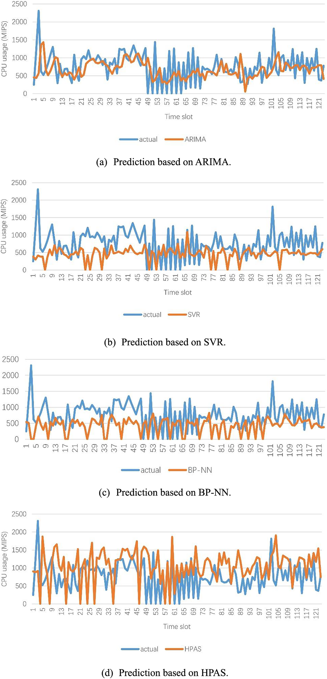
Figure 3: Comparison of actual and predicted values using different prediction method (a–d)

We can conclude that HPAS’ predictions will become more accurate as the prediction sample set grows. The results convey that HPAS produces more accurate forecasts than other prediction methods.

5.4 Evaluation of VM Consolidation

5.4.1 Evaluation Metrics

We evaluate our approach using metrics corresponding to the objectives proposed in Section 4, such as EC, SLA violation, MC, and RW. We also use the number of VM migrations and computation time as additional metrics.

5.4.2 Results

We first compare our approach with the multi-objective VM consolidation approach without prediction. We chose the VM consolidation approach adopting the Nsga2 algorithm for multi-objective optimization as a baseline approach.

Fig. 4 illustrates the metrics produced by the two approaches for six different datasets in four hours. Our consolidation approach consumed less power than Nsga2 except for datasets 4 and 6. EC was reduced by 3.1% in the worst case and by 37.7% in the best case compared to Nsga2. SLAV was significantly reduced for all the datasets. It was reduced by 11.3% in the worst case and by 88.5% in the best case compared to Nsga2. MC was reduced by 4% in the worst case and by 48.7% in the best case compared to Nsga2. The number of VM migrations was significantly reduced for all the datasets. It was reduced by 24.5% in the worst case and by 68.7% in the best case compared to Nsga2. There was a slight reduction in RW. In terms of computation time, our approach spent more time than Nsga2. It was increased by 431% in the worst case and 3% in the best case compared to Nsga2, which can be explained by the fact that our approach integrates two prediction models (i.e., ARIMA and SVR), and their training and prediction processes are time-consuming tasks, especially SVR. Another reason is that calling the ARIMA model multiple times to obtain error history data takes some time.

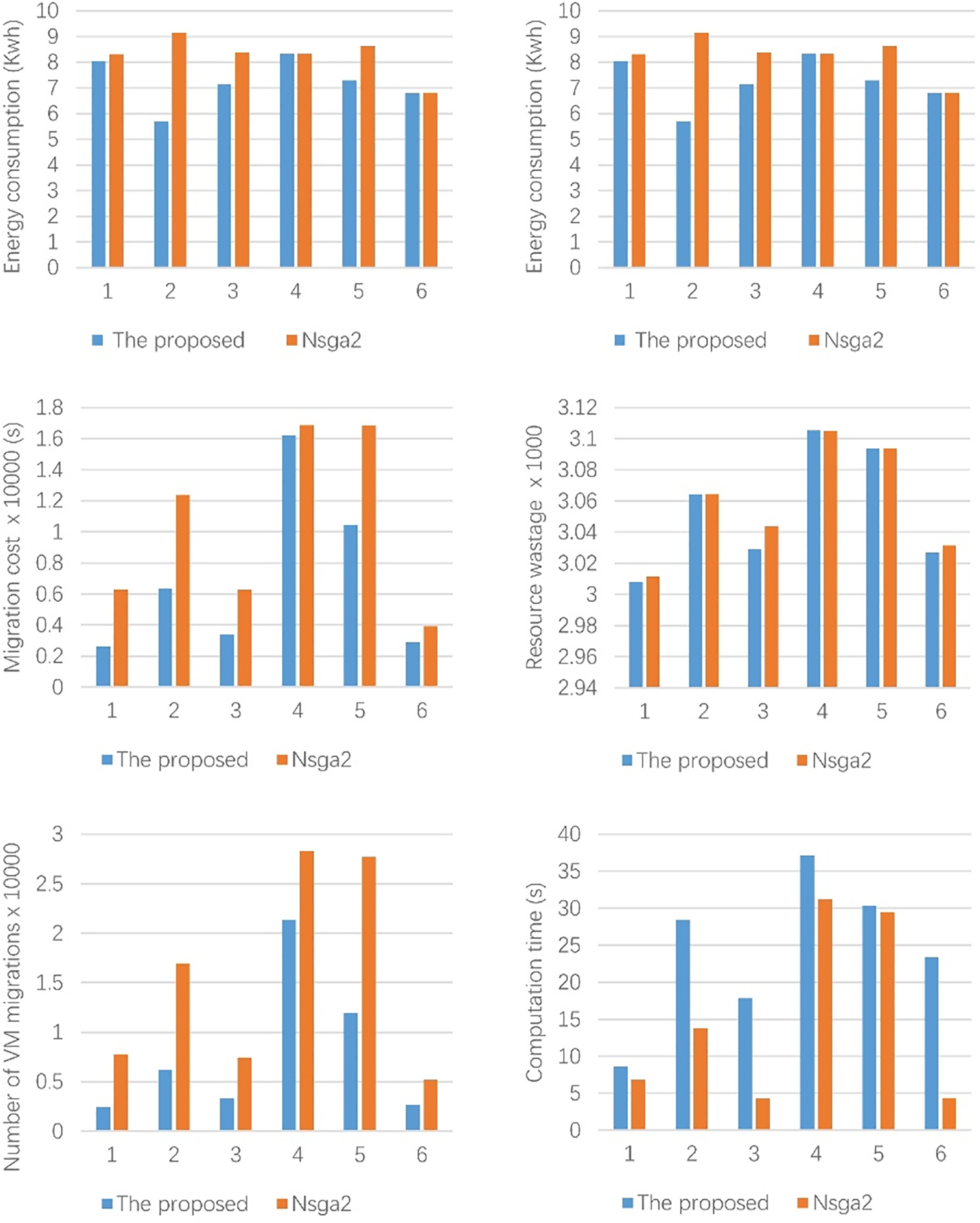
Figure 4: Comparison between the proposed approach and Nsga2 with different dataset

In summary, the proposed approach has an excellent performance in terms of EC, SLAV, MC, and number of VM migrations, which is attributed to the high predictive capacity of our approach. Our approach provides the foresight of overload and underload detection, avoiding the issue of detection results becoming invalid soon after, which also provides the foresight of VM selection, avoiding the issue of selecting too many or too few VMs, and the foresight of destination PM selection, avoiding the issue of target PM accommodating too many or too few VMs.

Next, we compare our approach with the renowned OHD approaches without prediction, such as LR, MAD, and IQR. LR predicts CPU utilizations using LR. MAD and IQR measure the workload stability by calculating the median absolute deviation and interquartile range of CPU utilization. Fig. 5 illustrates the metrics produced by all the approaches for six different datasets in two hours.

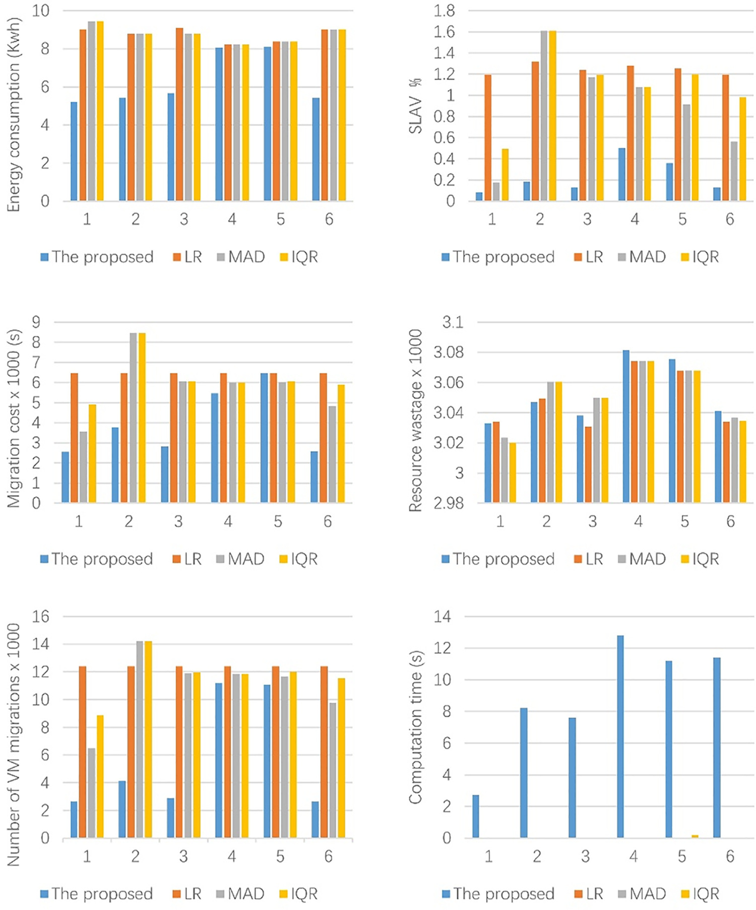
Figure 5: Comparison between the proposed approach and the existing OHD algorithms with different dataset

As shown in Fig. 5, our approach consumed less energy than any of the three approaches. Compared to the best of the three algorithms (i.e., LR), EC was reduced by 3.1% in the worst case and by 42.2% in the best case. SLAV was significantly reduced for all the datasets. Compared to the best of the three algorithms (i.e., MAD), SLAV was reduced by 52.2% in the worst case and by 88.8% in the best case. MC was greatly reduced except for dataset 5. Compared to the best of the three algorithms (i.e., MAD), it was reduced by 8% in the worst case and by 55.3% in the best case. The number of VM migrations was significantly reduced for all the datasets. Compared to the best of the three algorithms (i.e., MAD), it was reduced by 4.9% in the worst case and by 75.9% in the best case. The excellent performance of our approach can be explained by the fact that MAD and IQR provide adaptive utilization thresholds based on statistics and cannot learn, LR has weak predictive ability for nonlinear data, and our approach can better predict future resource demand for both linear and nonlinear data, enabling overload and underload detection more accurate.

There is not much improvement in RW. Regarding computation time, our approach spent more time than the three approaches. This is explained by the fact that LR, MAD, and IQR only require simple calculations compared to our approach.

6  Conclusion and Future Work

In this paper, we have proposed a prediction-based multi-objective VM consolidation approach, which predicts future VM resource demand using HPAS, then consolidates VMs to PMs based on prediction results by HPAS, aiming at simultaneously minimizing the total EC, PD, MC, and RW. We have evaluated the proposed approach through simulation using real workload traces from Microsoft Azure. The results illustrate that the proposed prediction model shows better prediction accuracy, and the proposed consolidation approach overcomes the multi-objective consolidation approach without prediction and the renowned OHD approaches without prediction, such as LR, MAD, and IQR.

Our approach powerfully captures both linear and nonlinear features of data, enabling timely overload and underload detection, accurate VM and destination PM selections, and avoiding of unnecessary VM migrations.

As this work is the first step in developing the best VM consolidation approach, we only evaluated our approach in a simulation environment. In the future, we plan to study the effect of the proposed approach in a real cloud environment. In two hours, the time spent on training, predicting, and multi-objective optimization 2–13 s. The time cost is reasonable for small and medium-sized cloud data centers. However, combining grouping technology based on this work is more suitable for large-sized cloud data centers.

Acknowledgement: We sincerely appreciate Xinfeng Shu’s valuable guidance and suggestions in this study. At the same time, we also appreciate the experimental equipment provided by Shaanxi Key Laboratory of Network Data Analysis and Intelligent Processing. In addition, we would like to thank all colleagues and collaborators who participated in this study for their hard work and selfless dedication, which enabled the successful completion of this study.

Funding Statement: This study was funded by Science and Technology Department of Shaanxi Province, Grant Numbers: 2019GY-020 and 2024JC-YBQN-0730. This organization did not influence the study design, data collection, analysis, interpretation, manuscript writing, or the decision to submit the manuscript for publication.

Author Contributions: Conceptualization: Xialin Liu; Methodology: Xialin Liu; Software: Xialin Liu; Validation: Jiyuan Hu; Formal Analysis: Xialin Liu; Investigation: All authors; Resources: Junsheng Wu; Data Curation: Lijun Chen; Writing–Original Draft: Xialin Liu; Writing–Review & Editing: All authors; Visualization: Lijun Chen; Funding Acquisition: Junsheng Wu. All authors reviewed the results and approved the final version of the manuscript.

Availability of Data and Materials: All data and materials included in this study are available upon request by contacting the corresponding author.

Conflicts of Interest: We declare that we have no financial and personal relationships with other people or organizations that can inappropriately influence our work, and there is no professional or other personal interest of any nature or kind in any product, service, or company that could be construed as influencing the position presented in, or the review of, the manuscript entitled “A Prediction-Based Multi-Objective VM Consolidation Approach for Cloud Data Centers”.

References

1. M. Tavana, S. Shahdi-Pashaki, E. Teymourian, F. J. Santos-Arteaga, and M. Komaki, “A discrete cuckoo optimization algorithm for consolidation in cloud computing,” Comput. Ind. Eng., vol. 115, no. 1, pp. 495–511, Jan. 2018. doi: 10.1016/j.cie.2017.12.001. [Google Scholar] [CrossRef]

2. D. Saxena and A. K. Singh, “A proactive autoscaling and energy-efficient VM allocation framework using online multi-resource neural network for cloud data center,” Neurocomputing, vol. 426, no. 6, pp. 248–264, Feb. 2021. doi: 10.1016/j.neucom.2020.08.076. [Google Scholar] [CrossRef]

3. S. Mashhadi Moghaddam, M. O’Sullivan, C. Walker, S. Fotuhi Piraghaj, and C. P. Unsworth, “Embedding individualized machine learning prediction models for energy efficient VM consolidation within Cloud data centers,” Future Gener. Comput. Syst., vol. 106, no. 1, pp. 221–233, Jan. 2020. doi: 10.1016/j.future.2020.01.008. [Google Scholar] [CrossRef]

4. N. K. Biswas, S. Banerjee, U. Biswas, and U. Ghosh, “An approach towards development of new linear regression prediction model for reduced energy consumption and SLA violation in the domain of green cloud computing,” Sustain. Energy Technol., vol. 45, no. 4, pp. 101087, Jun. 2021. doi: 10.1016/j.seta.2021.101087. [Google Scholar] [CrossRef]

5. T. C. Ferreto, M. A. S. Netto, R. N. Calheiros, and C. A. F. de Rose, “Server consolidation with migration control for virtualized data centers,” Future Gener. Comput. Syst., vol. 27, no. 8, pp. 1027–1034, Oct. 2011. doi: 10.1016/j.future.2011.04.016. [Google Scholar] [CrossRef]

6. I. Takouna, E. Alzaghoul, and C. Meinel, “Robust virtual machine consolidation for efficient energy and performance in virtualized data centers,” presented at the 2014 IEEE Int. Conf. Green. Comput., Taipei, Taiwan, Sep. 1–3, 2014. [Google Scholar]

7. J. Jheng, F. Tseng, H. Chao, and L. D. Chou, “A novel VM workload prediction using grey forecasting model in cloud data center,” presented at the 2014 Int. Conf. Inf. Net., Phuket, Thailand, Feb. 10–12, 2014. [Google Scholar]

8. S. Y. Hsieh, C. S. Liu, R. Buyya, and A. Y. Zomaya, “Utilization-prediction-aware virtual machine consolidation approach for energy-efficient cloud data centers,” J. Parallel. Distr. Comput., vol. 139, pp. 99–109, May 2020. doi: 10.1016/j.jpdc.2019.12.014. [Google Scholar] [CrossRef]

9. M. H. Sayadnavard, A. Toroghi Haghighat, and A. M. Rahmani, “A multi-objective approach for energy-efficientand reliable dynamic VM consolidation in cloud data centers,” Eng. Sci. Technol., vol. 26, no. 2, pp. 100995, Feb. 2021. doi: 10.1016/j.jestch.2021.04.014. [Google Scholar] [CrossRef]

10. L. Li, J. Dong, D. Zuo, and J. Liu, “SLA-aware and energy-efficient VM consolidation in cloud data centers using host states naive bayesian prediction model,” presented at the 2018 IEEE. Int. Conf. Ubiq. Comput., Melbourne, VC, AUS, Dec. 11–13, 2018. [Google Scholar]

11. R. N. Calheiros, E. Masoumi, R. Ranjan, and R. Buyya, “Workload prediction using ARIMA model and its impact on cloud applications’ QoS,” IEEE Trans. Cloud Comput., vol. 3, no. 4, pp. 449–458, Aug. 2015. doi: 10.1109/TCC.2014.2350475. [Google Scholar] [CrossRef]

12. F. Farahnakian, P. Liljeberg, and J. Plosila, “LiRCUP: Linear regression based CPU usage prediction algorithm for live migration of virtual machines in data centers,” presented at the 2013 Euro. Conf. Soft. Eng. Adv. Appl., Santander, Spain, Sep. 4–6, 2013. [Google Scholar]

13. F. Farahnakian et al., “Using ant colony system to consolidate VMS for green cloud computing,” IEEE Trans. Serv. Comput., vol. 2, pp. 187–198, Oct. 2015. doi: 10.1109/TSC.2014.2382555. [Google Scholar] [CrossRef]

14. N. T. Hieu, M. D. Francesco, and A. Ylä-Jääski, “Virtual machine consolidation with usage prediction for energy-efficient cloud data centers,” presented at the 2015 IEEE 8th Int. Conf. Clou. Comput., New York, USA, Jun. 27–Jul. 2, 2015. [Google Scholar]

15. S. B. Shaw, J. P. Kumar, and A. K. Singh, “Energy-performance trade-off through restricted virtual machine consolidation in cloud data center,” presented at the 2017 Int. Conf. Inte. Comput. Cont., Coimbatore, India, Jun. 23–24, 2017. [Google Scholar]

16. F. Farahnakian, T. Pahikkala, P. Liljeberg, and J. Plosila, “Energy aware consolidation algorithm based on k-nearest neighbor regression for cloud data centers,” presented at the 2013 IEEE/ACM Int. Conf. Util. Clou. Comput., Dresden, Germany, Dec. 9–12, 2013. [Google Scholar]

17. Z. Li, C. Yan, X. Yu, and N. Yu, “Bayesian network-based virtual machines consolidation method,” Future Gener. Comput. Syst., vol. 69, no. 7, pp. 75–87, Apr. 2017. doi: 10.1016/j.future.2016.12.008. [Google Scholar] [CrossRef]

18. J. Kumar, A. K. Singh, and R. Buyya, “Self directed learning based workload forecasting model for cloud resource management,” Inform. Sci., vol. 543, no. 1, pp. 345–366, Jan. 2021. doi: 10.1016/j.ins.2020.07.012. [Google Scholar] [CrossRef]

19. L. Abdullah, H. Li, S. Al-Jamali, A. Al-Badwi, and C. Ruan, “Predicting multi-attribute host resource utilization using support vector regression technique,” IEEE Access, vol. 8, pp. 66048–66067, Mar. 2020. doi: 10.1109/ACCESS.2020.2984056. [Google Scholar] [CrossRef]

20. T. Thein, M. M. Myo, S. Parvin, and A. Gawanmeh, “Reinforcement learning based methodology for energy-efficient resource allocation in cloud data centers,” J. King Saud Univ-Comput., vol. 32, no. 10, pp. 1127–1139, Dec. 2020. doi: 10.1016/j.jksuci.2018.11.005. [Google Scholar] [CrossRef]

21. M. Ghobaei-Arani, S. Jabbehdari, and M. A. Pourmina, “An autonomic resource provisioning approach for service-based cloud applications: A hybrid approach,” Future Gener. Comput. Syst., vol. 78, no. 3, pp. 191–210, Jan. 2018. doi: 10.1016/j.future.2017.02.022. [Google Scholar] [CrossRef]

22. Y. Liu, X. Sun, W. Wei, and W. Jing, “Enhancing energy-efficient and QoS dynamic virtual machine consolidation method in cloud environment,” IEEE Access, vol. 6, pp. 31224–31235, May 2018. doi: 10.1109/ACCESS.2018.2835670. [Google Scholar] [CrossRef]

23. H. A. Kholidy, “An intelligent swarm based prediction approach for predicting cloud computing user resource needs,” Comput. Commun., vol. 151, no. 1, pp. 133–144, Feb. 2020. doi: 10.1016/j.comcom.2019.12.028. [Google Scholar] [CrossRef]

24. Z. U. Qazi, H. Shahzad, and K. G. Muhammad, “Adaptive resource utilization prediction system for infrastructure as a service cloud,” Comput. Intell. Neurosci., vol. 2017, pp. 4873459, Jul. 2017. doi: 10.1155/2017/4873459. [Google Scholar] [PubMed] [CrossRef]

25. J. Kumar, A. K. Singh, and R. Buyya, “Ensemble learning based predictive framework for virtual machine resource request prediction,” Neurocomputing, vol. 397, no. 5, pp. 20–30, Jul. 2020. doi: 10.1016/j.neucom.2020.02.014. [Google Scholar] [CrossRef]

26. G. Kaur, A. Bala, and I. Chana, “An intelligent regressive ensemble approach for predicting resource usage in cloud computing,” J. Parallel. Distr. Comput., vol. 123, no. 1, pp. 1–12, Jan. 2019. doi: 10.1016/j.jpdc.2018.08.008. [Google Scholar] [CrossRef]

27. J. Subirats and J. Guitart, “Assessing and forecasting energy efficiency on cloud computing platforms,” Future Gener. Comput. Syst., vol. 45, no. 1, pp. 70–94, Apr. 2015. doi: 10.1016/j.future.2014.11.008. [Google Scholar] [CrossRef]

28. K. Mason, M. Duggan, E. Barrett, J. Duggan, and E. Howley, “Predicting host CPU utilization in the cloud using evolutionary neural networks,” Future Gener. Comput. Syst., vol. 86, no. 4, pp. 162–173, Sep. 2018. doi: 10.1016/j.future.2018.03.040. [Google Scholar] [CrossRef]

29. J. Kumar, R. Goomer, and A. K. Singh, “Long short term memory recurrent neural network (LSTM-RNN) based workload forecasting model for cloud datacenters,” Procedia Comput., vol. 125, no. 3, pp. 676–682, 2018. doi: 10.1016/j.procs.2017.12.087. [Google Scholar] [CrossRef]

30. Y. Zhang, J. Yao, and H. Guan, “Intelligent cloud resource management with deep reinforcement learning,” IEEE Cloud Comput., vol. 4, no. 6, pp. 60–69, Dec. 2017. doi: 10.1109/MCC.2018.1081063. [Google Scholar] [CrossRef]

31. B. Hariharan, R. Siva, S. Kaliraj, and P. N. Senthil Prakash, “ABSO: An energy-efficient multi-objective VM consolidation using adaptive beetle swarm optimization on cloud environment,” J. Amb. Intell. Hum. Comput., vol. 14, no. 3, pp. 2185–2197, Aug. 2021. doi: 10.1007/s12652-021-03429-w. [Google Scholar] [CrossRef]

32. M. Sharifi, H. Salimi, and M. Najafzadeh, “Power-efficient distributed scheduling of virtual machines using workload-aware consolidation techniques,” J. Supercomput., vol. 61, no. 1, pp. 46–66, Jul. 2011. doi: 10.1007/s11227-011-0658-5. [Google Scholar] [CrossRef]

33. M. Ghetas, “A multi-objective monarch butterfly algorithm for virtual machine placement in cloud computing,” Neur. Comput. Appl., vol. 33, no. 17, pp. 11011–11025, Jan. 2021. doi: 10.1007/s00521-020-05559-2. [Google Scholar] [CrossRef]

34. S. Mazumdar and M. Pranzo, “Power efficient server consolidation for cloud data center,” Future Gener. Comput. Syst., vol. 70, pp. 4–16, May 2017. doi: 10.1016/j.future.2016.12.022. [Google Scholar] [CrossRef]

35. M. A. Elshabka, H. A. Hassan, W. M. Sheta, and H. M. Harb, “Security-aware dynamic VM consolidation,” Egypt. Inform. J., vol. 13, pp. 277–284, Sep. 2020. doi: 10.1016/j.eij.2020.10.00. [Google Scholar] [CrossRef]

36. Y. Sharma, W. Si, D. Sun, and B. Javadi, “Failure-aware energy-efficient VM consolidation in cloud computing systems,” Future Gener. Comput. Syst., vol. 94, pp. 620–633, May 2019. doi: 10.1016/j.future.2018.11.052. [Google Scholar] [CrossRef]

37. B. M. P. Moura, G. B. Schneider, A. C. Yamin, H. Santos, R. H. S. Reiser and B. Bedregal, “Interval-valued fuzzy logic approach for overloaded hosts in consolidation of virtual machines in cloud computing,” Fuzz. Sets Syst., vol. 446, no. 4, pp. 144–166, Oct. 2022. doi: 10.1016/j.fss.2021.03.001. [Google Scholar] [CrossRef]

38. N. Kord and H. Haghighi, “An energy-efficient approach for virtual machine placement in cloud based data centers,” presented at the 2013 5th Conf. Info. Know. Tech., Shiraz, Iran, May 28–30, 2013. [Google Scholar]

39. Q. Liao and Z. Wang, “Energy consumption optimization scheme of cloud data center based on SDN,” Procedia Comput. Sci., vol. 131, no. 5, pp. 1318–1327, Jan. 2018. doi: 10.1016/j.procs.2018.04.327. [Google Scholar] [CrossRef]

40. S. Gharehpasha and M. Masdari, “A discrete chaotic multi-objective SCA-ALO optimization algorithm for an optimal virtual machine placement in cloud data center,” J Amb. Intell. Hum. Comp., vol. 12, Nov. 2020. doi: 10.1007/s12652-020-02645-0. [Google Scholar] [CrossRef]

41. Y. Gao, H. Guan, Z. Qi, Y. Hou, and L. Liu, “A multi-objective ant colony system algorithm for virtual machine placement in cloud computing,” J. Comput. Syst Sci., vol. 79, no. 8, pp. 1230–1242, Dec. 2013. doi: 10.1016/j.jcss.2013.02.004. [Google Scholar] [CrossRef]

42. M. H. Malekloo, N. Kara, and M. E. Barachi, “An energy efficient and SLA compliant approach for resource allocation and consolidation in cloud computing environments,” Sustain. Comput-Infor., vol. 17, pp. 9–24, Mar. 2018. doi: 10.1016/j.suscom.2018.02.001. [Google Scholar] [CrossRef]

43. X. Liu, J. Wu, L. Chen, and L. Zhang, “Energy-aware virtual machine consolidation based on evolutionary game theory,” Concurr. Comp-Pract. E, vol. 34, no. 10, pp. e6830.1–e6830.16, May 2022. doi: 10.1002/cpe.6830. [Google Scholar] [CrossRef]

44. A. Beloglazov and R. Buyya, “Optimal online deterministic algorithms and adaptive heuristics for energy and performance efficient dynamic consolidation of virtual machines in cloud data centers,” Concurr. Comp-Pract. E, vol. 24, no. 13, pp. 1397–1420, Oct. 2011. doi: 10.1002/cpe.1867. [Google Scholar] [CrossRef]

45. Z. Wei et al., “Performance degradation-aware virtual machine live migration in virtualized servers,” presented at the 2012 Int. Conf. Para. Dist. Comput., Appl. Tech., Beijing, China, Dec. 14–16, 2012. [Google Scholar]

46. H. Liu, H. Jin, C. Z. Xu, and X. Liao, “Performance and energy modeling for live migration of virtual machines,” Cluster Comput., vol. 16, no. 2, pp. 249–264, Dec. 2011. doi: 10.1007/s10586-011-0194-3. [Google Scholar] [CrossRef]

47. Q. Huang, F. Gao, R. Wang, and Z. Qi, “Power consumption of virtual machine live migration in clouds,” presented at the 2011 Int. Conf. Comm. Mob. Comput., Qingdao, China, Apr. 18–20, 2011. [Google Scholar]

48. M. Valipour, M. E. Banihabib, and S. M. R. Behbahani, “Comparison of the ARMA, ARIMA, and the autoregressive artificial neural network models in forecasting the monthly inflow of Dez dam reservoir,” J. Hydrol., vol. 476, no. 10, pp. 433–441, Jan. 2013. doi: 10.1016/j.jhydrol.2012.11.017. [Google Scholar] [CrossRef]

49. G. E. P. Box, G. M. Jenkins, and G. C. Reinsel, Time Series Analysis: Forecasting and Control. New Jersey, USA: Wiley, Jun. 2008. doi: 10.1002/9781118619193. [Google Scholar] [CrossRef]

50. T. Mandhi and H. Mezni, “A prediction-based VM consolidation approach in IaaS cloud data centers,” J. Syst. Softw., vol. 146, no. 12, pp. 263–285, Dec. 2018. doi: 10.1016/j.jss.2018.09.083. [Google Scholar] [CrossRef]