Urban Electric Vehicle Charging Station Placement Optimization with Graylag Goose Optimization Voting Classifier

1  Introduction

To mitigate the adverse effects that conventional forms of transportation have on the environment, researchers are aiming to expand the usage of electric vehicles. Barriers such as a limited range and extended rates of recharge may make it more difficult to meet the demand for ecologically friendly modes of transportation [1]. To solve this matter effectively, it is necessary to construct a metropolitan charging infrastructure that has both fast and ultra-fast terminals. However, the power of these terminals causes issues due to high energy consumption, which may affect the quality of service that is provided. To arrive at an accurate calculation of the resources that are required for charging infrastructure, it is important to model the maximum hourly capacity of each station depending on its geographic position. Instead of drawing arbitrary conclusions about traffic patterns, it is essential to analyze specific regional traffic patterns, such as road networks, route specifics, junction density, and economic zones. It is necessary to understand the dynamics of traffic patterns. By simulating vehicle traffic with the help of this data and other variables, it is possible to identify limitations in the design of the existing traffic engineering system [2].

Metaheuristic and evolutionary algorithms have been developed and applied in recent years and have been shown to be effective in engineering [3], economics [4], transportation [5], mechanics [6], and smart cities [7]. These algorithms have proven to be the best at tackling many problems. The two-layer taxonomy review introduced in [7] surveys the evolutionary computation research for intelligent transportation in smart cities. The review studied different methods in the application scene of the optimization problem for land, air, and sea transportation categories, as well as government, business, and citizen perspectives categories based on the objective of the optimization problem. Many techniques have arisen to handle specific issues and capitalize on unique optimization settings. Revolutionary methods include the particle swarm optimization (PSO) algorithm [8], which inspired bird and fish behavior. The whale optimization algorithm (WOA) [9], inspired by whale social behavior, is another contender. This method balances exploration and exploitation well, making it ideal for difficult optimization problems. The hierarchical organization of wolf packs inspired the grey wolf optimization (GWO) algorithm [10]. Classical genetic algorithms like the genetic algorithm (GA) [11] use natural selection to evolve a population of alternative solutions iteratively. The liver cancer algorithm (LCA) [12] and the learning-aided evolutionary optimization (LEO) [13] are novel optimization tools that address certain problem features. The graylag goose optimization (GGO) algorithm [14] mimics geese collaboration and navigation techniques to determine optimal solution that improves performance dynamically.

The authors in [15] addressed a multi-objective optimization problem related to the positioning of electric vehicle parking areas through the utilization of GA and PSO. They consider the land cost, distribution network reliability, and power loss expenses. The ideal location for the parking lot was identified in a previous study, which considered the expenses related to power loss, charging, and discharging in the garage and Distributed Energy Resources (DER). They used the artificial bee colony (ABC) approach and the firefly algorithm (FA) to solve the optimization problem [16]. The balanced mayfly (MA) algorithm in [17] calculates the best position for a charging station by considering the expenses of establishing the station, power loss during charging and usage, and voltage fluctuations caused by various charging sites. The authors in [18] introduced a grasshopper optimization algorithm (GOA) for addressing a multi-objective optimization problem. The main problem was determining the optimal locations for charging stations, by considering voltage profile and power loss.

This work presents innovative metaheuristic optimization approaches: binary GGO (bGGO) and voting GGO. The optimization algorithms aim to enhance the efficiency of the electric car charging station’s size and position. A multi-phased approach is employed to achieve the required tasks. A preprocessing phase includes data augmentation and feature extraction to improve data quality and accuracy. In the second phase, the binary optimization technique, bGGO, is influenced by the geese’s collaboration with the original GGO algorithm. The bGGO algorithm determines the optimal charging station characteristics that are expected to improve performance. The final phase uses powerful machine learning classification models by the voting GGO as a classifier to increase the charging station performance. Linear Regression (LR), Support Vector Classifier (SVC), Gaussian Naive Bayes (Gaussian NB), Decision Tree (DT), Neural Networks (NN), K-Neighbours Neighbors (KNN), and Random Forest (RF) Classifiers are tested on the dataset. The research uses an analysis of variance (ANOVA) to identify dataset variability factors. A Wilcoxon Signed Rank Test compares theoretical and actual median accuracy for multiple approaches. This category includes the voting GGO, GWO, PSO, WOA, FA, and GA algorithms. The tested electric vehicle population data in this work provides a comprehensive overview of the Battery Electric Vehicles (BEVs) and the Plug-in Hybrid Electric Vehicles (PHEVs) that are currently registered in the state [19].

The paper is divided into the following sections: Section 2 discusses the binary and voting algorithms based on the GGO algorithm. Section 3 explains the basic machine learning models, including the models used for the proposed voting GGO algorithm. Section 4 presents the experimental results of feature selection, classification, and statistical analysis. Section 5 discusses the conclusion and future directions for applying the proposed algorithms.

2  Binary and Voting GGO Algorithms

This section discusses the introduction of two algorithms of Binary and voting GGO. The GGO-based algorithms are innovative techniques designed to improve the efficiency and efficacy of electric car charging station size and position. As seen in Algorithm 1, voting GGO generates a set of people randomly. The binary version of the GGO algorithm is applied for feature selection. Each person could solve the problem. Voting GGO population is initiated as Xi(i=1, 2,…,n), where n is the size. Fn is used to evaluate group members objectively. After computing the objective function for agents/individuals (Xi), P is the leader (best solution). The voting GGO algorithm dynamically groups agents into an exploration (n1) and exploitation (n2). Each iteration dynamically adjusts the solutions in each group based on the leader. The n1 and n2 agents start with 50% exploration and 50% exploitation. Next, the n1 group decreases and the n2 group increases. If the leader’s objective function value remains fixed for three iterations, the method increases the exploration group’s number of agents (n1) to find the best new solution and overcome local optima.

The following steps can explain the algorithm:

Steps 1–2: Initialization of the algorithm parameters.

Steps 3–5: Calculate the objective function and find the best solution based on the initialized parameters.

Steps 6–23: The algorithm uses a set of equations in the exploration operation to move towards the best agent using the A=2a⋅r1−a and C=2⋅r2 vectors, where r1, r2, r3, r4, and r5 are updating within [0, 1], randomly. The w, w1, w2, w3, and w4 parameters are updated within [0, 2]; b is a constant, while l is a random value in [−1, 1]. This can be achieved by getting multiple choices to determine the most suitable solution according to the fitness value.

X(t+1)=X′(t)−A⋅|C⋅X′(t)−X(t)|(1)

where X′(t) is position of current best solution and X(t+1) is updated position. Based on choosing three random solutions, named XPaddle1, XPaddle2, and XPaddle3 will force the solutions not to be affected by one best solution to explore more. The current agent position is updated as:

X(t+1)=w1∗XPaddle1+z∗w2∗(XPaddle2−XPaddle3)+(1−z)∗w3∗(X(t)−XPaddle1)(2)

where z is decreasing exponentially. The next updating process is as follows:

X(t+1)=w4∗|X′(t)−X(t)|⋅ebl⋅cos⁡(2πl)+[2w1(r4+r5)]∗X′(t)(3)

Then the algorithm prompts some solutions to search by investigating the surrounding region, named XFlock1. The algorithm performs that using this equation,

X(t+1)=X(t)+D(1+z)∗w∗(X(t)−XFlock1)(4)

Steps 24–31: The algorithm uses a set of equations in the exploitation operation to move towards the best agent from steps 24–26 and search the area around the leader at step 28. The parameters of C1, C2, and C3 are calculated as C=2⋅r2, and the parameters of A1, A2, and A3 are calculated as A=2a⋅r1−a. The algorithm employs the following strategies to achieve the exploitation process. The three solutions, XSentry1, XSentry2, and XSentry3 will guide other solutions to update their positions toward the estimated position of the best solution. The position’s update will be as follows:

X1(t)=XSentry1−A1⋅|C1⋅XSentry1−X(t)|,

X2(t)=XSentry2−A2⋅|C2⋅XSentry2−X(t)|,(5)

X3(t)=XSentry3−A3⋅|C3⋅XSentry3−X(t)|

Updated positions X(t+1) will be expressed as the three solutions, in Eq. (5), average.

Steps 32–38: The algorithm dynamically adjusts the number of agents in the exploration group (n1) and the exploitation group (n2) based on whether the Fn is the same for the last three iterations or not. Then, the Fn and parameters are updated.

Step 39: The algorithm selects the best solution.

For extracting features from the tested dataset, the GGO algorithm’s solutions will represent binary. The continuous values of the GGO algorithm will be changed to be binary values [0, 1]. A solution’s quality in the binary GGO (bGGO) algorithm is assessed using the Fn. For α=1−β and α within [0, 1], Fn will equal (αErr+β|s|/|S|). This equation uses Fn to represent a classifier’s error rate, Err, a set of chosen features, s, and a set of missing features, S. The k-NN approach will be applied to get a subset of features with low Err, which makes the k-NN to be used as a classifier to guarantee the selected features validity.

3  Machine Learning Basic Models

The Gaussian Naive Bayes method (Gaussian NB) is a probabilistic classification system that is based on Bayes’ theorem. This model assumes that attributes are independent of one another [20]. K-Neighbours Classifier is an instance-based learning method that operates straightforwardly and efficiently. It categorizes instances according to the class that is most prevalent among their k-nearest neighbours [20]. The Random Forest Classifier is an ensemble approach that, during the training process, builds several decision trees and then outputs the mode of the classes for classification tasks [20]. The Linear Regression (LR) model can be described as a linear model for binary classification. LR models the probability of an instance belonging to a certain class, and the logistic function is employed in this model [21].

The Support Vector Classifier (SVC), on the other side, is a method for supervised learning. SVC seeks to locate a hyperplane in a high-dimensional space. This model has an advantage that enables it to create the most effective separation of input points into distinct categories [22]. The Decision Tree (DT) is a kind of classifier that can be considered as a tree-based model. Recursively, this model can separate the data depending on the feature values. The DT model can make judgments at each node to classify different instances [22]. The NN classifier has been used to refer to a neural networks classifier and could make use of artificial neural networks, which can learn from complex patterns and finally generate predictions as required [23]. Every type of machine learning technique has a set of advantages and disadvantages, and some of them are better suited for certain kinds of data than others, and other types of problems can be applied.

4  Experimental Results

4.1 Dataset

The Electric Vehicle Population Data, which is kept by the Department of Licencing (DOL) of the state of Washington is tested in this work. This data provides a comprehensive overview of the Plug-in Hybrid Electric Vehicles (PHEVs) and Battery Electric Vehicles (BEVs) that are currently registered in the state [19]. The utilization of this dataset, which is available to the public and is updated on a consistent basis, can be helpful for the examination of the ever-changing landscape of electric vehicles. The data has full information about BEVs and PHEVs, which can enable researchers and analysts in the field to investigate various aspects of environmentally friendly transportation. The dataset covers the period beginning on 10 November, 2020, and ending on 16 December, 2023. This offers a dynamic and ever-evolving depiction of the population of electric vehicles in the state of Washington. The most recent update was performed on 16 December, 2023. The studying and analysis of the dataset will help in evaluating the current growth and adoption of electric vehicles and will provide an indispensable source of data for urban planners and industry stakeholders who are committed to advancing sustainable mobility initiatives in the region. The data is hosted on data.wa.gov/ (accessed on 20/03/2024) and managed by the DOL. The distribution of BEVs and PHEVs around the state is presented in Fig. 1.

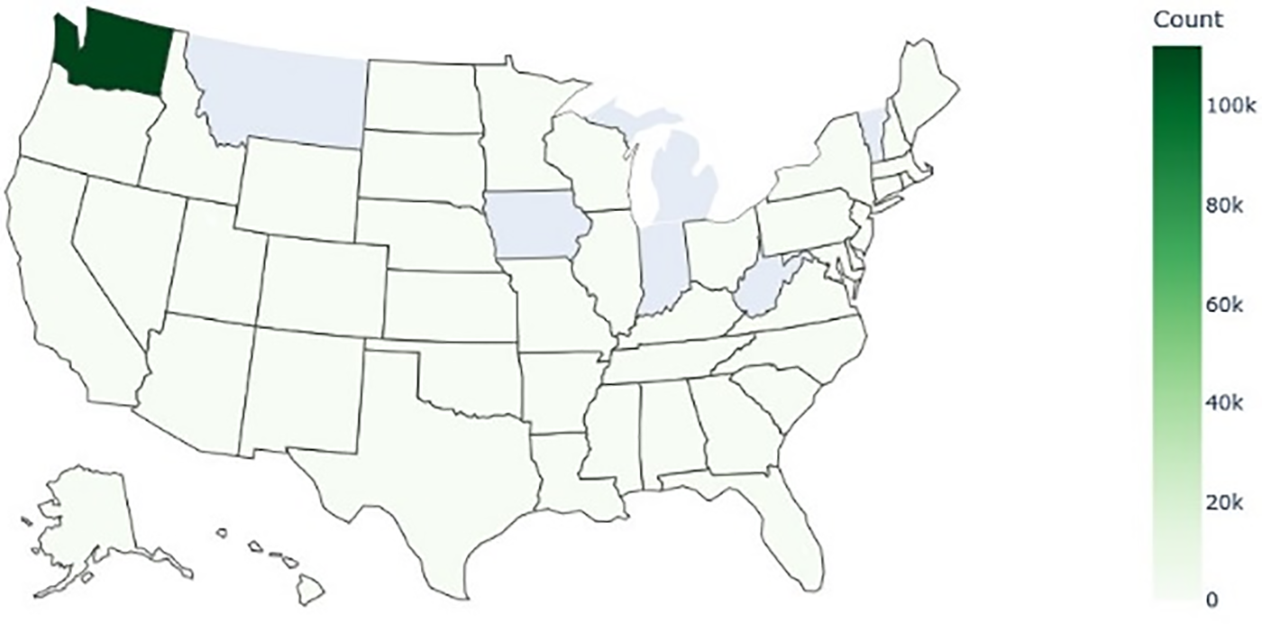
Figure 1: The prediction dataset shows BEV and PHEV distribution in the state

4.2 Feature Selection Results

Table 1 reviews binary optimization methods across multiple criteria. Each algorithm—bGGO, bGA, bPSO, bWOA, bGWO, and bFA—is evaluated using key markers for optimization efficiency. bGGO has the lowest “Average Error” value, indicating better convergence to optimal solutions. This shows that bGGO approximates the true solution better than other algorithms. The “Average Select Size” measure shows algorithm convergence. BGA has the shortest average select size, indicating a more focused optimization search. However, bWOA’s average choice size is substantially higher, meaning deeper solution space investigation. This statistic measures the “Average Fitness” of solutions. GGO and bGA have competitive average fitness, but bFA is behind. This shows that bFA solutions optimize less well.

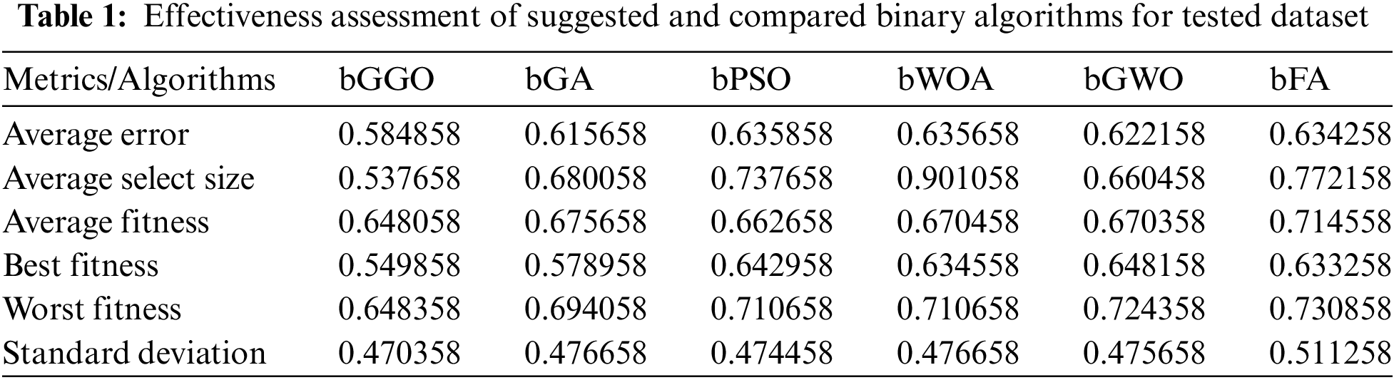
The lowest “Best Fitness” statistic shows bGGO can find high-quality solutions. BGA carefully selects the fittest runs. BFA’s slowness emphasizes its bad performance. “Worst Fitness” measures algorithm robustness. Again, bGGO shines with the lowest worst fitness value. This illustrates that bGGO’s least optimal solutions outperform others. The “Standard Deviation Fitness” indicator evaluates algorithm stability. Lower standard deviation values improve bGGO and bGA consistency during optimization runs. The standard deviation of bFA is bigger, indicating more solution unpredictability. bGGO uses targeted search despite having the lowest average error, highest fitness, and constant stability. Other algorithms like bPSO, bWOA, bGWO, and bFA have varied benefits and drawbacks, emphasizing the need to match the optimization problem. The average error of the proposed and compared binary algorithms for the assessed dataset is presented in Fig. 2. Fig. 3 shows binary GGO heatmap analysis, residual values, and approach comparisons.

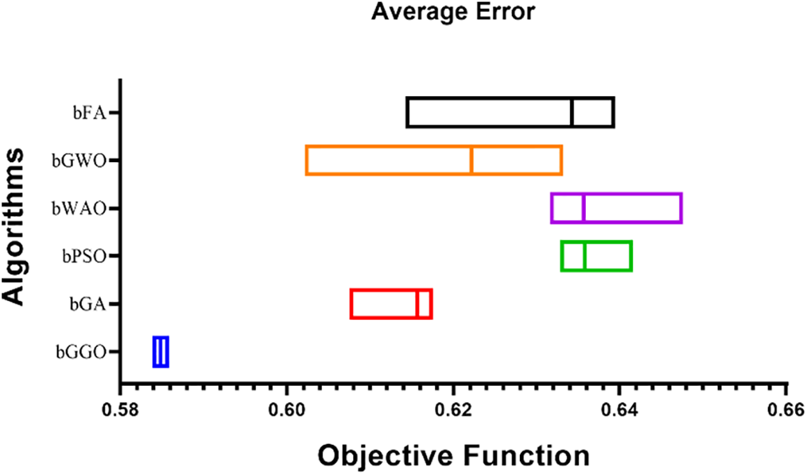
Figure 2: Average error of bGGO and compared binary algorithms for tested dataset

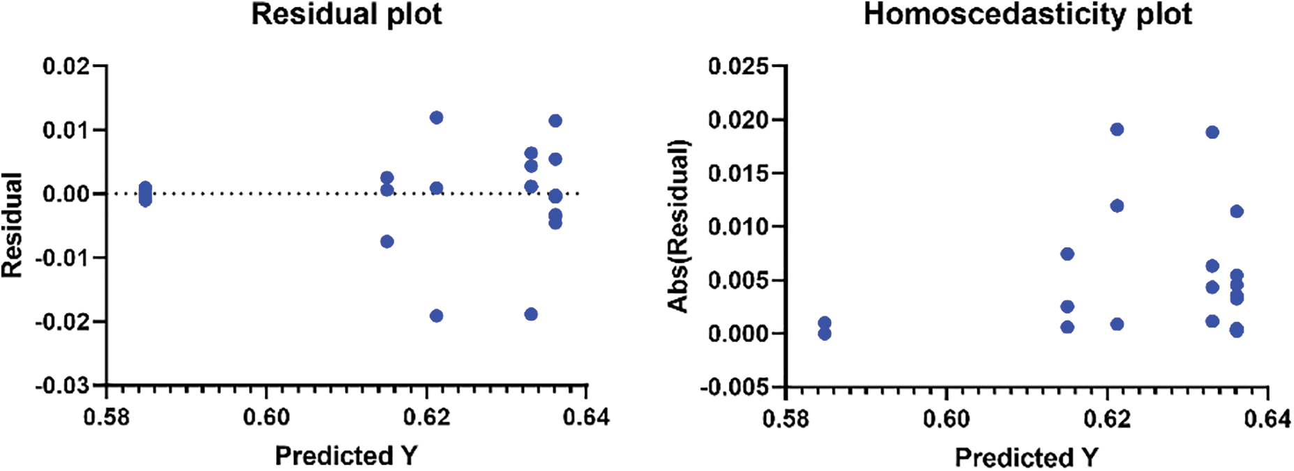
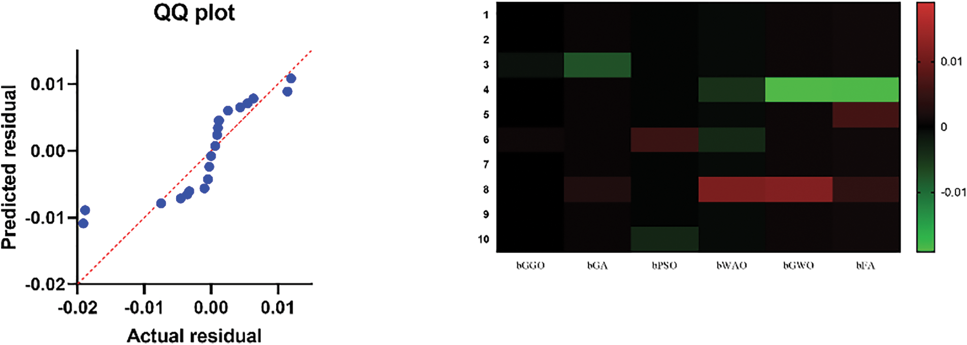
Figure 3: Residual values and heatmap analysis for binary GGO and compared algorithms

4.3 Classification Results

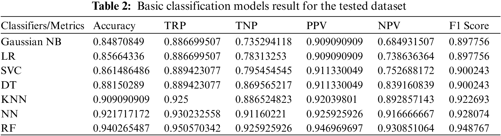
Table 2 shows categorization model performance metrics across evaluation criteria. To evaluate classification performance, Gaussian NB, Linear Regression (LR), SVC, Decision Tree (DT) Classifier, K-Neighbors Classifier (KNN), NN Classifier, and Random Forest (RF) Classifier are evaluated using key indicators. The Random Forest Classifier has the highest accuracy at 94.03%, followed by the NN Classifier at 92.17%. These models classify occurrences well, capturing many true positives and negatives. With a TRP of 92.50% and a TNP of 88.65%, K Neighbors Classifier succeeds at identifying positive and negative instances. Decision Tree Classifier has strong TRP and TNP, proving its sensitivity and specificity. Positive predictive value (PPV) measures precision, or the percentage of predicted positives that are correct. Random Forest Classifier has the highest PPV at 94.70%, followed by NN Classifier at 92.59%. These models excel in reducing false positives. The percentage of accurately anticipated negatives is called negative predictive value (NPV). Random Forest Classifier again performs well in NPV at 93.09%, demonstrating its capacity to recognize negative cases. Based on precision and recall, Random Forest Classifier has the highest F1 Score (94.88%), followed by NN Classifier (92.81%). These models balance precision and recall, making them suitable categorization candidates. Random Forest Classifier and NN Classifier lead numerous criteria with great accuracy, precision, and a balanced F1 Score. The best model may depend on interpretability, computational efficiency, and dataset properties.

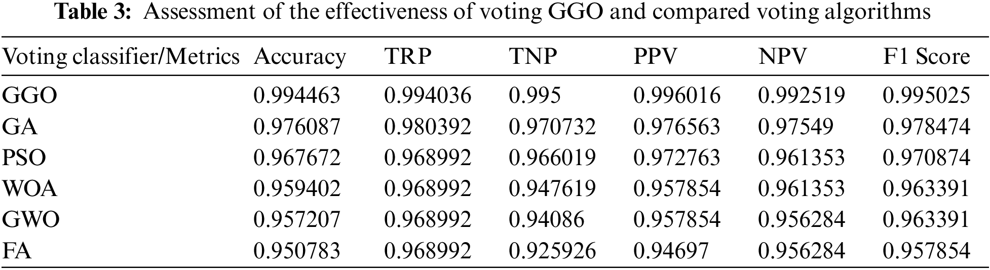
The results evaluate a Voting Classifier using GGO, GA, PSO, WOA, GWO, and FA optimization methods for important classification metrics, as presented in Table 3. The voting classifier is based on model predictions to decide, and the output indicates its performance. The voting GGO classifier has a remarkable 99.45% accuracy, which has the highest model accuracy, contributing to this success. This shows that the classifier’s accurate and robust classification is due to the models’ different predictions. Voting GGO is the best model, with a TRP of 99.40% and a TNP of 99.50%. This shows the voting GGO’s ability to detect positive and negative situations, which helps the classifier succeed. Voting GGO has the highest PPV of 99.60% and NPV of 99.25%, which reduces false positives and negatives. Voting GGO has the greatest F1 Score of 99.50%, which also indicates a balanced performance between precision and recall. Voting GGO’s contribution to the classifier’s success is further highlighted. Despite their lower individual accuracy, voting GA, PSO, WOA, GWO, and FA algorithms improve the voting classifier. This voting approach uses each algorithm’s skills to create a powerful, accurate, and robust classification model. The voting classifier, especially driven by the GGO algorithm, is a highly accurate classification solution with balanced performance across measures.

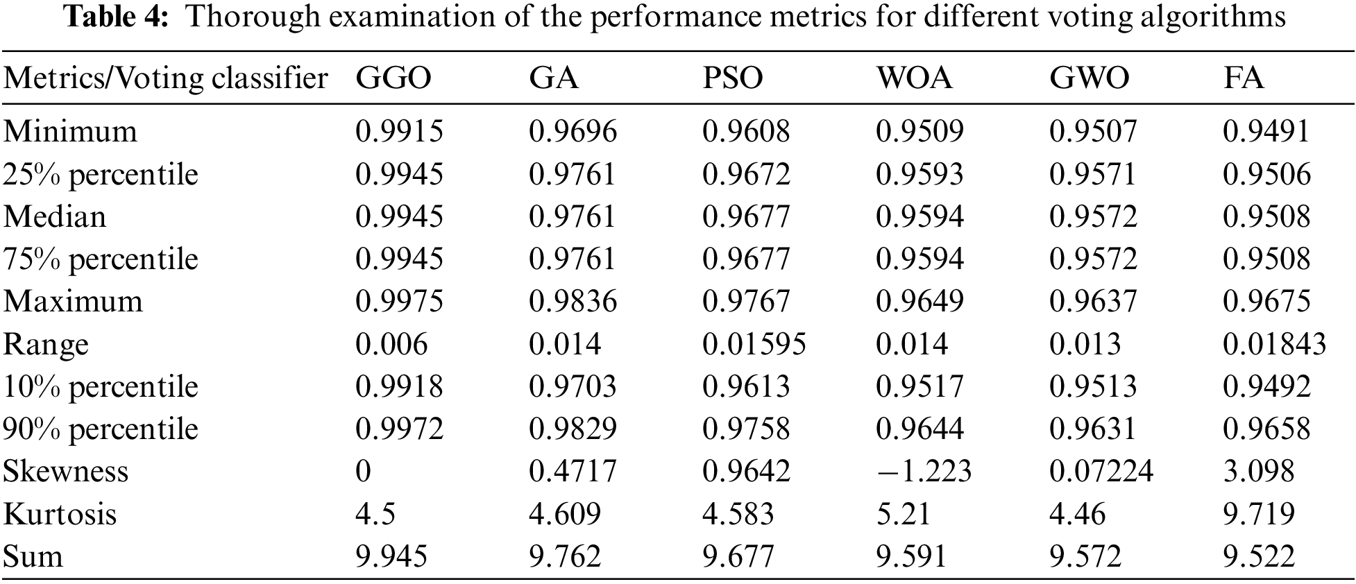
Based on numerical data, Table 4 shows the statistical performance of voting optimization algorithms of GGO, GA, PSO, WOA, GWO, and FA. Each voting algorithm’s minimum to maximum values shows its variability. The number of values for each algorithm is ten. Voting GGO has the narrowest range, showing dataset consistency. Data distribution is further defined by median and quartile values. Voting GGO routinely outperforms other algorithms with the highest median and lower quartiles. Voting GGO has the highest mean and lowest standard deviation, indicating stability and reliability, and regularly beats competing voting algorithms in these criteria, suggesting statistical robustness. Skewness and kurtosis provide distribution shape and tail characteristics. Voting GGO has a symmetric distribution (skewness near zero) and modest kurtosis, making it more normal than other methods. It performs well across statistical parameters like mean, median, confidence intervals, and distribution shape, making it a consistent and trustworthy optimization technique. These results indicate that voting GGO is reliable for numerical optimization.

After the completion of the earlier experiment, various voting classifiers, such as GGO, GA, PSO, WOA, GWO, and FA, were investigated when applied to the previously described dataset. The main objective was to assess and compare the levels of accuracy demonstrated by each approach. As depicted in Fig. 4, the results reveal that the GGO voting algorithm outperforms alternative solutions, displaying a significantly higher accuracy rate than the other options.

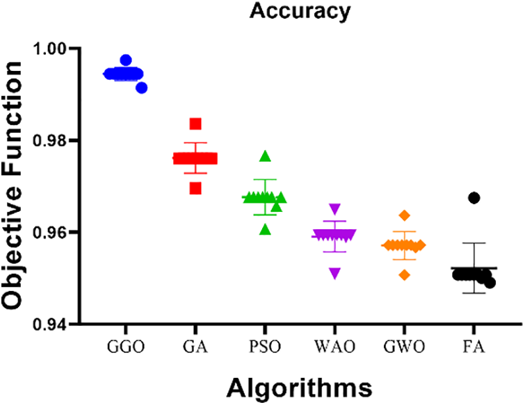
Figure 4: Assessment of the accuracy of voting GGO and compared models

In the upcoming experiment, we will explore how different voting algorithms demonstrate diverse levels of accuracy. Employing a methodology involving ten repetitions of the experiment and presenting the outcomes in the form of a histogram allows us to determine an average. The data gathered from each iteration of the experiment is illustrated in Fig. 5, offering a visual representation of the distribution of accuracy across multiple repetitions. The experiments compute residual values and heat and display the results in charts and comparisons. The residual values are graphed on a scattered, column-grouped y-axis during the initial computation. Fig. 6 shows the residual value distribution. QQ plots determine the similarity between expected and actual residual values. This graphic shows that the two sets of values match closely. Fig. 6 shows the homoscedasticity plot used to compare group variances. This shows the groups’ consistent differences. A heatmap in Fig. 6 is also used to appropriately examine the dataset’s values. When combined, these investigations provide a comprehensive understanding of residual values, their distribution, and group variance, which improves experiment interpretation.

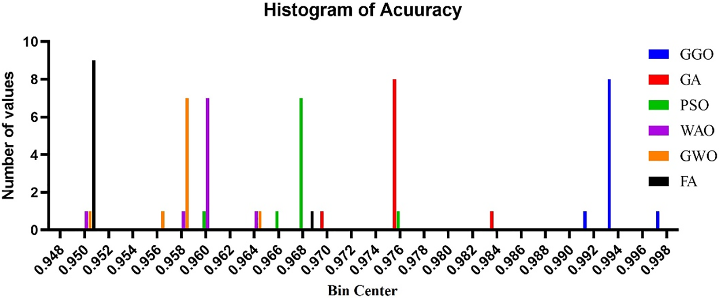
Figure 5: Exploration of the histogram of accuracy with bin center range of (0.948 0,998) for different voting classifiers

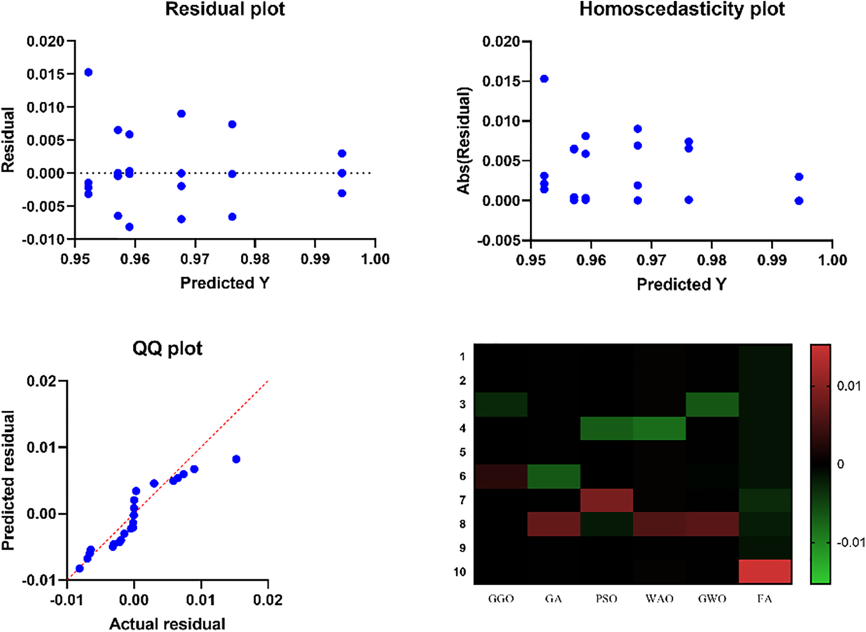
Figure 6: Residual values and heatmap analysis for voting GGO and compared models

4.4 Statistical Analysis

Table 5 compares the binary GGO (bGGO) algorithm to different binary optimization strategies using ANOVA. The analysis breaks variance into Treatment (between columns), Residual (within columns), and Total. The “Treatment” component, representing algorithm variability, yields a strong F-statistic of 173.4 for F (5, 54) and a low p-value (<0.0001), showing significant variances in algorithm group means. This implies that at least one algorithm performs significantly differently. Unexpected variation within each algorithm group is explained by the “Residual” component. The ANOVA results show that algorithm performance disparities are statistically significant, rejecting the null hypothesis of identical performance. This investigation illuminates binary optimization algorithm efficacy.

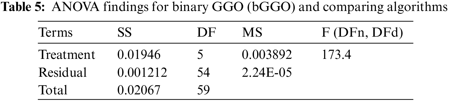
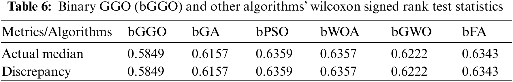
Table 6 presents the results of the Wilcoxon Signed Rank Test comparing the bGGO algorithm with other algorithms, namely bGA, bPSO, bWOA, bGWO, and bFA. The theoretical median for all algorithms is set at 0, and the actual medians for each algorithm are provided. The number of values is set to be ten for each algorithm. The test statistics include the sum of signed ranks (W), sum of positive ranks, and sum of negative ranks, all of which are equal at 55. The two-tailed p-values for each comparison are consistently low at 0.002, indicating a statistically significant difference between bGGO and each of the other algorithms. The discrepancy values highlight the magnitude of the differences in medians between bGGO and the other algorithms. In summary, the Wilcoxon Signed Rank Test results indicate that bGGO significantly outperforms each of the compared algorithms, with a substantial and statistically significant discrepancy in median values.

The ANOVA results in Table 7 compare the performance of a voting technique using the GGO algorithm to others. The analysis breaks variance into Treatment (between columns), Residual (within columns), and Total. The “Treatment” component, representing algorithm group variability, has a significant F-statistic of 187.7 for F (5, 54) and a low p-value (<0.0001). This shows large algorithm group mean disparities, rejecting the null hypothesis of equal performance. Each algorithm group’s “Residual” component represents unexplained unpredictability. The ANOVA results demonstrate the statistical significance of algorithm performance differences, proving at least one algorithm is better in the voting process. This investigation sheds light on voting algorithm performance.

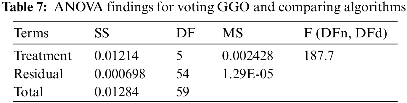
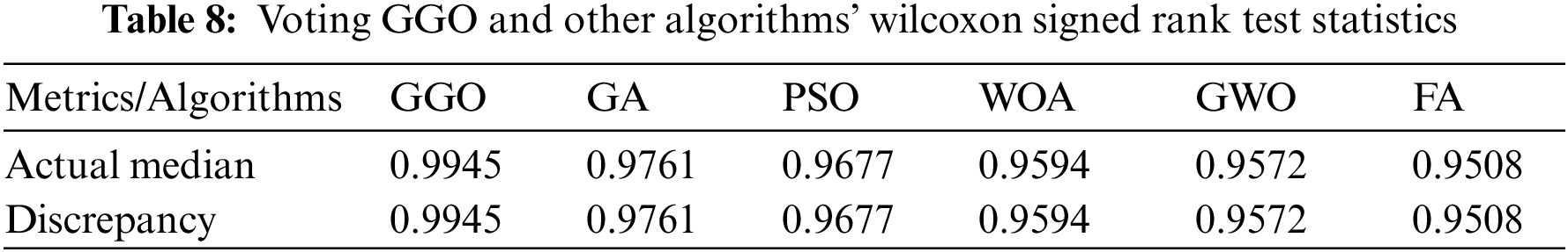
Table 8 compares the voting GGO algorithm to GA, PSO, WOA, GWO, and FA using the Wilcoxon Signed Rank Test. The theoretical median for all methods is 0, while the actual medians are presented. The number of values is set to be ten for each algorithm. Test statistics like the sum of signed ranks, positive ranks, and negative ranks are always 55. All two-tailed p-values for each comparison are 0.002, showing a statistically significant difference between the voting GGO algorithm and the others. The exact test was used, and the p-value summary shows “**”. The discrepancy numbers show how much the voting GGO algorithm’s medians deviate from the others. In conclusion, the Wilcoxon Signed Rank Test shows that the voting GGO algorithm surpasses all other algorithms with a large and statistically significant median difference.

By contributing to the optimization of charging infrastructure for electric vehicles, this work can play a crucial role in advancing the global transition to a low-carbon transportation system, which can also be aligned with climate change mitigation goals. The optimization of charging infrastructure stands to mitigate air pollution in some urban areas, which promotes the use of electric vehicles that are already known for lower emissions and, in turn, improve air quality and public health. The work also addresses energy-related concerns by positioning charging stations, which offer demand control through metaheuristic optimization algorithms. It could reduce the electricity expenses for consumers during peak hours. The optimization of electric vehicle charging infrastructure holds promise for significant societal advantages, including enhanced air quality, improved public health, emission reduction, and potential energy cost savings.

5  Conclusion and Future Directions

Finally, this study tackles the urgent need for sustainable mobility by examining the broad adoption of electric cars (EVs) and the constraints of urban charging infrastructure. The research emphasizes the need to overcome range and recharge time issues to promote EVs due to conventional transportation’s environmental impacts. Urban charging stations with fast and ultra-fast connectors are crucial. However, the research notes that high energy needs and service quality issues make powering these stations difficult. The study suggests a model that estimates each charging station’s maximum hourly capacity based on its geographic location to better estimate resource needs. This paper uses the binary graylag goose optimization (bGGO) algorithm for feature selection and the GGO approach for voting classifier and charging station demand allocation. The cost of traffic congestion is an important factor in decision-making. The study uses statistical analysis, including ANOVA and the Wilcoxon Signed Rank Test, to understand dataset variability and evaluate algorithm performance. Results demonstrate the Voting GGO algorithm allocates charging station demand well. A comparison with other optimization algorithms, such as the voting grey GWO, voting PSO, voting WOA, voting FA, and voting GA, sheds light on sustainable transportation and charging infrastructure planning in the future, emphasizing the need for tailored approaches based on regional traffic dynamics and effective algorithmic decision-making to meet the demands of a rapidly evolving transportation and charging infrastructure. More powerful evolutionary computation algorithms, such as learning-aided evolutionary optimization (LEO), will be studied and applied in the future for the charging station demand allocation of electric cars.

Acknowledgement: The authors confirm that this research project was funded by the Deanship of Scientific Research, Princess Nourah bint Abdulrahman University, through the Program of Research Project Funding after publication.

Funding Statement: This research project was funded by the Deanship of Scientific Research, Princess Nourah bint Abdulrahman University, through the Program of Research Project Funding After Publication, Grant No. (44-PRFA-P-48).

Author Contributions: The authors confirm contribution to the paper as follows: study conception and design: El-Sayed M. El-kenawy, Marwa M. Eid; data collection: Doaa Sami Khafaga; analysis and interpretation of results: Abdelhameed Ibrahim, Amel Ali Alhussan; draft manuscript preparation: Abdelhameed Ibrahim. El-Sayed M. El-kenawy. All authors reviewed the results and approved the final version of the manuscript.

Availability of Data and Materials: The data that support the findings of this study are openly available in data.wa.gov at https://catalog.data.gov/dataset/electric-vehicle-population-data (accessed on 20/03/2024).

Conflicts of Interest: The authors declare that they have no conflicts of interest to report regarding the present study.

References

1. A. Ibrahim et al., “A recommendation system for electric vehicles users based on restricted Boltzmann machine and waterwheel plant algorithms,” IEEE Access, vol. 11, pp. 145111–145136, 2023. doi: 10.1109/ACCESS.2023.3345342. [Google Scholar] [CrossRef]

2. M. A. Saeed et al., “A novel voting classifier for electric vehicles population at different locations using Al-Biruni earth radius optimization algorithm,” Front. Energy Res., vol. 11, pp. 1221032, 2023. doi: 10.3389/fenrg.2023.1221032. [Google Scholar] [CrossRef]

3. M. Ahmadi, K. Kazemi, A. Aarabi, T. Niknam, and M. S. Helfroush, “Image segmentation using multilevel thresholding based on modified bird mating optimization,” Multimed. Tools Appl., vol. 78, no. 1, pp. 23003–23027, 2019. doi: 10.1007/s11042-019-7515-6. [Google Scholar] [CrossRef]

4. W. Y. Lin, “A novel 3D fruit fly optimization algorithm and its applications in economics,” Neural Comput. Appl., vol. 27, no. 5, pp. 1391–1413, 2016. doi: 10.1007/s00521-015-1942-8. [Google Scholar] [CrossRef]

5. X. Wang, T. M. Choi, H. Liu, and X. Yue, “A novel hybrid ant colony optimization algorithm for emergency transportation problems during post-disaster scenarios,” IEEE Trans. Syst., Manage., Cybern. Syst., vol. 48, no. 4, pp. 545–556, 2018. doi: 10.1109/TSMC.2016.2606440. [Google Scholar] [CrossRef]

6. R. V. Rao and G. G. Waghmare, “A new optimization algorithm for solving complex constrained design optimization problems,” Eng. Optim., vol. 49, no. 1, pp. 60–83, 2017. doi: 10.1080/0305215X.2016.1164855. [Google Scholar] [CrossRef]

7. Z. G. Chen, Z. H. Zhan, S. Kwong, and J. Zhang, “Evolutionary computation for intelligent transportation in smart cities: A survey [Review article],” IEEE Comput. Intell. Mag., vol. 17, no. 2, pp. 83–102, 2022. doi: 10.1109/MCI.2022.3155330. [Google Scholar] [CrossRef]

8. J. Kennedy and R. Eberhart, “Particle swarm optimization,” in Proc. Int. Conf. Neural Netw., Perth, WA, Australia, 1995, vol. 4, no. 6, pp. 1942–1948. doi: 10.1109/ICNN.1995.488968. [Google Scholar] [CrossRef]

9. S. Mirjalili and A. Lewis, “The whale optimization algorithm,” Adv. Eng. Softw., vol. 95, pp. 51–67, 2016. doi: 10.1016/j.advengsoft.2016.01.008. [Google Scholar] [CrossRef]

10. S. Mirjalili, S. M. Mirjalili, and A. Lewis, “Grey wolf optimizer,” Adv. Eng. Softw., vol. 69, no. 1, pp. 46–61, 2014. doi: 10.1016/j.advengsoft.2013.12.007. [Google Scholar] [CrossRef]

11. H. Holland, “Genetic algorithms,” Sci. Am., vol. 267, no. 1, pp. 66–73, 1992. doi: 10.1038/scientificamerican0792-66. [Google Scholar] [CrossRef]

12. E. H. Houssein, D. Oliva, N. A. Samee, N. F. Mahmoud, and M. M. Emam, “Liver cancer algorithm: A novel bio-inspired optimizer,” Comput. Biol. Med., vol. 165, pp. 107389, 2023. doi: 10.1016/j.compbiomed.2023.107389. [Google Scholar] [PubMed] [CrossRef]

13. Z. H. Zhan, J. Y. Li, S. Kwong, and J. Zhang, “Learning-aided evolution for optimization,” IEEE Trans. Evol. Comput., vol. 27, no. 6, pp. 1794–1808, 2023. doi: 10.1109/TEVC.2022.3232776. [Google Scholar] [CrossRef]

14. E. S. M. El-Kenawy, N. Khodadadi, S. Mirjalili, A. A. Abdelhamid, M. M. Eid and A. Ibrahim, “Greylag goose optimization: Nature-inspired optimization algorithm,” Expert. Syst. Appl., vol. 238, no. Part E, pp. 122147, 2024. doi: 10.1016/j.eswa.2023.122147. [Google Scholar] [CrossRef]

15. M. H. Amini, M. P. Moghaddam, and O. Karabasoglu, “Simultaneous allocation of electric vehicles’ parking lots and distributed renewable resources in smart power distribution networks,” Sustain. Cities Soc., vol. 28, pp. 332–342, Jan. 2017. doi: 10.1016/j.scs.2016.10.006. [Google Scholar] [CrossRef]

16. A. El-Zonkoly and L. D. S. Coelho, “Optimal allocation, sizing of PHEV parking lots in distribution system,” Int. J. Electric. Power Energy Syst., vol. 67, pp. 472–477, May 2015. doi: 10.1016/j.ijepes.2014.12.026. [Google Scholar] [CrossRef]

17. L. Chen, C. Xu, H. Song, and K. Jermsittiparsert, “Optimal sizing and sitting of EVCS in the distribution system using metaheuristics: A case study,” Energy Rep., vol. 7, pp. 208–217, Nov. 2021. doi: 10.1016/j.egyr.2020.12.032. [Google Scholar] [CrossRef]

18. S. R. Gampa, K. Jasthi, P. Goli, D. Das, and R. C. Bansal, “Grasshopper optimization algorithm based two stage fuzzy multiobjective approach for optimum sizing and placement of distributed generations, shunt capacitors and electric vehicle charging stations,” J. Energy Storage, vol. 27, pp. 101117, 2020. doi: 10.1016/j.est.2019.101117. [Google Scholar] [CrossRef]

19. Data.wa.gov, Department of licensing, “Electric vehicle population data,” May 24, 2024. Accessed: Dec. 22, 2023. [Online]. Available: https://catalog.data.gov/dataset/electric-vehicle-population-data [Google Scholar]

20. M. Shibl, L. Ismail, and A. Massoud, “Machine learning-based management of electric vehicles charging: Towards highly-dispersed fast chargers,” Energies, vol. 13, no. 20, pp. 5429, 2020. doi: 10.3390/en13205429. [Google Scholar] [CrossRef]

21. M. Ahmed, Z. Mao, Y. Zheng, T. Chen, and Z. Chen, “Electric vehicle range estimation using regression techniques,” World Electric. Veh. J., vol. 13, no. 6, pp. 105, 2022. doi: 10.3390/wevj13060105. [Google Scholar] [CrossRef]

22. H. Kwon, “Control map generation strategy for hybrid electric vehicles based on machine learning with energy optimization,” IEEE Access, vol. 10, pp. 15163–15174, 2022. [Google Scholar]

23. M. O. Oyedeji, M. AlDhaifallah, H. Rezk, and A. A. A. Mohamed, “Computational models for forecasting electric vehicle energy demand,” Int. J. Energy Res., vol. 2023, no. 1934188, pp. 1–16, 2023. doi: 10.1155/2023/1934188. [Google Scholar] [CrossRef]