The Lightweight Edge-Side Fault Diagnosis Approach Based on Spiking Neural Network

1  Introduction

In the context of the Internet of Things (IoT), edge networks typically include edge devices and servers. The distribution of edge devices is often broad and diverse, covering environments such as homes, offices, industries, and cities [1]. Edge devices, including sensors, smartphones, smart home devices, and industrial robots, face various environmental challenges, such as temperature changes, humidity, vibration, etc. Due to the large number and wide distribution of edge devices, timely and effective network fault diagnosis becomes crucial. Rapid network fault diagnosis and resolution help reduce service interruption time, improve network reliability and stability, and ensure the normal operation of edge networks.

High real-time requirements are often required because of the substantial quantity of edge devices in edge networks. However, the traditional network fault diagnosis methods have the disadvantage that the edge devices send data to the edge server for processing [2], which leads to network latency. Especially under heavy network loads or unstable connections, this can result in slower network fault diagnosis. High real-time performance is crucial in some scenarios, such as intelligent Internet of Things (IoT), autonomous vehicles, and industrial IoT [3]. A direct network fault diagnosis on edge devices is necessary to address these challenges. The network fault diagnosis approaches enable edge devices to monitor and analyze their local data without relying on a central server and reduce the data transfer times and the network latency. Additionally, localized processing significantly enhances the real-time efficiency of the network fault diagnosis. Moreover, edge devices often face resource constraints, such as limited computing power, storage capacity, and network bandwidth in edge networks. Therefore, it is imperative to implement lightweight processing for fault diagnosis models in edge networks. This approach optimizes the utilization of edge device resources and prevents resource wastage or overload.

Traditional neural network models are typically complex and demand substantial computing resources, which makes them unsuitable because of the resource constraints in edge networks. For instance, Convolutional Neural Networks (CNNs) were widely used in image and speech recognition [4]. CNNs consist of multiple convolutional and pooling layers, which require significant computing resources for training. Deploying CNN models on edge devices for network fault diagnosis may exceed device computing capacities and storage space for model parameters. Hence, it is necessary to investigate the lightweight neural network model designed specifically for edge networks. Because of the complexity challenge of traditional neural network models, lightweight methods are essential to reduce the model size and computational complexity. Lightweight methods can enable their adaptability to edge device resource constraints. Due to their complexity, traditional neural network models are inappropriate for network fault diagnosis in edge networks. However, Spiking Neural Networks (SNNs) usually have a reduced model size and fewer parameters [5]. First, SNNs adopt an event-driven calculation method, calculating when the spike is received. SNNs can save energy, respond more quickly to the input spike signal, and process time-related information more efficiently. It is very suitable for edge networks of constrained resources and can require a fast response. Secondly, SNNs adopt a sparse coding method, meaning only some neurons will activate and generate pulses. This sparse coding method can reduce the demand for computing resources and storage space. Hence, it is suitable for the resource-limited situation of edge devices. Finally, the connection weights between SNN neurons are adaptive to better adapt to the complex edge networks.

Therefore, we propose the lightweight edge-side fault diagnosis approach based on Spiking Neural Network (LSNN) to satisfy the demands of high real-time and lightweight performance. This method not only maintains state-of-the-art accuracy but also diminishes the fault diagnosis model’s computational complexity.

(1) We use the modified Izhikevich neurons model to replace the Leaky Integrate and Fire (LIF) neurons model in LSNN. Izhikevich neurons inherit the simplicity of LIF neurons but also possess richer behavioral characteristics and the flexibility to handle diverse data inputs. Inspired by Fast Spiking Interneurons (FSIs) with a high-frequency firing pattern, we use the parameters of FSIs. Aside from enhancing the accuracy of network fault diagnosis, they are more suitable for edge network scenarios with multiple edge devices.

(2) Inspired the connection mode based on spiking dynamics in the basal ganglia (BG) area of the brain, we propose the pruning approach based on the FSIs of the BG in LSNN to improve computational efficiency and reduce the demand for computing resources and energy consumption.

(3) We propose a multiple iterative dynamic Spike Timing Dependent Plasticity (DSTDP) algorithm to enhance the accuracy of LSNN. DSTDP algorithm makes it more suitable for resource-constrained edge networks. Firstly, we adjust the connection weights using the DSTDP method before pruning to improve the learning ability and the accuracy of LSNN network fault diagnosis. After pruning, LSNN is fine-tuned again using the DSTDP method, allowing the network to relearn and adjust the weights of the remaining connections to maintain the LSNN’s performance.

The remainder of this article is structured as follows. In the section on related works, we discuss the current situation of network fault diagnosis, lightweight algorithms, and SNN. In the part of the proposed algorithm, we suggest the lightweight edge-side fault diagnosis approach based on a spiking neural network (LSNN). In the part of experiments, we analyze the efficiency and accuracy of the LSNN algorithm proposed and give some illustrative numerical results. Finally, the conclusion part summarizes this paper.

2  Related Work

Driven by the integrated innovation of intelligent manufacturing, industrial big data, and Industry 4.0, more and more edge devices have real-time data processing capabilities, reducing the reliance on central servers [6]. Unfortunately, various network faults inevitably occur during the operation of edge devices. These faults can result in system crashes, disrupt services, impact production and operations, and ultimately result in economic losses or even casualties [7]. Therefore, it is essential to promote the network fault diagnosis method in the edge networks and make accurate judgments and timely responses.

Over the years, through the wisdom and efforts of researchers, While network fault diagnosis methods have made some progress, fault diagnosis methods for edge networks are still in the early stages of research. Traditional network fault diagnosis methods can be categorized into three groups. Such as rule-based fault diagnosis methods [8], statistical analysis-based fault diagnosis methods [9], and machine learning-based fault diagnosis methods [10]. The rule-based fault diagnosis methods employ predefined rules to diagnose network faults. It can identify network faults quickly and easily but cannot deal with complex and obscure fault modes. The statistical analysis-based methods need to gather extensive data during network operation to analyze the characteristics of various network faults statistically. It is suitable for diagnosing large-scale network unknown faults and relatively complex fault modes. However, it has high requirements for data quality. Commonly used statistical methods include Bayesian network [11], cluster analysis [12], association rule analysis [13], and so on. As a typical representative of data-driven methods, machine learning-based fault diagnosis methods are a hot spot in the development of all walks of life. Classical, traditional machine learning models like Support Vector Machines (SVM) [14]. These traditional machine-learning models often require manual feature extraction and selection. These models need to be better suited for analyzing complex network fault data. Moreover, they need help extracting high-dimensional features due to their shallow structure.

With the increase in sensor diversity and scene complexity, a large number of different types of data are generated. Hence, it is difficult for traditional machine learning algorithms to obtain satisfactory diagnostic results. As the most eye-catching branch of machine learning, deep learning has made significant advancements in various fields, including image recognition, speech processing, and industrial fault diagnosis [15]. This is not only due to its internal advantages, such as automatic feature learning ability and powerful large-scale data processing ability. We also can not ignore the influence of external factors, especially the scale and complexity of network data, which has increased because of the rapid advancement of the industry. Of course, over the last five years, deep learning has propelled rapid development in intelligent fault diagnosis, including Deep Neural Networks (DNNs) [16], Long Short Term Memory networks (LSTM) [17], Recurrent Neural Networks (RNN) [18], Convolutional Neural Networks (CNN) [19], Graph Neural Networks (GNN) [20] and others. Considering that the time delay of network faults impacts the performance of fault diagnosis, Pan et al. [21] proposed an innovative fault diagnosis method based on the combination of CNN and LSTM. The CNN layer learning feature and LSTM layer capturing delay information of the model are combined to effectively improve the fault diagnosis performance. Chen et al. [22] proposed an interactive perceptual GNN (IAGNN) for diagnosing complex industrial process faults. The sensor signals are converted into heterogeneous graphs of various edge types, and fault features are extracted from each subgraph by multiple independent graph neural networks (GNN) blocks. The proposed method improves the fault diagnosis performance of complex industrial processes. Several deep learning approaches have gained remarkable consequences in intelligent fault diagnosis, yet they require significant computational power for training. Edge devices like IoT devices and smartphones are equipped with limited computational resources, making it challenging to directly execute complex deep learning algorithms. As an event-based computational model, spiking neural networks (SNNs) are rarely used in practical applications due to the challenge of supervised training and the non-differentiable nature of its peak activity. Additionally, SNNs have the advantages of saving energy and sparsity, so they are very suitable for resource-limited edge networks. SNN have shown great potential in edge networks and can realize intelligent fault diagnosis more effectively so as to promote its application and development in intelligent fault diagnosis.

In edge networks, the model using deep learning methods may be too complex, which is not conducive to real-time reasoning and processing on edge devices with limited computing power and storage resources. Hence, lightweight methods have emerged as a practical approach to tackling this issue. Weight sharing is an effective lightweight technique that significantly reduces the parameters and computational complexity of the model by sharing weight parameters among different layers of the model. Rothe et al. [23] utilized a shared encoder and decoder architecture to minimize memory footprint and achieved significant results in machine translation, text summarization, sentence segmentation, and sentence fusion. However, sharing the center layer weights can cause the model to perform poorly on different tasks. To solve this problem, Reid et al. [24] introduced a strategy called “sandwich” parameter sharing, which shares the weights of the central layer while maintaining the independence of the first and last layers. The method can be adjusted according to task specificity, thus ensuring the model performs well when dealing with different tasks. Nevertheless, with the increasing number of network layers, the model’s complexity also escalates, bringing significant training challenges. Aiming at problems like long-time training and significant consumption of computing resources in automatic speech recognition tasks, Takase et al. [25] studied the strategy of sharing weights across layers, allowing the weights of layer M to participate in the training of layer N at the same time. In this way, layer N can learn from the weight already trained by layer M, thus reducing the complexity of training and improving the efficiency of training. At the same time, this method also helps to accelerate the model’s convergence speed, enabling it to achieve superior performance quickly. At the same time, it can significantly reduce the training time and computing resource consumption. Another standard method of lightweight models is pruning, which removes unnecessary connections and parameters from the model. Therefore, this method can reduce the size and computation of the model. The existing model pruning methods are primarily used in machinery, image, speech, emotion, and text rather than in network faults. Zhang et al. [26] performed a single-time model pruning technique in neural networks and employed standard training to train the sparse network. This pruning method can decrease the model’s complexity in image recognition tasks. While one-time pruning may lead to a decline in the model’s accuracy after pruning, other iterative pruning strategies can be more flexible in choosing the timing and degree of pruning to maintain the performance in models better. The model is retrained by amplitude pruning [27], and the whole network is retrained by restoring the pruned parameters to obtain better performance and lower memory occupancy than the original model. In addition, the large scale of the pre-training network makes it difficult to deploy multiple tasks in a memory-limited environment, and the Diff adaptive pruning method [28] can enable parameters to carry out transfer learning efficiently and adapt to new tasks well. Meanwhile, Lagunas et al. [29] proposed a pruning method that considers blocks of various sizes, improving the model’s efficiency. Compared with other single pruning modes, Xia et al. [30] proposed a joint pruning method that can prune coarse-grained units and fine-grained units to better adapt to multi-task learning or multi-modal learning scenarios. More efficient pruning strategies are needed to enhance network fault diagnosis and management efficiency.

Spiking Neural Networks (SNN) have garnered considerable attention in recent years due to their high energy efficiency. It is suitable for resource-constrained edge networks that learn based on non-differentiated spike events and require less computational effort than back-propagation-based algorithms. Supervised SNN methods can roughly be divided into classic methods, the Back Propagation Through Time method (BPTT) and the Spike Timing Dependent Plasticity method (STDP). The former method requires continuous input data and is unsuitable for the event-driven SNN, while the latter STDP cooperates with the event-driven SNN. It can enable the network to learn and adapt to have more robust learning and memory capabilities according to the input timing information. In addition, memorized STDP behavior has also provided convergence in handwritten digit recognition [31]. In order to adapt different input patterns and learning tasks better, Hao et al. [32] proposed a symmetry Spike Timing Dependent Plasticity (sym-STDP) rule, which can further improve the model’s performance and generalization ability by combining the intrinsic plasticity of the biological synaptic scale and the dynamic threshold. Due to frequent memory access during training, Kim et al. [33] proposed a Time Step Spike Timing Dependent Plasticity (TS-STDP) that can minimize the storage size required for peak history. SNN, as a bio-inspired neural network, has become a research hot spot due to its advantages of energy saving, sparsity, time series information processing, and online learning. As a plasticity rule based on temporal correlation, STDP combines with the event-driven properties of SNN to further optimize the learning and computational performance of the network. In the future, with the further development of STDP and SNN technologies, they will play a more crucial role in artificial intelligence, providing powerful computing support for various practical applications in edge networks.

3  The Lightweight Edge-Side Fault Diagnosis Approach Based on Spiking Neural Network

3.1 Overview of the Overall Framework

Fault diagnosis is crucial for the uninterrupted and efficient operation of edge networks. Edge devices are equipped with limited computing power in edge networks, such as sensors or Internet of Things (IoT) devices. Due to the constrained computing resources of these edge devices, traditional deep learning methods often encounter challenges like model size, computational complexity, and power consumption. The lightweight edge-side fault diagnosis approach based on Spiking Neural Network (LSNN) is proposed to address the need for lightweight fault diagnosis in edge networks. This LSNN approach maintains higher accuracy while diminishing the computational complexity of other models compared to traditional SNN in fault diagnosis.

The general structure of LSNN is depicted in Fig. 1. First, a 3 × 3 convolutional layer is selected as the coding layer. Traditional neural networks often use large convolutional kernels, which increase the number of parameters and computational workload, leading to longer processing times. However, it is crucial for real-time data processing in edge networks and requires minimal delay to extract spatial features related to fault information. Therefore, inspired by the inception module, we apply two 1 × 1 and one 3 × 3 convolutional layers instead of a 7 × 7 convolutional kernel as coding layers. This helps in reducing the number of parameters in the convolutional layers. Secondly, the hidden layer serves as the SNN’s core and conducts signal processing and feature extraction for the timing characteristics of the received pulse signal. To improve LSNN model accuracy, we replace simple LIF neurons with Izhikevich neurons. It is known for its rich behavioral characteristics yet requires less computational effort. Additionally, we incorporate a max-pooling layer to preserve the original fault information characteristics, which enhances the LSNN’s ability to fit sequential tasks. This layer reduces the computational cost for subsequent layers, speeds up model training, and is particularly suitable for scenarios where edge network computing power is limited. Finally, the model concludes with a fully connected classifier for multi-class network fault diagnosis.

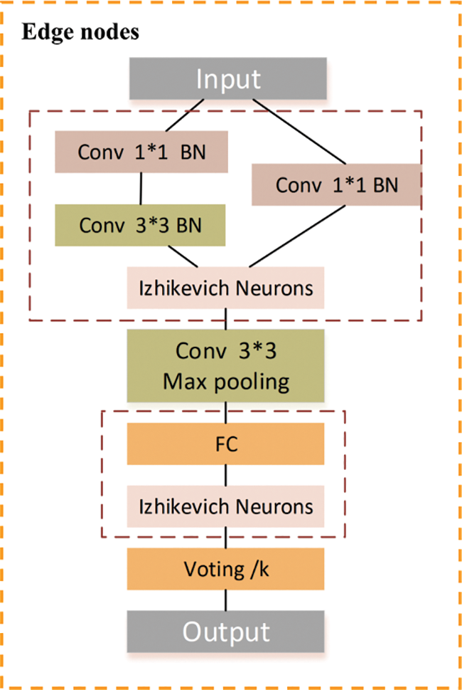
Figure 1: Overall framework of the lightweight edge-side fault diagnosis approach based on spiking neural network with Izhikevich neurons

3.2 The Izhikevich Neurons Model of the SNN

The Spiking Neural Network (SNN) is a computational model miming biological neural networks, with the neuron as its fundamental unit. The selection of neuron types significantly influences the performance and behavior of SNN. Research has identified three common types of neurons: The Leaky Integrate and Fire (LIF) model [34], the Izhikevich model [35], and the Hodgkin-Huxley (HH) [36] model. The LIF model has become the foundational neuron model in SNN due to its simplicity and ease of comprehension. Its primary advantage lies in effectively implementing pulse transmission and possessing inherent filtering characteristics, enhancing performance when processing external input signals. The Izhikevich model is a simple and robust neuron model capable of simulating various neuronal behaviors, such as spike firing patterns and action potential durations. Consequently, it holds significant practical value in exploring complex neural network behaviors. Compared to the LIF model, the Izhikevich model adapts better to diverse neural network scenarios with lower computational complexity. Lastly, the HH model is one of the most complex neuron models available, providing a more accurate simulation of neuronal activities in living organisms. By detailing ion channels, the HH model replicates the action potential generation and decay process with high precision. However, its intricate structure results in higher computational costs and limits its practical application scope in specific scenarios. These three neuron types exhibit distinct characteristics within pulsed neural networks, each suitable for different scenarios. The LIF model excels in simplicity and effectiveness in processing external signals, the Izhikevich model offers simplicity, versatility, and practical value across various neural network behaviors. In contrast, the HH model provides unparalleled accuracy at the cost of higher computational demands.

The LIF model is one of the fundamental computational units in SNN. It is widely used in other SNN models as well. This model is a simplified representation of biological neurons, capturing the nonlinear relationship between inputs and outputs. The subthreshold dynamics of LIF spiking neurons can be described as follows:

τdV(t)dt=−(V(t)−Vrest)+W(t)(1)

where V(t) is the membrane potential of the neuron at time t, W(t) is the weighted sum of the input spikes for each time step, Vrest is the resting potential and τ is the membrane time constant.

When the neuron receives input from the preceding layer, its membrane potential undergoes accumulation. Upon exceeding a specific threshold V(t) at time t, the neuron fires a spike, followed by the membrane potential V(t) returning to a reset value Vreset which is set to be 0 in this paper. The LIF neurons are at the extreme in computational cost, potentially sacrificing computational accuracy.

The HH model model is a fundamental mathematical framework for elucidating the initiation and propagation of action potentials within neurons. This pivotal model, crafted by Alan Hodgkin and Andrew Huxley in 1952, delves into the intricate interplay of ions traversing neuronal membranes via ion channels. At its core, the HH model is formulated with a collection of differential equations meticulously detailing the dynamics of both membrane potential and the gating variables intrinsic to ion channels. The membrane potential V of neurons using the HH model can be described as the following dynamics:

CmdVdt=I−g¯Nam3l(V−ENa)−g¯Kn4(V−EK)−g¯L(V−EL)(2)

where Cm represents the membrane capacitance of the neuron, V represents the membrane potential of the neuron, I represents the external stimulation current applied, g¯Na represents the maximum sodium conductance, m represents the activation gating variable of sodium channels, l represents the inactivation gating variable of sodium channels, ENa represents the sodium equilibrium potential, g¯K represents the maximum potassium conductance, n represents the activation gating variable of potassium channels, EK represents the potassium equilibrium potential, g¯L represents the leak conductance, EL represents the leak equilibrium potential.

These equations describe how the membrane potential V changes over time based on the flow of ions (sodium, potassium and leak) through voltage-gated channels. The gating variables m, l, and n describe the opening and closing of these channels, which in turn influence the membrane potential. The HH model provides a detailed and biophysically realistic representation of the neuronal membrane dynamics, allowing for the simulation of action potentials with high accuracy. However, the HH model involves a set of differential equations with multiple parameters, making it computationally intensive and complex.

Unlike the LIF and HH neurons models, we propose the Izhikevich neurons model which strikes a balance between computational efficiency and biological realism in the paper. The LIF model is characterized by its simplicity and commonality, but it may lack flexibility in handling certain neuronal behaviors. On the other hand, the HH model offers higher complexity and biological realism, but it comes with higher computational costs in practical applications. In contrast, the Izhikevich model combines simplicity, versatility and capable of simulating various neuronal behaviors including fast and slow spiking patterns. This makes the Izhikevich model a widely applicable and computationally efficient choice, particularly suitable for simulating large-scale neural networks.

The Izhikevich model simplifies neuronal dynamics into a two-dimensional system of ordinary differential equations, capturing essential features of neuronal behavior. Despite its simplicity, this model can emulate a broad spectrum of spiking patterns observed in biological neurons, such as regular spiking, fast spiking, bursting, and more. Its ability to simulate diverse neuronal behaviors makes it a valuable tool for studying neural networks. The dynamics of the membrane potential and the recovery potential in the Izhikevich model are governed by the following equations:

dvdt=0.04v2+5v+140−u+I(3)

dudt=a(bv−u)(4)

where v is the membrane potential of the neuron, u is the recovery potential, I is the external stimulation current, a and b are parameters controlling the dynamics of the recovery variable u, t represents time. These equations describe how the membrane potential and the recovery potential change over time due to input currents and intrinsic dynamics. Adjusting the parameters a and b allows for the simulation of various neuronal behaviors, providing a flexible and efficient framework for modeling neural networks.

As shown in Fig. 2, we simulated the firing patterns of individual neurons under different model parameters. Notably, FSIs exhibit notably high-frequency firing compared to the other neurons. This characteristic enables FSIs to generate a greater number of action potentials within shorter intervals, facilitating rapid encoding and transmission of input information. In contrast, neurons like TCs display relatively lower firing frequencies, suggesting they are not as swift or efficient as FSIs in information processing. The high-frequency firing mode of FSIs enhances the speed and efficiency of data processing, rendering it particularly well-suited for the demanding real-time constraints of edge networks. Therefore, FSIs are selected as the main neurons of our proposed LSNN model. As shown in Eqs. (6) and (7), the parameters u = 0, I = 5, a = 0.02, and b = 0.2 are set to simulate the high-frequency firing pattern of FSIs, thereby improving the computational efficiency of the model.

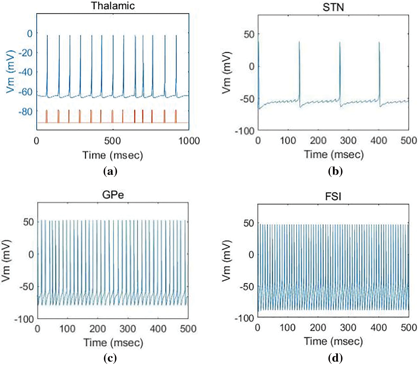
Figure 2: The firing patterns of individual neurons under different model parameters. (a) Thalamus neurons (TCs) and sensorimotor cortex (SMC) (b) Subthalamic neurons (STNs) (c) Globus pallidus Externa neurons (GPes) (d) Fast-spiking Interneurons (FSIs)

In practical applications, edge networks often require the processing of substantial real-time data. This necessitates adopting efficient and precise models in return for efficient and accurate data processing. The Izhikevich neurons model can rapidly simulate the spike patterns of biological neurons, which provides robust support for neural network applications in edge networks. Additionally, the future development of edge networks will exhibit a trend of diversification and complexity, resulting in the emergence of various types of edge devices. The Izhikevich neurons model demonstrates good scalability to adapt to future complex edge networks, which offer high flexibility and sustainability.

3.3 The Pruning Approach Based on Fast Spiking Interneurons (FSIs) of the Basal Ganglia in LSNN Model

The pruning method in Spiking Neural Network (SNN) is significant for enhancing computing efficiency, shrinking model size, optimizing real-time performance, boosting model reliability, conserving communication bandwidth, and aligning with edge-specific characteristics. The inter-neuronal connections are minimized, cutting computational complexity and conserving computational resources and energy through pruning. This optimization operation enhances the speed of the network’s real-time responsiveness and data processing. These benefits empower edge devices to run SNN models more efficiently, meeting the demands of real-time processing, low latency, and energy efficiency in edge networks.

The connectivity structure diagram of the Basal Ganglia is shown in Fig. 3, which reprinted with permission from [37]. The model primarily consists of subthalamic neurons (STNs), globus pallidus externa neurons (GPes), globus pallidus Interneurons (GPis), fast-spiking Interneurons (FSIs), D1 medium spine neurons (D1 MSNs), D2 medium spine neurons (D2 MSNs), thalamus neurons (TCs) and sensorimotor cortex (SMC). As depicted in Fig. 3, we observe distinct firing patterns among TCs, STNs, GPes, and FSIs. Notably, FSIs exhibit notably high-frequency firing compared to the other neurons. This characteristic enables FSIs to generate a greater number of action potentials within shorter intervals, facilitating rapid encoding and transmission of input information. In contrast, neurons like TCs display relatively lower firing frequencies, suggesting they are not as swift or efficient as FSIs in information processing. The high-frequency firing mode of FSIs enhances the speed and efficiency of data processing, rendering it well-suited for the demanding real-time constraints of edge networks.

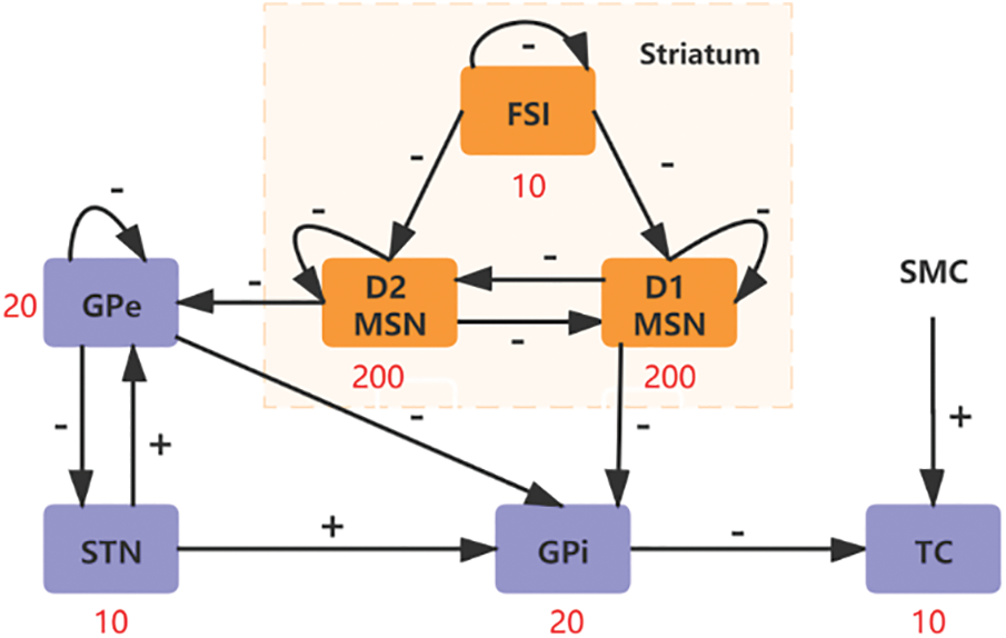
Figure 3: The connectivity structure diagram of the Basal Ganglia. The model primarily consists of subthalamic neurons (STNs), globus pallidus externa neurons (GPes), globus pallidus Interneurons (GPis), fast spiking Interneurons (FSIs), D1 medium spine neurons (D1 MSNs), D2 medium spine neurons (D2 MSNs), thalamus neurons (TCs) and sensorimotor cortex (SMC)

Therefore, FSIs are selected as the main neurons of our proposed LSNN model and the Izhikevich neurons model is adopted from Subsection 3.2. As shown in Eqs.(6) and (7), the parameters u = 0, I = 5, a = 0.02, and b = 0.2 are set to simulate the high-frequency firing pattern of FSIs, thereby improving the computational efficiency of the model. Additionally, we draw inspiration from the connectivity patterns of neurons in the BG of the brain and perform a pruning operation on LSNN to reduce the demand for computing resources and energy consumption by removing redundant connections.

The basal ganglia network model comprises GPes, STNs, GPis, D1 MSNs, D2 MSNs, FSIs, TCs and sensorimotor cortex (SMC) interconnected to create a network that processes input from the sensorimotor cortex [38]. The neurons in this network are linked in a sparse structured manner, which referred to as projection in spiking dynamics. This connectivity can be mathematically formulated as:

C∞(v)=11+exp⁡(−v+3015)(5)

where v represents the membrane potential of FSIs. We convert the network fault timing data into pulse signal input, which will eventually affect the membrane potential of FSIs.

To tackle the challenge of limited energy consumption of edge nodes in edge networks, the connection relationships among Izhikevich neurons are sparse. The input neurons x and the hidden neurons y are randomly sorted and numbered. The equation of the connection probability between neurons x and y is shown as follows:

pxy=11+exp⁡(−x−yx+y)(6)

Through the analysis above, when the connection relationships are sparse, the lightweight LSNN network structure can be achieved. Therefore, N is set as follows, indicating the upper limit for the connections of FSIs in LSNN:

N=⌈c1*c2*c⌉(7)

where c=2×10−5 represents the initial connection probability between neurons in LSNN, c1=128 denotes the count of neurons in the input layer, and c2=200 signifies the count of neurons in the hidden layer. The condition for an edge connection between neurons j and k in LSNN is defined as:

ejkexist wherepjk≥N(8)

As shown in Fig. 4, to explore the trade-offs between model complexity and performance, we systematically varied the pruning threshold and monitored the resultant changes in diagnostic accuracy and model size. Additionally, we identified a threshold N = 0.512 below, which further pruning deteriorates performance.

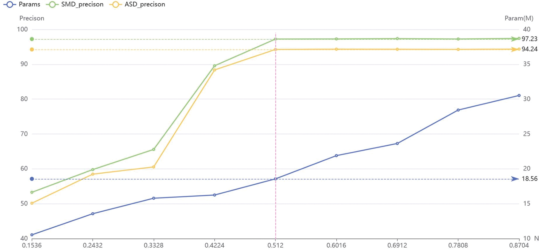
Figure 4: The effect of parameter N on precision and params in LSNN

Based on the above definition, spiking dynamics can enhance the neuron connection relationships in the LSNN. This method integrates relevant knowledge from spiking dynamics in biological neuroscience to tailor the LSNN network structure, achieving a lightweight effect for the temporal feature extraction model. The pseudocode of the pruning approach based on FSIs of the Basal Ganglia in the LSNN model is as follows:

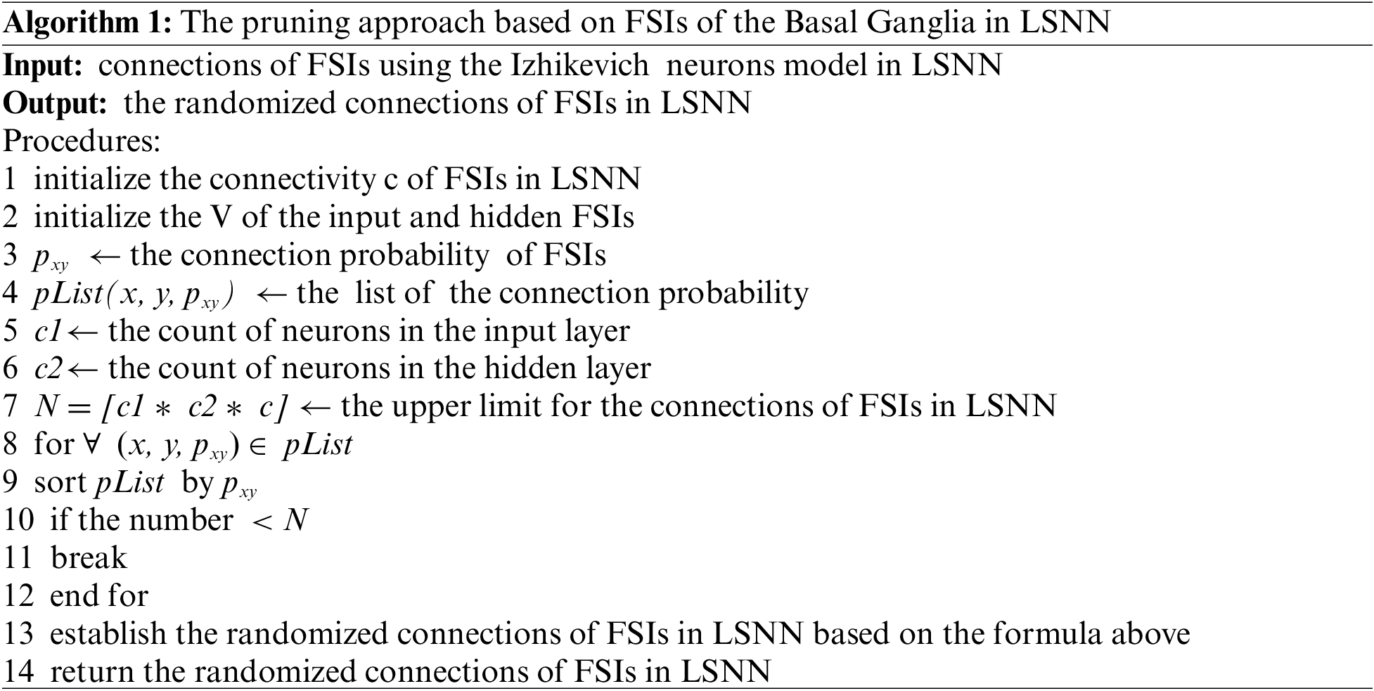
In edge networks, edge devices typically possess limited computing power and capacity due to their small size and power consumption constraints. Moreover, these edge devices are frequently utilized in real-time applications, such as IoT sensors and intelligent transportation systems, which demand rapid responses. These devices must process and respond to events almost instantaneously, such as monitoring temperature changes or detecting motion. Our proposed pruning method effectively reduces the complexity of the LSNN model, diminishes the demand for computing resources and energy consumption, and enhances the computational efficiency of LSNN. This refinement with superior performance allows for deployment in edge networks, enabling swift responses to specific tasks.

3.4 Dynamic STDP-Based Approach in LSNN Model

Spike Timing Dependent Plasticity (STDP) learning rule governs the evolution of connection strengths between neurons over time. The adjustment of synaptic weights is a crucial task in the training process of Spiking Neural Networks (SNNs). STDP is widely adopted as an unsupervised training algorithm [39] for SNNs as it allows the connections between neurons to adapt based on the timing of input signals, thereby optimizing the network. According to its hypothesis, the strength of a synapse depends on the difference in spike timing between the pre-neuron and post-neuron. The calculation for updating the weight of an individual synapse follows a power-law formula:

δw=η×[e(tpre; −tpost τ)−offset]×[wmax−w]μ(9)

where Δw represents changes in synaptic weight over time, η represents the learning rate, tpre represents the time of pre-synaptic spikes, tpost represents the time of post-synaptic spikes, τ represents the time constant, offset represents a constant variable used to counteract depression, wmax represents the upper limit restriction placed on the synaptic weight, w represents the weight value from the previous iteration, μ represents a constant that influences the exponential dependence on the previous weight value. As shown in Fig. 5, the updated weight increases if the post-neuron spikes immediately after the pre-neuron. On the contrary, the updated weight decreases if the spikes are far apart.

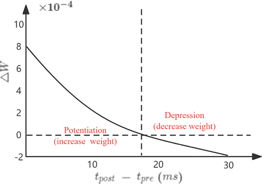
Figure 5: Modification of the synaptic weight between pre-synaptic and post-synaptic spikes over time. (η = 0.002, τ = 20 ms, offset = 0.4, wmax = 1, w = 0.5, μ = 0.9)

Pruning is a widely used optimization technique in machine learning aimed at reducing redundant parameters of the model. Pruning methods are effective in reducing model size and computational complexity while retaining the crucial structure of the network and performance. The integration of the STDP and pruning methods allows for dynamic adjustment of connection weights based on spike timing information between neurons, enabling the network to better capture temporal dependencies. Simultaneously, pruning techniques effectively eliminate unnecessary connections, leading to lighter models. In conclusion, we propose the dynamic STDP-based (D-STDP) pruning approach to get connection adjustment and weight quantization in LSNN in this paper. The proposed approach not only lightens the model but also enhances the accuracy of LSNN, making higher practical value in edge networks.

Specifically, the D-STDP approach, including training, pruning, and optimization phase to get connection adjustment and weight quantization in LSNN, can be divided into three steps as follows:

1.    Training phase: The STDP rule is employed to adjust connection weights of FSIs based on the spike timing information of the input data.

2.    Pruning phase: Following the training phase, the pruning approach based on biological fast-spiking Interneurons (FSIs) of the Basal Ganglia, as described in Subsection 3.3, is applied to LSNN. This step removes redundant connections, reducing the complexity and enhancing the computational efficiency of the LSNN model.

3.    Iterative optimization phase: The D-STDP approach is once again utilized to fine-tune connection weights between FSIs to lightweight LSNN after the pruning phase. This ensures that the pruned network maintains high performance.

Additionally, the proposed D-STDP method is used to train the weight of the excitatory synapses and classify them into critical and non-critical synapses. Synaptic inputs that have no contribution to learning remain the weights unchanged, serving as potential candidates for deletion, and are classified as non-critical synapses. Conversely, synapses with higher weights are more likely to have strong learning abilities and are classified as essential synapses. The entire training set is divided into batches to prune iteratively, and the weight of the non-critical synapses is reduced to 0 after each batch. The network then proceeds to the following processing batch, with the synapses having 0 weights continuing to participate in the training. Reducing weights to 0 rather than eliminating connections is crucial for learning the present inputs in subsequent batches. Eliminating non-critical synapses can lead to two undesirable consequences. Firstly, it hampers the network’s ability to learn new inputs. Secondly, it forces the network to forget previous inputs to make way for new ones. Therefore, the zero-weight strategy in neural network training achieves a balance between learning new and retaining old representations. This improves the flexibility and adaptability of LSNN, providing superior performance for edge networks dealing with complex tasks.

4  Experiment

4.1 Datasets Description

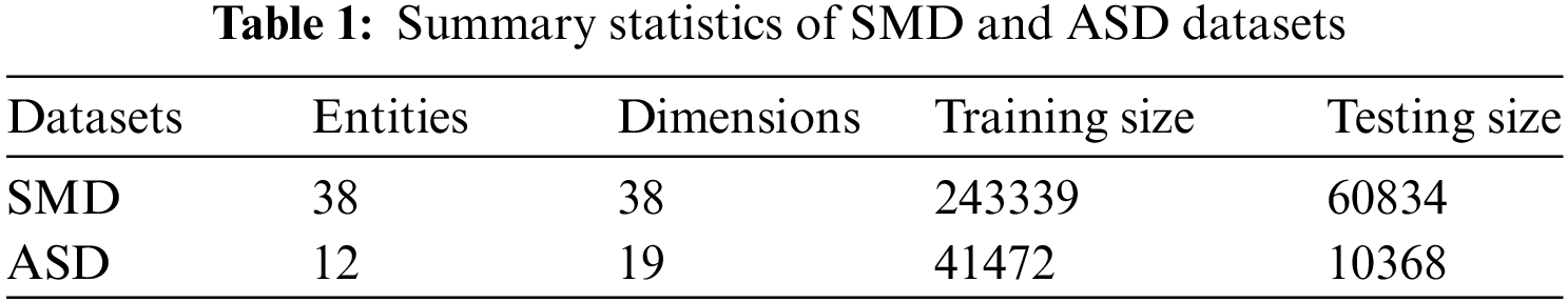
We verify the prediction effect of LSNN on two real network server datasets: The SMD (Server Machine Datasets) and ASD (Application Server Datasets) datasets. The two datasets are described as follows:

(1)   SMD [40] are new datasets spanning 5 weeks, collected from a major Internet company and publicly available on GitHub. The SMD datasets are split into two subsets, where 80% of the data set is used as the training set and 20% of the training set is used as the test set.

(2)   ASD [41] gathered from a prominent Internet company. The datasets comprise a set of stable services running on 12 entities representing the status of a server. More specifically, the ASD datasets include multivariate time series data during 45 days with 19 metrics describing the server’s performance. These metrics include CPU, memory, network, virtual machine and more. Observations in ASD are equally spaced 5 min apart. The ASD datasets are split into two subsets, where 80% of the data set is used as the training set and 20% of the training set is used as the test set.

The two datasets consist of observations are based on 1-min intervals. Meanwhile, Table 1 provides the name, the quantity of entities, dimensions, the training and testing sets of the two datasets.

4.2 Experiment Settings

Our experiments were conducted within a controlled software environment to ensure consistency and reproducibility. The experiments utilized a Dell server with two 2.90 GHz 64 Intel (R) Xeon (R) Gold 6226 R CPUs and four NVIDIA 3090 GPU cards. In addition, PyTorch 1.10.0 is used to build the deep neural network framework, Conda 4.9.2 is used as dependency management, Ubuntu 20.04 LTS is used as Operating System, and Python 3.7.12 is used as the programming environment.

The number of neurons in the input layer is 128 and the number of neurons in the hidden layer is 200. For the Izhikevich neuron parameter, the parameters u = 0, I = 5, a = 0.02, and b = 0.2 are set to simulate the high-frequency firing pattern of FSIs, thereby improving the computational efficiency of the model. In addition, our pruning method uses a specific threshold, N = 0.512, the D-STDP configuration includes the learning rate of 0.002, the upper limit restriction placed on the synaptic weight of 20 ms, the upper limit restriction placed on the synaptic weight of 1, a constant that influences the exponential dependence on the previous weight value of 0.9, with these parameters are fine-tuned for optimal performance.

To prepare the datasets for our experiments, we implemented several preprocessing steps to ensure data quality and model compatibility. Initially, we normalized each feature in the dataset to achieve a mean of 0 and a standard deviation of 1, ensuring a consistent scale across all input variables. Due to the imbalance in the representation of different fault types, we utilized synthetic data generation techniques to augment underrepresented classes, thereby enhancing the model’s ability to generalize across various fault conditions.

We compare our LSNN approach with the following baseline methods:

LSTM-NDT [42] is designed to address the complexity and variability of time series data in practical scenarios. It comprises an LSTM layer and a nonlinear dynamic threshold layer. During training, the LSTM layer learns the long-term and short-term dependencies of the time series data, while the nonlinear dynamic threshold layer dynamically adjusts the threshold based on the input data at the current time step.

MAD-GAN [43] focuses on the development of a novel anomaly detection approach using Generative Adversarial Networks (GANs) for multivariate time series data.

OmniAnomaly [40] focuses on the development of a novel approach for anomaly detection in multivariate time series data using Stochastic Recurrent Neural Networks (SRNN).

VAEpro [44] focuses on using Variational Autoencoders (VAEs) for anomaly detection and understanding which dimensions of the input data contribute most to detected anomalies.

SNN [5] is trained using the improved Spike Timing Dependent Plasticity (STDP) learning rule for fault diagnosis in the Bearing datasets. Additionally, the concept of time is introduced into the SNN model, which makes it with highly bio-inspired characteristics.

4.3 Algorithm Evaluation Metrics

To showcase the results of LSNN, we utilize three classic metrics to evaluate the proposed approach’s effectiveness: Precision, Recall, and F1. Precision represents the proportion of correct predictions made by LSNN out of all predicted results, reflecting the prediction accuracy of LSNN. Recall is the proportion of actual positive instances correctly predicted by LSNN out of all actual positive instances. F1 represents the harmonic mean of precision and recall used in classification problems. It provides a balance in terms of precision and recall to assess the algorithm’s performance. The actual positive rate represents the correctly diagnosed instances (i.e., the number of correctly diagnosed results). The false positive rate indicates an incorrect diagnosis of other categories as this category (i.e., the number of fault diagnoses to happen but do not happen actually). The false negative rate represents the diagnosis of other categories as this category (i.e., the quantity of events not diagnosed but happened). Additionally, to evaluate the complexity of LSNN, we use metrics like parametersb(Params) and floating-points (FLOPs) to evaluate the lightweight performance.

4.4 Experiment Results

The Experiment Results section evaluates the performance of the proposed LSNN method from multiple perspectives. Given the absence of an open-source fault diagnosis method specifically designed for various kinds of node faults, we compare our method with existing classification algorithms that have shown effectiveness in single-component fault diagnosis scenarios. This comparison highlights the advantages of our proposed method. We analyze the LSNN algorithm’s performance, where edge node devices’ computing and storage capacities are typically limited in the edge network. Considering these indicators, Precision, Recall, F1, Params, and FLOPs are crucial for evaluating the LSNN algorithm’s lightweight and accuracy performance.

4.4.1 Analysis of the Effectiveness in LSNN

To evaluate the accuracy performance of the proposed LSNN method, we selected five excellent algorithms for comparison, including the LSTM-NDT algorithm proposed in [42], the MAD-GAN algorithm proposed in [43], the OmniAnomaly algorithm proposed in [40], the VAEpro algorithm proposed in [44], the SNN algorithm proposed in [5].

Table 2 demonstrates the comparison of MRSTGCN and other baseline models of the indicators Precision, Recall, and F1 for the network fault diagnosis tasks. Specifically, the improvement effects are as follows.

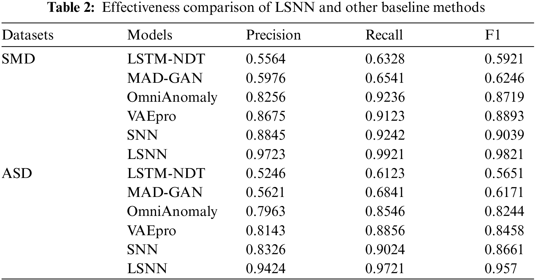
Our LSNN model proposed in this paper achieves optimal Precision, Recall and F1 on two datasets in Table 2. For the SMD datasets’ results, on the precision metric, the proposed LSNN algorithm gains an advance about 74.75% of the LSTM-NDT algorithm, an advance about 62.7% of the MAD-GAN algorithm, an advance about 17.77% of the OmniAnomaly algorithm, an advance about 12.08% of the VAEpro algorithm and an advance about 9.93% of the SNN algorithm. On the recall metric, the proposed LSNN algorithm gains an advance about 56.78% of the LSTM-NDT algorithm, an advance about 51.7% of the MAD-GAN algorithm, an advance about 7.42% of the OmniAnomaly algorithm, an advance about 8.75% of the VAEpro algorithm and an advance about 7.35% of the SNN algorithm. On the F1 metric, the proposed LSNN algorithm gains an advance about 66% of the LSTM-NDT algorithm, an advance about 57.24% of the MAD-GAN algorithm, an advance about 12.64% of the OmniAnomaly algorithm, an advance about 10.44% of the VAEpro algorithm and an advance about 8.65% of the SNN algorithm.

For the ASD datasets, on the precision metric, the proposed algorithm gains an advance about 79.64% of the LSTM-NDT algorithm, an advance about 67.66% of the MAD-GAN algorithm, an advance about 18.35% of the OmniAnomaly algorithm, an advance about 15.73% of the VAEpro algorithm and an advance about 13.2% of the SNN algorithm. On the recall metric, the proposed algorithm gains an advance about 58.76% of the LSTM-NDT algorithm, an advance about 42.1% of the MAD-GAN algorithm, an advance about 13.75% of the OmniAnomaly algorithm, an advance about 9.77% of the VAEpro algorithm and an advance about 7.72% of the SNN algorithm. On the F1 metric, the proposed algorithm gains an advance about approximately 69.4% of the LSTM-NDT algorithm, an advance about 55.08% of the MAD-GAN algorithm, an advance about 16.08% of the OmniAnomaly algorithm, an advance about 13.15% of the VAEpro algorithm and an advance about 10.5% of the SNN algorithm.

4.4.2 Analysis of the Lightweight Performance in LSNN

To provide a more accurate demonstration of the experiment’s lightweight effect, we utilize the metrics like Params and FLOPs to evaluate the lightweight performance in Table 3 as follows.

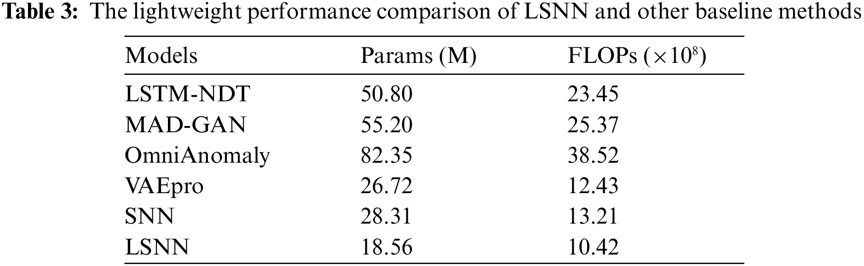
In Table 3, the proposed LSNN algorithm exhibits significantly fewer parameters and FLOPs compared to the LSTM-NDT algorithm, the MAD-GAN algorithm, the OmniAnomaly algorithm, the VAEpro algorithm and the SNN algorithm. Additionally, the proposed LSNN algorithm effectively has the better lightweight performance. On the Params metric, the proposed LSNN algorithm gains an advance about 173.7% of the LSTM-NDT algorithm, an advance about 197.4% of the MAD-GAN algorithm, an advance about 343.7% of the OmniAnomaly algorithm, an advance about 43.9% of the VAEpro algorithm and an advance about 52.5% of the SNN algorithm. On the FLOPs metric, the proposed LSNN algorithm gains an advance about 125.1% of the LSTM-NDT, an advance about 143.5% of the MAD-GAN algorithm, an advance about 269% of the OmniAnomaly algorithm, an advance about 19.3% of the VAEpro algorithm and an advance about 26.78% of the SNN algorithm.

4.4.3 Ablation Analysis in LSNN

To assess the impact of the modified Izhikevich neurons model compared to the traditional Leaky Integrate and Fire (LIF) neurons model within the lightweight edge-side fault diagnosis system (LSNN), we conducted ablation experiments. These experiments aimed to delineate performance differences between the two neurons models in managing complex network fault diagnosis tasks, with a particular focus on model accuracy. Through comparative analysis, we gained a deeper understanding of the advantages of the Izhikevich neurons model and its contribution to enhancing system performance in the SMD and ASD datasets, as detailed in Table 4.

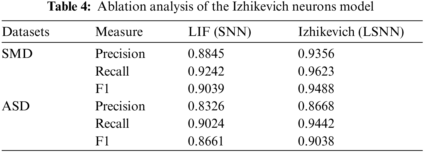
The table data indicates that for the SMD dataset, the Izhikevich neurons model generally outperforms the LIF neurons model. Precision has increased by approximately 5.78%, Recall by about 4.12%, and the F1 score by roughly 4.96%. In the ASD dataset, Precision has improved by approximately 4.11%, Recall by nearly 4.63%, and the F1 score by about 4.36%. These findings demonstrate that the Izhikevich neurons model performs better than the LIF neurons model on both datasets, making it a more effective choice for LSNN. This superior performance is likely due to the Izhikevich neurons model’s more accurate simulation of dynamic neuron behavior, which enhances its suitability for fault diagnosis tasks.

Inspired by the spiking dynamics in the basal ganglia (BG) area of the brain, we propose a pruning approach based on Fast Spiking Interneurons (FSIs) of the BG in the LSNN to enhance computational efficiency and reduce resource and energy demands. We conducted ablation experiments to compare network performance with and without this pruning method, as detailed in Table 5.

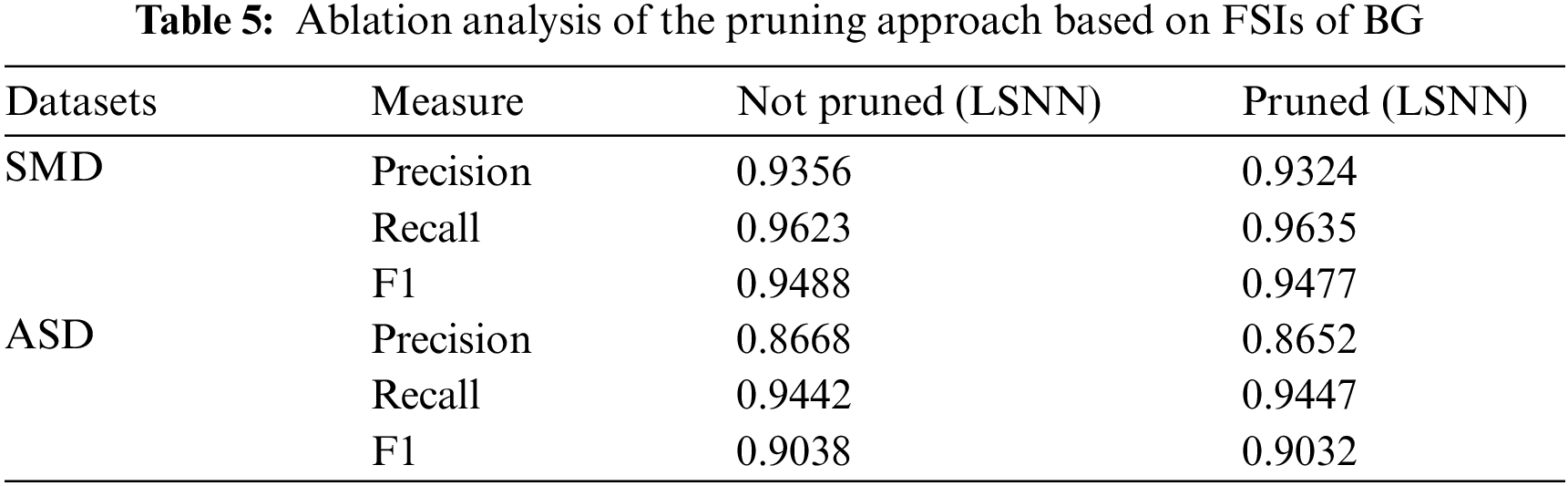
As shown in Table 5, the pruning algorithm based on Fast Spiking Interneurons (FSIs) of the basal ganglia (BG) has minimal impact on model accuracy, indicating that pruning does not significantly affect the model’s performance. Consequently, this pruning method is effective, as it reduces the model’s complexity while preserving the performance of the LSNN.

To evaluate the effectiveness of our proposed pruning method, which incorporates multiple iterative dynamic Spike Timing Dependent Plasticity (DSTDP) to optimize LSNN, we will conduct ablation experiments comparing conventional STDP with DSTDP. These experiments are designed to assess the impact of DSTDP’s dynamic features on the accuracy of fault diagnosis, as detailed in Table 6.

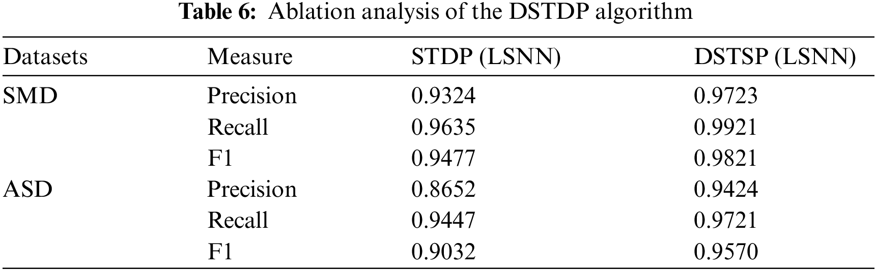
From the data presented in the table, the SMD datasets show an increase in Precision by approximately 4.28%, Recall by about 2.97%, and the F1 score by roughly 3.63%. In the ASD datasets, Precision improves by about 8.92%, Recall by approximately 2.9%, and the F1 score by around 5.96%. These results indicate noticeable improvements in both datasets when using dynamic Spike Timing Dependent Plasticity (DSTDP) compared to standard STDP. This demonstrates that the dynamic features of the DSTDP algorithm significantly enhance the network’s performance, particularly in terms of accuracy.

5  Conclusion

This paper proposes a lightweight edge-side fault diagnosis approach based on a spiking neural network (LSNN). Initially, we substitute the Leaky Integrate and Fire (LIF) neurons model with the modified Izhikevich neurons model in LSNN. The Izhikevich neurons model retains the simplicity of LIF neurons but provides more affluent behavioral properties and greater flexibility for handling diverse data inputs. Additionally, inspired by Fast Spiking Interneurons (FSIs) with high-frequency firing patterns and the spiking dynamics in the basal ganglia (BG) of the brain, we introduce a pruning approach based on FSIs of the BG to enhance computational efficiency and reduce resource and energy demands. We further develop a multiple iterative dynamic Spike Timing Dependent Plasticity (DSTDP) to enable our network to dynamically adapt and optimize its connections post-pruning, ensuring the model maintains high diagnostic accuracy despite significant reductions in complexity.

The interaction between the Izhikevich neurons and DSTDP is critical for achieving an optimal balance between lightweight architecture and diagnostic precision. This allows the LSNN to adapt to the resource limitations of edge devices while improving fault diagnosis accuracy. Our experiments on two server fault datasets demonstrate marked improvements in precision, recall, and F1 scores across three diagnostic dimensions. Moreover, lightweight metrics such as Params and FLOPs have been significantly reduced, underscoring the LSNN’s enhanced performance.

However, the performance and optimizations are based on datasets specific to network fault diagnosis, which may limit the direct applicability of our findings to other domains without further adjustments and validations. Additionally, while our model shows robustness across various fault types, future research should aim to enhance the model’s ability to handle highly imbalanced datasets, which are common in many real-world applications. Advanced data augmentation, innovative loss functions designed for imbalance, and transfer learning are potential techniques to improve model performance in such scenarios. A promising future direction for our LSNN model includes incorporating incremental learning strategies. Particularly relevant in edge computing environments, incremental learning would allow the LSNN to adapt to evolving data or scenarios without retraining from scratch, preserving previously learned knowledge while integrating new insights. This approach is crucial for sustaining the model’s relevance and effectiveness over its operational lifetime.

Acknowledgement: The authors would like to thank my supervisor Yang Yang for providing me with guidance and an experimental environment.

Funding Statement: This work is supported by National Key R&D Program of China (2019YFB2103202).

Author Contributions: The authors confirm contribution to the paper as follows: Study conception and design: Jingting Mei, Yang Yang; data collection: Yijing Lin; analysis and interpretation of results: Zhigao Peng, Lanlan Rui; draft manuscript preparation: Jingting Mei. All authors reviewed the results and approved the final version of the manuscript.

Availability of Data and Materials: The SMD and ASD databases used in this study are publicly available for research purposes. The SMD database can be requested from https://github.com/NetManAIOps/OmniAnomaly. The ASD database is available from https://github.com/zhhlee/InterFusion.

Conflicts of Interest: The authors declare that they have no conflicts of interest to report regarding the present study.

References

1. P. Bellavista, C. Giannelli, M. Mamei, M. Mendula, and M. Picone, “Application-driven network-aware digital twin management in industrial edge environments,” IEEE Trans. Ind. Inform., vol. 17, no. 11, pp. 7791–7801, 2021. doi: 10.1109/TII.2021.3067447. [Google Scholar] [CrossRef]

2. L. Wen, X. Li, L. Gao, and Y. Zhang, “A new convolutional neural network-based data-driven fault diagnosis method,” IEEE Trans. Ind. Electron., vol. 65, no. 7, pp. 5990–5998, 2017. doi: 10.1109/TIE.2017.2774777. [Google Scholar] [CrossRef]

3. E. Sisinni, A. Saifullah, S. Han, U. Jennehag, and M. Gidlund, “Industrial internet of things: Challenges, opportunities, and directions,” IEEE Trans. Ind. Inform., vol. 14, no. 11, pp. 4724–4734, 2018. doi: 10.1109/TII.2018.2852491. [Google Scholar] [CrossRef]

4. Y. Yao, S. Zhang, S. Yang, and G. Gui, “Learning attention representation with a multi-scale CNN for gear fault diagnosis under different working conditions,” Sensors, vol. 20, no. 4, pp. 1233, 2020. doi: 10.3390/s20041233. [Google Scholar] [PubMed] [CrossRef]

5. L. Zuo, L. Zhang, Z. Zhang, X. Luo, and Y. Lin, “A spiking neural network-based approach to bearing fault diagnosis,” J. Manuf. Syst., vol. 61, no. 11, pp. 714–724, 2021. doi: 10.1016/j.jmsy.2020.07.003. [Google Scholar] [CrossRef]

6. R. Kukunuri, et al., “Edgenilm: Towards nilm on edge devices,” in Proc. 7th ACM Int. Conf. Syst. Energy-Efficient Build., Cities, Transportation, 2020, pp. 90–99. [Google Scholar]

7. Y. Lei, B. Yang, X. Jiang, F. Jia, N. Li and A. K. Nandi, “Applications of machine learning to machine fault diagnosis: A review and roadmap,” Mech. Syst. Signal. Process., vol. 138, pp. 106587, 2020. doi: 10.1016/j.ymssp.2019.106587. [Google Scholar] [CrossRef]

8. D. Dou, J. Yang, J. Liu, and Y. Zhao, “A rule-based intelligent method for fault diagnosis of rotating machinery,” Knowl. Based Syst., vol. 36, no. 4, pp. 1–8, 2012. doi: 10.1016/j.knosys.2012.05.013. [Google Scholar] [CrossRef]

9. L. Ciabattoni, F. Ferracuti, A. Freddi, and A. Monteriù, “Statistical spectral analysis for fault diagnosis of rotating machines,” IEEE Trans. Ind. Electron., vol. 65, no. 5, pp. 4301–4310, 2017. doi: 10.1109/TIE.2017.2762623. [Google Scholar] [CrossRef]

10. Y. Xu, Y. Sun, J. Wan, X. Liu, and Z. Song, “Industrial big data for fault diagnosis: Taxonomy, review, and applications,” IEEE Access, vol. 5, pp. 17368–17380, 2017. doi: 10.1109/ACCESS.2017.2731945. [Google Scholar] [CrossRef]

11. W. Yu and C. Zhao, “Online fault diagnosis for industrial processes with Bayesian network-based probabilistic ensemble learning strategy,” IEEE Trans. Autom. Sci. Eng., vol. 16, no. 4, pp. 1922–1932, 2019. doi: 10.1109/TASE.2019.2915286. [Google Scholar] [CrossRef]

12. Y. Zhang, J. Ma, J. Zhang, and Z. Wang, “Fault diagnosis based on cluster analysis theory in wide area backup protection system,” in 2009 Asia-Pac. Power and Energy Eng. Conf., Wuhan, China, 2009, pp. 1–4. [Google Scholar]

13. J. Liu, et al., “Data-driven and association rule mining-based fault diagnosis and action mechanism analysis for building chillers,” Energy Build., vol. 216, pp. 109957, 2020. doi: 10.1016/j.enbuild.2020.109957. [Google Scholar] [CrossRef]

14. Z. Yin and J. Hou, “Recent advances on SVM based fault diagnosis and process monitoring in complicated industrial processes,” Neurocomputing, vol. 174, no. 6, pp. 643–650, 2016. doi: 10.1016/j.neucom.2015.09.081. [Google Scholar] [CrossRef]

15. Y. Lecun, Y. Bengio, and G. Hinton, “Deep learning,” Nature, vol. 521, no. 7553, pp. 436–444, 2015. [Google Scholar] [PubMed]

16. X. Wen and Z. Xu, “Wind turbine fault diagnosis based on ReliefF-PCA and DNN,” Expert. Syst. Appl., vol. 178, no. 11, pp. 115016, 2021. doi: 10.1016/j.eswa.2021.115016. [Google Scholar] [CrossRef]

17. P. Yao, S. Yang, and P. Li, “Fault diagnosis based on RseNet-LSTM for industrial process,” in 2021 IEEE 5th Adv. Inf. Technol., Electronic Automation Control Conf. (IAEAC), Chongqing, China, 2021, pp. 728–732. [Google Scholar]

18. H. Liu, J. Zhou, Y. Zheng, W. Jiang, and Y. Zhang, “Fault diagnosis of rolling bearings with recurrent neural network-based autoencoders,” ISA Trans., vol. 77, pp. 167–178, 2018. doi: 10.1016/j.isatra.2018.04.005. [Google Scholar] [PubMed] [CrossRef]

19. S. Zhong, S. Fu, and L. Lin, “A novel gas turbine fault diagnosis method based on transfer learning with CNN,” Measurement, vol. 137, no. 5, pp. 435–453, 2019. doi: 10.1016/j.measurement.2019.01.022. [Google Scholar] [CrossRef]

20. K. Zhang, J. Chen, S. He, F. Li, Y. Feng and Z. Zhou, “Triplet metric driven multi-head GNN augmented with decoupling adversarial learning for intelligent fault diagnosis of machines under varying working condition,” J. Manuf. Syst., vol. 62, pp. 1–16, 2022. doi: 10.1016/j.jmsy.2021.10.014. [Google Scholar] [CrossRef]

21. H. Pan, X. He, S. Tang, and F. Meng, “An improved bearing fault diagnosis method using one-dimensional CNN and LSTM,” J. Mech. Eng., vol. 64, no. 7, pp. 443–452, 2018. [Google Scholar]

22. D. Chen, R. Liu, Q. Hu, and S. X. Ding, “Interaction-aware graph neural networks for fault diagnosis of complex industrial processes,” IEEE Trans. Neural Netw. Learn. Syst., vol. 34, no. 9, pp. 6015–6028, 2021. doi: 10.1109/TNNLS.2021.3132376. [Google Scholar] [PubMed] [CrossRef]

23. S. Rothe, S. Narayan, and A. Severyn, “Leveraging pre-trained checkpoints for sequence generation tasks,” Trans. Assoc. Comput. Linguist., vol. 8, pp. 264–280, 2020. doi: 10.1162/tacl_a_00313. [Google Scholar] [CrossRef]

24. M. Reid, E. Marrese-Taylor, and Y. Matsuo, “Subformer: Exploring weight sharing for parameter efficiency in generative transformers,” arXiv preprint arXiv:2101.00234, 2021. [Google Scholar]

25. S. Takase and S. Kiyono, “Lessons on parameter sharing across layers in transformers,” arXiv preprint arXiv:2104.06022, 2021. [Google Scholar]

26. M. S. Zhang and B. C. Stadie, “One-shot pruning of recurrent neural networks by Jacobian spectrum evaluation,” arXiv preprint arXiv:1912.00120, 2020. [Google Scholar]

27. Y. Wang, L. Wang, V. O. K. Li, and Z. Tu, “On the sparsity of neural machine translation models,” arXiv preprint arXiv:2010.02646, 2010. [Google Scholar]

28. D. Guo, A. M. Rush, and Y. Kim, “Parameter-efficient transfer learning with diff pruning,” arXiv preprint arXiv:2012.07463, 2020. [Google Scholar]

29. F. Lagunas, E. Charlaix, V. Sanh, and A. M. Rush, “Block pruning for faster transformers,” arXiv preprint arXiv:2109.04838, 2021. [Google Scholar]

30. M. Xia, Z. Zhong, and D. Chen, “Structured pruning learns compact and accurate models,” arXiv preprint arXiv:2204.00408, 2022. [Google Scholar]

31. V. A. Demin, et al., “Necessary conditions for STDP-based pattern recognition learning in a memristive spiking neural network,” Neural Netw., vol. 134, pp. 64–75, 2021. doi: 10.1016/j.neunet.2020.11.005. [Google Scholar] [PubMed] [CrossRef]

32. Y. Hao, X. Huang, M. Dong, and B. Xu, “A biologically plausible supervised learning method for spiking neural networks using the symmetric STDP rule,” Neural Netw., vol. 121, no. 10, pp. 387–395, 2020. doi: 10.1016/j.neunet.2019.09.007. [Google Scholar] [PubMed] [CrossRef]

33. G. Kim, K. Kim, S. Choi, H. J. Jang, and S. O. Jung, “Area-and energy-efficient STDP learning algorithm for spiking neural network SoC,” IEEE Access, vol. 8, pp. 216922–216932, 2020. doi: 10.1109/ACCESS.2020.3041946. [Google Scholar] [CrossRef]

34. D. Tal and E. L. Schwartz, “Computing with the leaky integrate-and-fire neuron: Logarithmic computation and multiplication,” Neural Comput., vol. 9, no. 5, pp. 305–318, 1997. doi: 10.1162/neco.1997.9.2.305. [Google Scholar] [PubMed] [CrossRef]

35. E. M. Izhikevich, “Simple model of spiking neurons,” IEEE Trans. Neural Netw., vol. 14, no. 6, pp. 1569–1572, 2003. doi: 10.1109/TNN.2003.820440. [Google Scholar] [PubMed] [CrossRef]

36. A. L. Hodgkin and A. F. Huxley, “A quantitative description of membrane current and its application to conduction and excitation in nerve,” J. Physiol., vol. 117, no. 5, pp. 500–544, 1952. doi: 10.1113/jphysiol.1952.sp004764. [Google Scholar] [PubMed] [CrossRef]

37. Y. Yu and Q. Wang, “Oscillation dynamics in an extended model of thalamic-basal ganglia,” Nonlinear Dyn., vol. 98, no. 2, pp. 1065–1080, 2019. doi: 10.1007/s11071-019-05249-2. [Google Scholar] [CrossRef]

38. A. C. Bostan and P. L. Strick, “The basal ganglia and the cerebellum: Nodes in an integrated network,” Nat. Rev. Neurosci., vol. 19, no. 6, pp. 338–350, 2018. doi: 10.1038/s41583-018-0002-7. [Google Scholar] [PubMed] [CrossRef]

39. T. Masquelier, R. Guyonneau, and S. J. Thorpe, “Competitive STDP-based spike pattern learning,” Neural Comput., vol. 21, no. 5, pp. 1259–1276, 2009. doi: 10.1162/neco.2008.06-08-804. [Google Scholar] [PubMed] [CrossRef]

40. Y. Su, Y. Zhao, C. Niu, R. Liu, W. Sun and D. Pei, “Robust anomaly detection for multivariate time series through stochastic recurrent neural network,” in Proc. 25th ACM SIGKDD Int. Conf. Knowl. Discov.Data Min., New York, NY, USA, 2019, pp. 2828–2837. [Google Scholar]

41. Z. Li et al., “Multivariate time series anomaly detection and interpretation using hierarchical inter-metric and temporal embedding,” in Proc. 27th ACM SIGKDD Conf. Knowl. Discov. Data Min., New York, NY, USA, 2021, pp. 3220–3230. [Google Scholar]

42. A. Abdulaal, Z. Liu, and T. Lancewicki, “Practical approach to asynchronous multivariate time series anomaly detection and localization,” in Proc. 27th ACM SIGKDD Conf. Knowl. Discov. Data Min., New York, NY, USA, 2021, pp. 2485–2494. [Google Scholar]

43. D. Li, D. Chen, B. Jin, L. Shi, J. Goh, and S. K. Ng, “MAD-GAN: Multivariate anomaly detection for time series data with generative adversarial networks,” in Int. Conference Artif. Neural Netw., Munich, Germany, 2019, pp. 703–716. [Google Scholar]

44. Y. Ikeda, K. Tajiri, Y. Nakano, K. Watanabe, and K. Ishibashi, “Estimation of dimensions contributing to detected anomalies with variational autoencoders,” arXiv preprint arXiv:1811.04576, 2018. [Google Scholar]