Deep Learning-Based ECG Classification for Arterial Fibrillation Detection

1  Introduction

The prevalence of cardiovascular illnesses has been increasing in contemporary society, affecting not only older individuals but also younger populations because of their primarily inactive way of life. Atrial fibrillation is a prevalent cardiac disorder often seen in adults, characterized by anomalous electrical impulses within the heart’s atria. This cardiac arrhythmia is often seen and is distinguished by atypical, irregular, and frequently accelerated cardiac contractions. Could be paraphrased as Atrial Fibrillation (AFib) is associated with significant morbidity and mortality, particularly when not promptly managed. This condition has been associated with an elevated likelihood of experiencing significant cardiac consequences, including heart failure, thromboembolic events, and cerebrovascular accidents [1].

Based on data provided by the World Health Organization (WHO), it is anticipated that AFib impacts around 33.5 million individuals globally. Furthermore, the incidence of this condition is projected to rise because of population aging and the escalating rates of obesity and diabetes among younger individuals [2]. In AFib cases, blood pooling in the atria may occur, potentially leading to the formation of blood clots. These clots can induce heart failure or migrate to the cerebral region, posing a risk to the brain. Suppose a blood clot migrates to the cerebral region. In that case, it can potentially induce a cerebrovascular accident, often referred to as a stroke, which typically has a high mortality rate. AFib is a prominent risk factor for stroke since those diagnosed with AFib have a much higher likelihood of experiencing a stroke compared to those without this condition [3]. During an episode of AFib, the cardiac rhythm becomes erratic, resulting in an aberrant heart rate. Electrocardiogram (ECG) monitoring is a diagnostic technique that is both non-invasive and readily accessible. It can identify AFib and other irregular heart rhythms, enabling prompt management and improving patient outcomes [4].

The analysis of vast ECG signal data poses challenges for medical professionals, given its complexity and the need to process substantial information. The presence of noise and abnormalities in ECG readings poses a significant challenge to human observers’ reliable identification of AFib. Nevertheless, deep learning algorithms can analyse ECG data and acquire knowledge of patterns linked to AFib, enabling enhanced precision and efficiency in identification. Moreover, it is possible to train deep learning algorithms using extensive datasets of ECG signals, enabling them to acquire knowledge from a wide array of data and enhance their precision as time progresses [5]. Therefore, the use of deep learning models has the potential to enhance the dependability and uniformity of AFib diagnosis, therefore playing a crucial role in enhancing patient outcomes and mitigating the likelihood of problems.

Designing a precise algorithm capable of effectively discerning AFib with a notable level of accuracy and a minimal occurrence of false alarms while avoiding misclassification of AFib as other arrhythmic disorders is a considerable challenge. The exact timing of an AFib episode experienced by a patient is of utmost importance in precisely capturing the event via ECG signals [6]. Deep learning algorithms often encounter challenges in accurately detecting AFib due to arrhythmias with similar features, such as repeated premature atrial contractions. The primary contribution of this work is in the design and development of a deep learning model that exhibits a high level of accuracy and precision in predicting AFib while also demonstrating efficient computing performance. Various deep learning models are analysed concerning metrics such as accuracy, precision, and computational time. The selection of the best-fit model is based on its ability to achieve optimal accuracy in identifying AFib while minimizing the occurrence of erroneous diagnoses.

The detection of Atrial Fibrillation (AFib) through Electrocardiogram (ECG) signals is a critical step in preventing severe cardiac events and enhancing patient recovery. However, the application of deep learning techniques to accurately identify AFib faces challenges such as overfitting and inconsistent performance across various datasets. These issues underline the need for robust, reliable deep learning models that can adapt to the complexities of ECG data to improve diagnostic accuracy and patient outcomes.

There is a gap in the comprehensive comparison of deep learning architectures for AFib detection. Particularly, studies comparing the performance of advanced models like ResNet-50 and DenseNet-121 in processing ECG signals are limited. This gap indicates a need for systematic evaluations that can guide the selection of optimal architectures for specific clinical applications. Another significant gap lies in addressing the consistency of model accuracy across different datasets. Many existing studies fail to thoroughly investigate or mitigate the variations in model performance when applied to diverse ECG datasets. This inconsistency poses a barrier to the deployment of deep learning solutions in a real-world clinical setting, where data variability is a common challenge.

In this paper contribution are following:

•   Showcased ResNet-50’s Superiority: Proved through rigorous evaluation that ResNet-50 outperforms DenseNet-121 in detecting AFib from ECG signals, based on metrics such as accuracy, precision, and sensitivity.

•   Advanced Methodological Evaluation: Employed a comprehensive set of metrics, including loss, accuracy, precision, sensitivity, and Area Under the Curve (AUC), to assess the performance of deep learning models in AFib detection.

•   Addressed the Need for Robust Detection: Highlighted the effectiveness of ResNet-50 in offering a more consistent and accurate method for AFib detection, for its application in clinical settings.

•   Contributed to Research Foundation: The findings provide a solid foundation for future research to build more efficient and accurate deep learning models for ECG-based AFib detection, addressing critical gaps in the literature and clinical practice.

2  Related Works

The topic of atrial fibrillation has been extensively investigated in prior research. A one-dimensional Convolutional Neural Network (CNN)-based real-time ECG categorization system was shown. Each patient’s individual demands have been considered when designing the system. Kiranyaz et al. [7] used 1-Dimensional Convolutional Neural Networks (1-D CNN) has resulted in a success rate of 98.3%. In their work, the authors introduced a unique method that used a wavelet-based method for ECG delineation with the express goal of diagnosing AFib. A 96.8% accuracy rate was discovered after completing validations to identify AFib using the described technique [8]. The automatic identification of ventricular fibrillation was made possible with the introduction of a deep learning-based method. To improve the quality of the ECG data, wavelet processing and sliding window filtering techniques were created. A technique has been created to recognize R waves that exhibit competence. According to the research results, the algorithm designed to detect atrial fibrillation has an accuracy rate of 84.0%, a sensitivity rate of 84.26%, and a specificity rate of 93.23% [9].

The objective is to assess and compare the suggested methods for atrial fibrillation detection. The research findings indicated a high validation accuracy of 0.8765 when using the final technique [10], which incorporated a Convolutional Long Short-Term Memory (CLSTM) model for categorizing P wave detection. Convolutional layers and Long Short-Term Memory (LSTM) are both a part of the present structure. Another method involves gathering ground truth data by personally examining the model’s output [11]. This data is used to compare the frequency of true positive and true negative predictions about the patients’ mobile settings. the development of a deep-learning classification scheme for cardiac arrhythmias, including atrial fibrillation. The study employed a CNN model that was trained on a significant dataset of 91,232 single-lead ECG recordings from 53,549 patients. The CNN model’s 34 layers were utilized in its development. The model’s excellent effectiveness in detecting atrial fibrillation is shown by the Area Under the Receiver Operating Characteristic Curve (AUC-ROC) value of 0. 97. The results of the study show that deep learning models can accurately diagnose and categorize arrhythmias with the same efficacy as skilled human cardiologists [12]. The use of deep CNN for the identification of AFib in ECG data was examined in the study by Xia et al. [13]. The researchers came up with a two-stage process, where they first employed a shallow CNN to extract essential details from ECG segments. Based on the examination of 25 two-channel ECG recordings taken from the Physio Net MIT-BIH Atrial Fibrillation Database, the researchers in this study developed and validated a model. The method used in this study, which makes use of deep learning techniques, has proven to be remarkably effective at spotting atrial fibrillation. According to the data reported Xia et al. [13], there is 98.4% sensitivity and 96.3% specificity. Based on concise single-lead ECG data, a deep learning approach was presented that employed 1D-CNN to categorize AFib. The model’s improved F1-score indicated that it performed at a better level than traditional machine learning techniques [14]. The researchers used the dataset provided by the 2017 PhysioNet/CinC Challenge for their analysis. The study’s authors have established a standard for future research efforts by comprehensively analyzing the strengths and weaknesses of different approaches [15]. Development of an extensive deep-learning framework that utilizes CNNs and bidirectional LSTM to identify AFib in single-lead ECG data. The research presented in the study showcased positive results and indicated the possibility of detecting AFib in real-time using wearable technology [16]. A deep-learning methodology to identify AFib was introduced by using morphological and rhythm data derived from ECG recordings. The study presented evidence of the effectiveness of using a combination of traits in identifying AFib, as the proposed strategy showed superior performance compared to competing approaches [17]. Data obtained from a single-lead ECG to construct a deep-learning model to conduct AFib screening. The researchers used a rigorous approach to accurately detect AFib in a particular population, demonstrating a sensitivity of 95.6% and a specificity of 97.5% [18].

The identification of atrial fibrillation in two-dimensional ECG was suggested. The methodology employed in their research, which showcased the potential advantages of employing two-dimensional representations for deep learning-based identification of AFib [19], entailed transforming one-dimensional ECG data into two-dimensional images. This approach yielded notable levels of precision in the detection of AFib.

One limitation of the literature review studied, as represented in Table 1 and shows that it relies on the assumption that the P wave is the most reliable fiducial point for detecting atrial fibrillation. While this may be true in many cases, there may be patients with other ECG features more indicative of atrial fibrillation. Additionally, the model is only trained on P waves, which may limit its ability to detect other important ECG features. Another area for improvement is that the model’s performance is only validated on a feed-forward neural network, which may not represent the performance on other types of neural networks. Valuing the model’s performance on various network architectures would be beneficial to ensure its effectiveness.

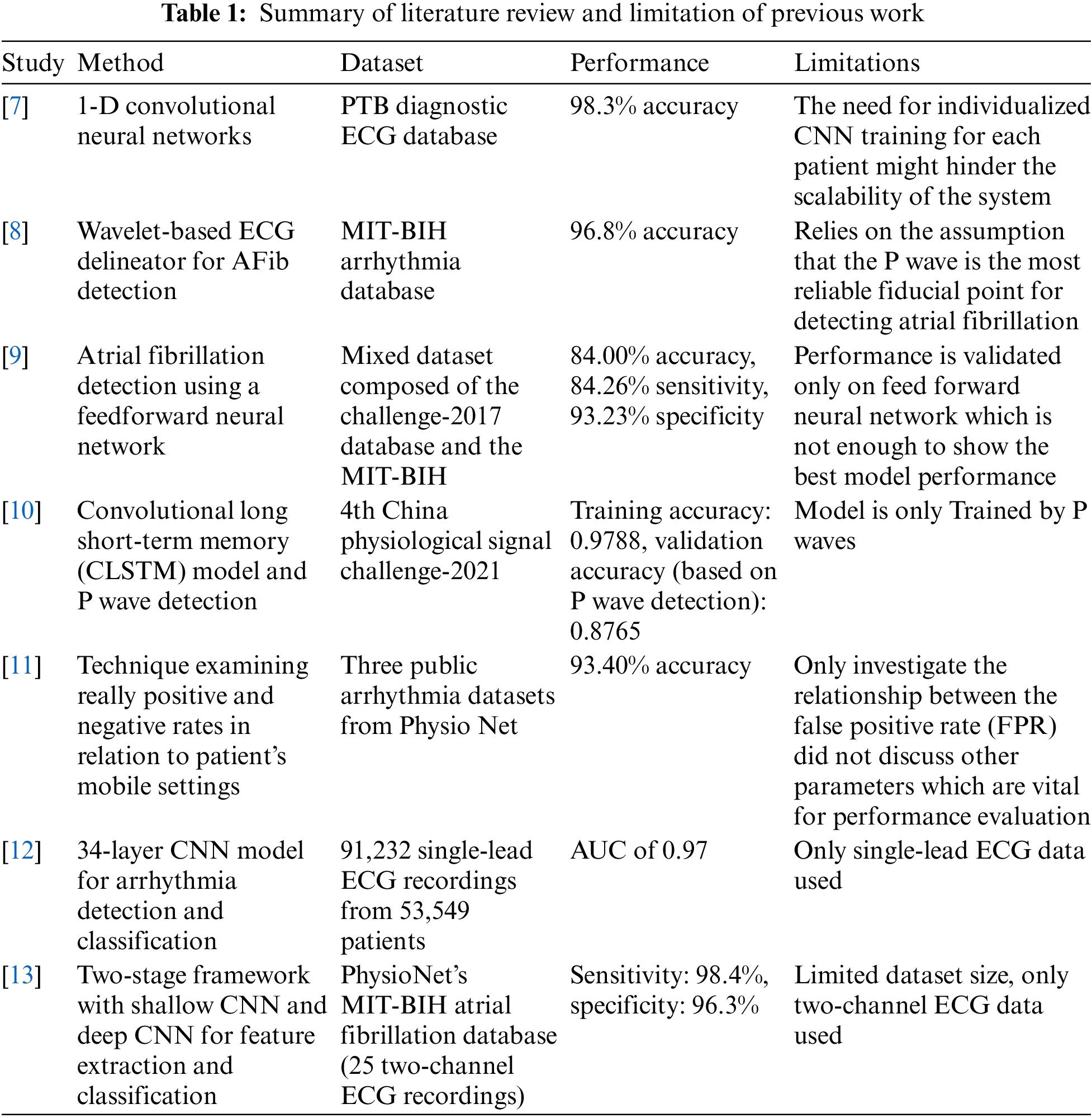
Furthermore, the model only investigates the relationship between the False Positive Rates (FPR), which may not comprehensively assess the model’s performance. Evaluating other performance metrics such as sensitivity, specificity, and accuracy would be helpful. Finally, the dataset size used in the study is limited to only two-channel ECG data, which may need to be increased for training a robust and accurate model for detecting atrial fibrillation. It would be beneficial to train the model on larger datasets with more channels to improve its accuracy and generalizability.

3  Methodology

In this study, CNN is used for the classification of ECG arrhythmia. The methodology is divided into sections such as follows: a) Data Set b) Data Pre-processing c) Data Engineering d) ResNet-50 and DenseNet-121.

3.1 Data Set

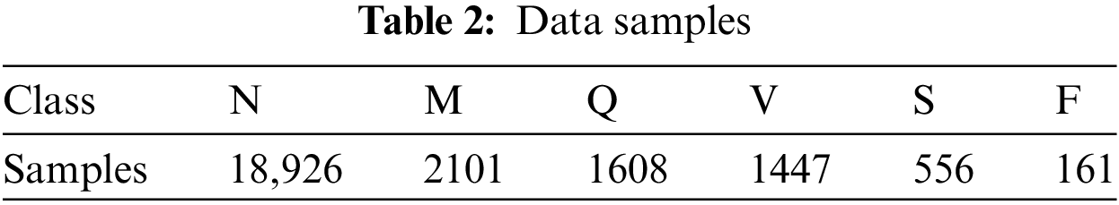
Heartbeat signals from the MIT-BIH Arrhythmia Dataset and the PTB Diagnostic ECG Database were combined to create the dataset for this investigation [20]. To train deep neural networks for the categorization of heartbeats, this dataset provides sufficient instances. Researchers have looked at deep neural network architectures and transfer learning’s capacity to classify ECG heartbeats as either normal or affected by various arrhythmias and myocardial infarction. The dataset consists of 109,446 samples in total, which are divided into the following five groups: N, S, V, F, and Q. The MIT-BIH dataset is the source of these samples.

The dataset also includes 14,552 samples from the PTB Diagnostic Database that have been divided into two categories. For both datasets, the sampling rate is set at 125 Hz. Preprocessing, segmentation, and image conversion were applied to the ECG arrhythmias. The dataset has been divided into training and validation halves, with 80% of the samples going to training and 20% going to validation.

Table 2 shows the number of samples of each class in the data set.

Combining heartbeat signals from the MIT-BIH Arrhythmia Dataset and the PTB Diagnostic ECG Database significantly enhances the dataset’s diversity, essential for developing robust deep learning models for ECG signal classification. The integration of these datasets introduces a broader spectrum of ECG patterns, encompassing various arrhythmias and myocardial infarction types across different patient demographics. This diversity aids in improving the models’ generalization ability, reducing the risk of overfitting to specific dataset characteristics, and ensuring the models learn to identify genuine underlying patterns indicative of cardiac conditions. Moreover, the merger results in a larger dataset size, offering 109,446 and 14,552 samples from each dataset respectively, which is beneficial for deep learning as it provides more examples for the model to learn from, leading to better performance and reliability.

The methodology for combining the datasets involves preprocessing and segmentation to normalize and ensure consistency between the datasets, including filtering, noise reduction, and signal amplitude normalization. ECG signals were then segmented into individual heartbeats or fixed-length segments, suitable for analysis. Additionally, the data was converted into a format conducive to deep learning, potentially using image conversion techniques to transform time-series data into spectrogram or waveform images, facilitating the use of convolutional neural networks. Both datasets shared a sampling rate of 125 Hz, maintaining consistency in temporal resolution across the combined dataset. Finally, the dataset was randomly divided into training and validation subsets, allocating 80% for training to maximize learning opportunities and 20% for validation to assess the model’s performance and its ability to generalize across unseen data. This meticulous process of combining datasets underpins the development of more accurate, reliable, and generalizable models for detecting cardiac conditions through ECG signals [21].

3.2 Data Pre-Processing

In the dataset preprocessing phase, critical steps are undertaken to ensure the ECG signal data is optimally prepared for input into deep learning models, focusing on normalization, noise removal, and amplitude scaling. The aim is to standardize the data to achieve uniformity in value ranges across different sensors and leads, enhancing the model’s ability to learn and identify patterns indicative of arrhythmias.

Normalization is a pivotal preprocessing step where each ECG signal lead’s data is scaled to ensure that all values lie within a standardized range, facilitating faster and more efficient model convergence. This is achieved using the formula.

X=(X−x_min)(x_max−x_min)(1)

where x_min an x_max represent the minimum and maximum amplitude values within a lead, respectively. As a result, the processed signals have amplitudes normalized to a range greater than 0 and less than 1, making the data consistent and easier for the model to process.

To address the issue of noise, which can significantly affect the accuracy of ECG signal interpretation, a Gaussian filter is applied. This method is chosen for its proficiency in reducing Gaussian noise—common in ECG recordings—while preserving essential signal features. The inclusion of Gaussian noise into the signal mimics real-world signal disturbances, providing a realistic scenario for the model to learn from. Furthermore, amplitude scaling is employed to reflect real variations in signal strength, adjusting the ECG signal’s amplitude by a factor to simulate these fluctuations authentically. Additionally, to simulate baseline drifts often seen in ECG data, a random shift in the signal’s baseline is introduced.

After these preprocessing steps, the dataset is divided into training and validation subsets. The training set is used to teach the convolutional neural network (CNN) model, allowing it to learn and adapt to the characteristics of ECG signals. In contrast, the validation set serves to evaluate the model’s performance and guide the adjustment of its hyperparameters. This thorough preparation of the ECG data is essential for developing a model capable of accurately classifying arrhythmias, ensuring that it is trained and validated on data that closely resembles the conditions encountered in clinical environments.

3.3 Data Engineering

By using CNN, it is possible to categorize ECG data into arrhythmia and normal categories. The CNN model is a well-known deep learning strategy that has been shown to be very effective in several medical fields, particularly in arrhythmia identification. Following the use of pre-processing methods, the dataset is divided into several subsets for the purposes of training and validation. While the training set is used to train the CNN model, the validation set is used to pick a model and tune its hyperparameters. Multiple convolutional layers, max-pooling layers, and finally fully linked layers make up the architecture of a CNN. By examining the characteristics noticed by the convolutional layers, fully connected layers are used to identify the input ECG data [22].

The categorical cross-entropy loss function and the Adam optimizer are used in the training method to improve the performance of the CNN model. The model’s training phase is carried out across several epochs with a batch size of 32. A popular strategy is to use a learning rate that is initially set at 0.001 and then progressively dropped over the course of the learning process to reduce the possible problem of overfitting. Following the training process, the effectiveness of the CNN model is assessed using several measures, including accuracy, precision, sensitivity, and F1-score. The confusion matrix shows that the model distinguishes between arrhythmia signals and normal signals with a high degree of accuracy and few instances of misclassification.

Fig. 1 provides a thorough representation of the intended system. The system consists of a dataset that undergoes initial preprocessing. Subsequently, the preprocessed dataset is divided into subsets during the data splitting phase. These subsets are then utilized in the prediction model, which constitutes the processing phase of the system. The accuracy of classification outcomes is assessed by comparing them to the expected outcomes. If the desired outcomes are obtained and the model is saved in the cloud, the classification results are considered satisfactory. Otherwise, the model is sent back to the training phase for further refinement. The models are subsequently imported from the cloud, and predictions are generated using the validation data. Classifications results are displayed at the end which shows that the person is arrhythmic or not [23].

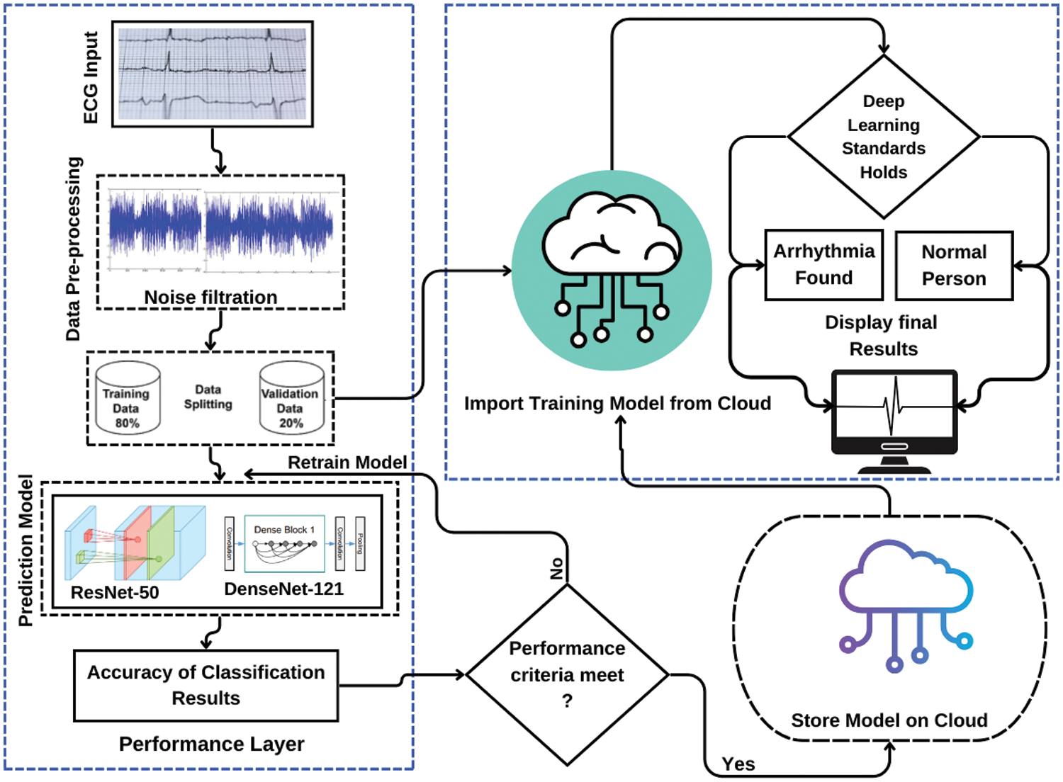
Figure 1: Complete system overview diagram

For data pre-processing Google Compute Engine backend (GPU) is used where data set is trained and validated using ResNet-50 and DenseNet-121 based on DCNN architectures. Firstly, data set is divided in two sets, i.e., training data set and validation data set. The training data set consists of 80% while validation data set comprises of about 20%.

3.4 ResNet-50 and DenseNet-121

The classification of arrhythmia employs two contemporary convolutional neural network architectures, namely ResNet-50 and DenseNet-121. Object recognition is a prevalent task in computer vision that can be effectively accomplished through the utilization of ResNet-50’s convolutional neural network architecture. In recent years, the technique of ECG signal analysis has been utilized for the purpose of identifying and categorizing arrhythmia, resulting in significant benefits. ResNet-50 is the superior deep neural network architecture in terms of accuracy and training time when compared to other CNN models. The research utilizes ResNet-50 modelling. Skip connections are utilized to facilitate the training of neural networks with significant depth. A ResNet-50 residual block comprises of a batch normalization layer, two convolutional layers, and a Rectified Linear Unit (ReLU) activation function. The residual block’s output is augmented by the input via a shortcut connection that bypasses the convolutional layers. The residual block generates an output that is the result of an element-wise addition operation between the input and the residual, resulting in their summation (i.e., the difference between the input and output of the convolutional layers). The ResNet-50 architecture is characterized by an increasing quantity of residual blocks, with each layer of the network featuring one such block. The process of feature extraction commences with the utilization of a convolutional layer in the network, which employs a sequence of filters to the input ECG signal. After the convolutional layer, a batch normalization layer is employed to standardize the output of the former, thereby reducing the covariate shift that may occur within the neural network. Subsequently, a ReLU activation function is employed to introduce nonlinearity to the output. The residual block comprises of two convolutional layers, batch normalization, and ReLU activation. The output of the residual block is then fed back into the network after the first layer. The final layer of a fully interconnected network is responsible for producing the output classification [24].

Represent the output of each Convolutional Layer as follows shown in Eq. (2).

Y=f(w.x+b)(2)

The output of each Residual Block is then concatenated with the input tensor and passed to the next block shown in Eq. (3).

Z=f(W2.f(W1.X+b1)+b2+X)(3)

Represent the global average pooling operation as shown in Eq. (4).

V=1H∗W∗sum(Z)(4)

The output of the fully connected layer is then passed through a SoftMax function to obtain a probability distribution over the classes as shown in Eq. (5).

P=softmax(W.V+b)(5)

The convolutional layer in our model produced Eq. (1). W refers for the weight’s matrix, X is the input tensor, b stands for the bias term, and f stands for the activation function applied elementwise to the input tensor. Y is the resultant output tensor. To extract spatial characteristics and patterns from the input data, the convolutional layer applies a number of filters to the data. In Eq. (2), residual blocks are used to enhance the model’s learning capacity after the convolutional layers. X is the input tensor, W1 and W2 stand for the weight matrices, b1 and b2 for the bias terms, and f for the activation function. These residual blocks mitigate the vanishing gradient issue and enable the direct flow of gradients across the network, enhancing the model’s ability to learn complicated features. A global average pooling technique is used in Eq. (3) after the remaining blocks. V is the result, Z is the input tensor from the preceding layer, and H and W are the feature maps’ respective height and breadth. The global average pooling technique shrinks the feature maps’ spatial dimensions, condensing the data while lowering computational complexity and overfitting risk. To produce a probability distribution across the classes, the output of the global average pooling is then sent via a fully connected layer and a SoftMax function in step Eq. (4). W stands for the weight’s matrix, V for the global average pooling layer output, and b for the bias term. The SoftMax function makes sure that all class probabilities add up to one, giving the model’s output a coherent interpretation. Together, these equations describe the network’s forward pass, which enables it to efficiently learn hierarchical features and categorize incoming samples. Convolutional layers, residual blocks, global average pooling, and a fully connected layer with a SoftMax function make up the model’s architecture, which supports effective feature extraction and reliable input data categorization.

When compared to other CNN designs, convolutional neural networks, like DenseNet-121, are renowned for their high accuracy and efficient parameter use. The building’s framework is made of substantial blocks with several, intricately interwoven layers. Because of the network’s extensive connectedness, it may quickly acquire complicated characteristics by using learnt features at each layer. The final output of the network is generated by sending the outputs of all dense blocks through a fully connected layer and summing them together. The input of the DenseNet-121 architecture is a pre-processed 12-lead ECG signal. The input signal undergoes a convolutional process using a 7 × 7 kernel and 64 filters. Subsequently, a ReLU-based activation function and a batch normalization layer are employed. The output of the initial convolutional layer is subjected to a compact arrangement of six convolutional layers, with each layer comprising 32 filters. After the compact block, a transition layer is employed, which comprises of a 1 × 1 convolutional layer and average pooling, with the purpose of reducing the spatial dimensions of the resultant feature maps. Subsequently, the output of the layer is passed through an additional transition layer and a dense block. The final dense block comprises 23 convolutional layers, with each layer consisting of 32 filters. Following the combination of the output of each dense block with the output of the remaining blocks, the resultant output is subjected to global average pooling, where it is averaged. The final classification is obtained by utilizing a fully connected layer that employs a SoftMax activation function to process the output of the global average pooling layer [25].

The dataset that has undergone pre-processing and enhancement is utilized for the training of the DenseNet-121 architecture. The Adam optimization algorithm is employed for the purpose of training, utilizing a batch size of 64 and a learning rate of 0.001. To mitigate the issue of overfitting, the model’s training process is concluded prematurely after multiple epochs. The monitoring of the model’s advancement during training can be accomplished by utilizing the validation set, while the evaluation of the outcome can be conducted by means of the validation set. The evaluation of the model is based on several metrics, including accuracy, precision, sensitivity, F1-score, and area under the receiver operating characteristic curve [26].

The output of each Dense Block is then concatenated with the input tensor and passed to the next block shown in Eq. (6).

Z=concat(X,Y)(6)

As the output of each Dense Block is concatenated with the input tensor and passed to the next block as shown in Eq. (5): Z = concat (X, Y). The concatenation operation used here is typically along the feature axis (also known as the channel axis). This operation retains the spatial dimensions (height and width) of the input and output tensors while increasing the number of channels (features) [27].

For our investigation into ECG signal classification using DenseNet-121 and ResNet-50, the models were deployed within the TensorFlow and Keras frameworks, chosen for their comprehensive support for convolutional neural networks. The training was conducted over 50 epochs, incorporating the Adam optimizer and categorical cross-entropy as the loss function, to best suit the multiclass classification challenge presented by our dataset. Aware of the potential for overfitting, an early stopping mechanism was employed, designed to halt the training if the validation loss failed to improve over a span of 5 consecutive epochs. This precaution was essential for maintaining the models’ generalization capabilities over unseen data [28,29].

Addressing the issue of class imbalance—a common challenge in medical datasets where certain conditions are significantly more prevalent than others—was crucial for ensuring equitable model sensitivity across all arrhythmia categories. To this end, class weights were adjusted during the training phase, thereby amplifying the importance of underrepresented classes in the dataset. Furthermore, data augmentation techniques were applied to enhance the dataset’s diversity, effectively enriching the models’ training environment. The progress of both models was closely monitored through the analysis of training and validation curves, enabling the timely identification and correction of overfitting or underfitting, thus assuring a balanced and effective learning process for both DenseNet-121 and ResNet-50 in their task of ECG signal classification [30–32].

4  Results and Discussion

The results of ResNet-50, DenseNet-121 based on DCNN architectures are evaluated based on classification performance metric, validation Loss, validation Accuracy, validation Precision, validation Sensitivity, and validation AUC and all of them are for training set as well of a complete model.

4.1 ResNet-50

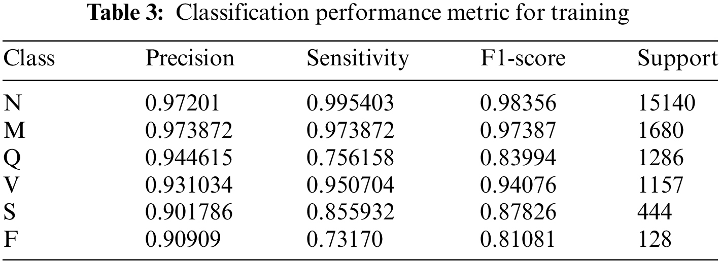
The performance of the ResNet-50 models in a multi-class classification task that includes six unique classes, namely F, M, N, Q, S, and V, is valuably revealed by the evaluation metrics given in this work. Analyzing the accuracy, sensitivity, F1-score, and support measures for each class will allow us to assess the model’s performance in detail.

An accuracy of 0.97, sensitivity of 0.99, and F1-score of 0.98 were shown by the model for class N (supported by 15,140 examples), indicating remarkable detection and classification skills. The performance of Class M was excellent, with accuracy, sensitivity, and F1-score all coming in at 0.97 over 1680 cases.

With 1286 examples, Class Q showed accuracy of 0.94, sensitivity of 0.76, and an F1-score of 0.84, suggesting some memory inconsistencies. A balanced performance was shown by Class V, which had 1157 occurrences and had accuracy, sensitivity, and F1-scores of 0.93, 0.95, and 0.94, respectively. Class S achieved accuracy of 0.90, sensitivity of 0.86, and F1-score of 0.88 with 444 cases whereas class F achieved precision of 0.91 with 128 instances but lower sensitivity and F1-score of 0.73 and 0.81, respectively. These findings highlight the overall effectiveness of the model in classifying instances across categories, with specific areas for potential refinement and investigation as seen in Table 3.

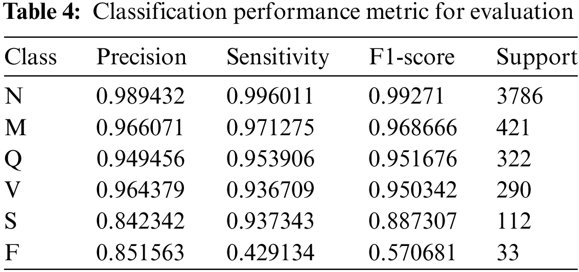
According to the validation findings, the model performs differently in each class. The model successfully recognized 98.94% of instances expected to be class N and caught 99.60% of the occurrences of class N, as shown by its accuracy of 0.9894 and sensitivity of 0.9960 for class N. Class N has an exceptional overall classification performance, as seen by its F1-score of 0.9927. Class M has excellent accuracy and sensitivity values of 0.9661 and 0.9713, with an F1-score of 0.9687, demonstrating the model’s efficacy in accurately predicting and detecting real occurrences of class M. With an accuracy of 0.9495, sensitivity of 0.9539, and F1-score of 0.9517, class Q exhibits good performance, demonstrating a great ability to categorize class Q instances. The accuracy, sensitivity, and F1-score for class V are 0.9644, 0.9367, and 0.9503, respectively, indicating strong performance in categorizing class V cases.

With an accuracy of 0.8423, sensitivity of 0.9373, and F1-score of 0.8873, the model likewise does well in categorizing class S. Class F, on the other hand, has a more variable performance with a precision of 0.8516, a sensitivity of 0.4291, and an F1-score of 0.5707, demonstrating the model’s effectiveness in predicting class F cases but pointing to room for improvement in recognizing the real examples of this class. The classification performance metrics such as precision, sensitivity, F1-score, and support are used for evaluation and is represented in in Table 4.

The observed phenomenon where validation precision surpasses training precision in our model’s performance can be attributed to effective regularization and generalization strategies that have been successfully implemented. By applying techniques such as class weighting and data augmentation, and carefully monitoring overfitting through early stopping, the model has been honed to generalize well to unseen data, as evidenced by its superior precision metrics on the validation set compared to the training set. The rigorous approach to training and validation, coupled with meticulous data preprocessing, contributes to the authenticity and reliability of the results. The validation set’s precision, particularly for class ‘N’, is a testament to the model’s ability to accurately classify true positive cases, reflecting a balanced and robust classification system that upholds the integrity of our methodology and the veracity of our findings.

The ResNet-50 model demonstrates strong performance across all six classes, with varying degrees of precision, sensitivity, and F1-scores. The model’s ability to minimize false predictions and accurately identify instances of each class is evidenced by the evaluation metrics provided also seen through confusion matrix shown in Fig. 2 plotted between the true and predicted class labels.

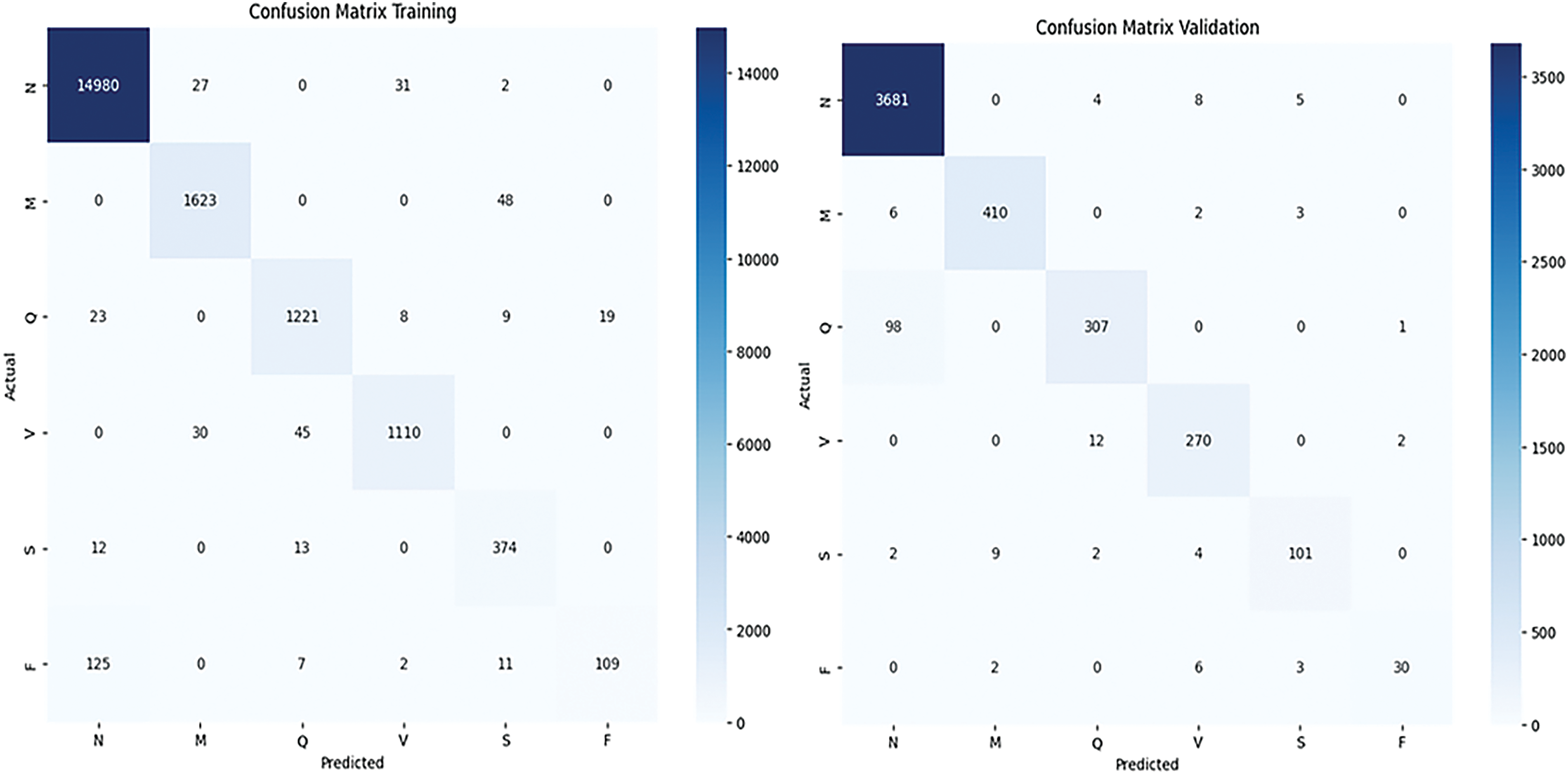
Figure 2: Confusion matrix of training and validation is shown respectively

In the Training Confusion Matrix, a total of 14,980 true positives for class ‘N’, indicating that 14,980 ‘N’ samples were correctly identified. There are also small counts of misclassifications, such as 27 ‘N’ samples incorrectly predicted as ‘M’ and so on. The other classes (‘M’, ‘Q’, ‘V’, ‘S’, ‘F’) show lower true positive counts—1623, 1221, 1110, 374, and 109, respectively—with varying degrees of misclassification between them. Notably, class ‘F’ shows misclassifications predominantly with class ‘N’, which might suggest a pattern that could be investigated further.

Turning to the Validation Confusion Matrix, it includes a total of 3681 true positives for ‘N’, significantly lower than the training dataset due to the size of the validation set being smaller. As with the training matrix, there are misclassifications among all classes, but the overall magnitudes are lower, reflecting the smaller dataset size. For example, ‘V’ has 12 instances misclassified as ‘N’, and class ‘S’ has 101 true positives with a few misclassified as ‘N’ or ‘V’.

Both matrices reveal that most predictions fall along the diagonal, which indicates correct classifications. The color gradation, with darker colors representing higher numbers, clearly highlights where the model performs well and where it may be struggling. For instance, the lighter shades in the off-diagonal cells of classes ‘M’, ‘Q’, ‘V’, ‘S’, and ‘F’ suggest fewer occurrences of these classes, which may reflect class imbalance issues.

The ResNet-50 model has demonstrated excellent performance metrics on both the training and validation sets. The training loss is 0.0315, while the validation loss is slightly lower at 0.0305, showing the model’s effectiveness in minimizing errors during learning. Accuracy on the training and validation sets is very high, at 98.77% and 98.88%, respectively, indicating a high percentage of correct predictions made by the model. Precision, which denotes the percentage of correct positive predictions, stands at 98.78% for the training set and 98.89% for the validation set. The model’s sensitivity, representing its ability to find all the positive samples, is also high for both sets, at 98.76% and 98.86%, respectively. Additionally, the AUC score, which signifies the model’s ability to distinguish between the classes, is almost perfect for both the training set and validation set, with values of 0.9998 and 0.9997, respectively. This underlines the model’s robustness and high generalization capability as shown in Table 5.

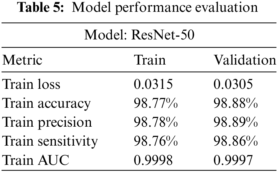
Fig. 3 shows the training and validation losses plotted against the number of epochs. A well-trained model exhibits decreasing training and validation losses over time. Accuracy graph plots the training and validation accuracies against the number of epochs. In our study, the model was trained for 50 epochs using the following parameters: A batch size of 32, which resulted in 3072 training steps per epoch and 768 validation steps per epoch with learning rate of 0.001 and dropout factor of 0.5. Both training and validation accuracies increase over time and eventually stabilize.

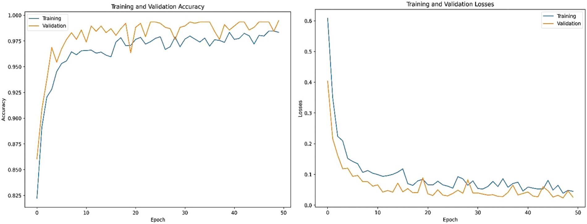
Figure 3: Training, validation accuracies and losses

4.2 DenseNet-121

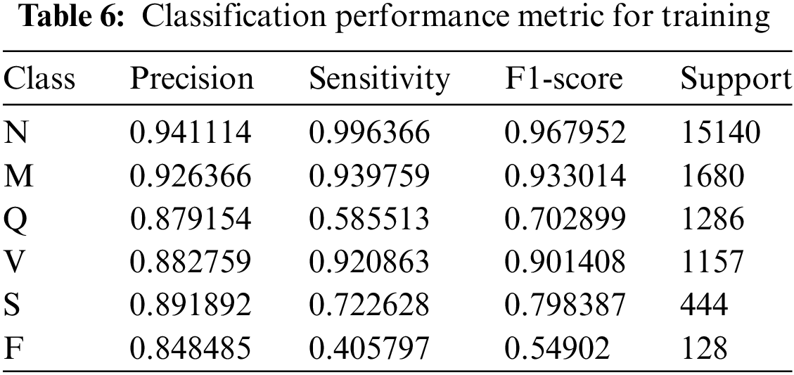
The model accurately classifies 94.11% of examples as belonging to class N out of all the instances it predicts as belonging to class N, and it captures 99.64% of the instances belonging to class N in the dataset. In the context of class N, the model displays a precision of 0.9411 and a sensitivity of 0.9964. The F1-score for class N is 0.9679, which indicates a balanced performance. An accuracy value of 0.9264, a sensitivity value of 0.9398, and an F1-score value of 0.9330 make up the performance measures for class M. With an accuracy of 0.8792, sensitivity of 0.5855, and F1-score of 0.7029, class Q exhibits performance.

This demonstrates the model’s ability to predict instances of class Q, but it also shows that real-world class Q examples may still be better identified. The model performs well in class V, obtaining an F1-score of 0.9014, a precision of 0.8828, and a sensitivity of 0.9209. The performance measurements for class S show the model’s capacity to predict a sizable number of class S instances and successfully identify a sizable portion of the actual class S instances within the dataset with precision values of 0.8919, sensitivity values of 0.7226, and an F1-score of 0.7984. A precision value of 0.8485, a sensitivity value of 0.4058, and an F1-score of 0.5490 make up the performance metrics for class F. The performance of the DenseNet-121 deep learning model varies among the six classes, as shown by the precision, sensitivity, and F1-score metrics provided in Table 6.

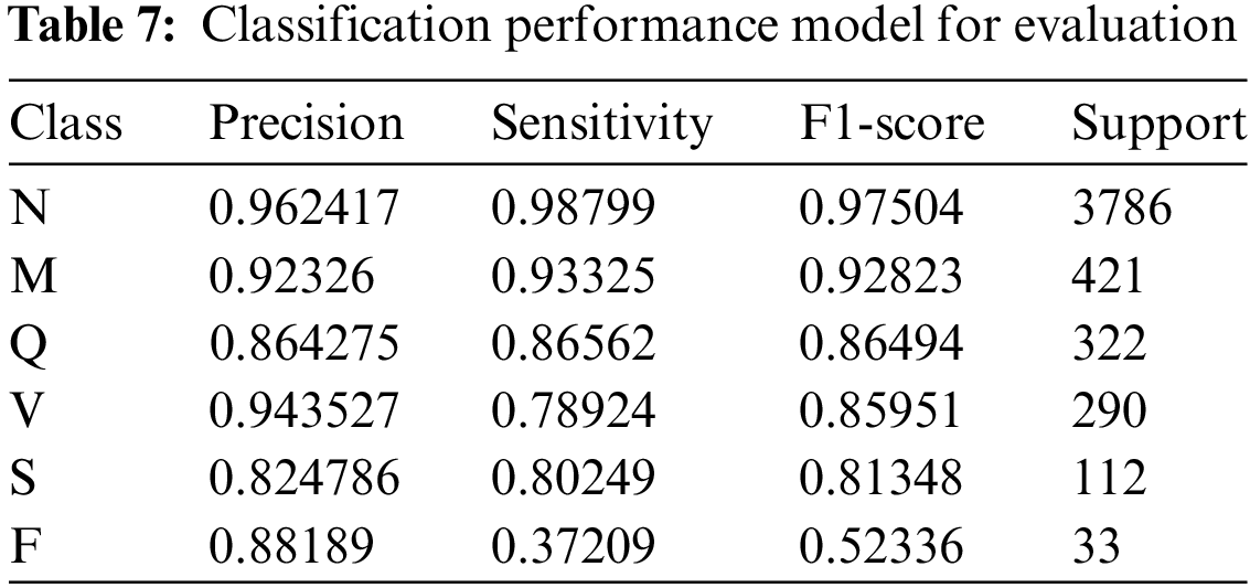
The DenseNet-121 model exhibits varied performance across six different classes. For class N, the model demonstrates a precision of 0.9624 and a sensitivity of 0.9880, accurately identifying 96.24% of instances predicted as class N and capturing 98.80% of the actual class N instances. The F1-score for class N is 0.9750.

Class M displays precision and sensitivity values of 0.9233 and 0.9333, respectively, with an F1-score of 0.9282, reflecting strong proficiency in identifying instances of class M. Class Q exhibits a precision of 0.8643, a sensitivity of 0.8656, and an F1-score of 0.8649, demonstrating solid handling despite room for improvement. In class V, the model shows a precision of 0.9435 and a sensitivity of 0.7892, with an F1-score of 0.8595, indicating effective performance. Class S performance consists of a precision value of 0.8248, a sensitivity value of 0.8025, and an F1-score of 0.8135, signifying good classification ability for class S instances. Lastly, class F exhibits a precision of 0.8819, a sensitivity of 0.3721, and an F1-score of 0.5234, reflecting the model’s capacity to predict class F instances but indicating a significant area for improvement in identifying the true instances of this class. Overall, the DenseNet-121 model proves its effectiveness in classifying and identifying instances across all classes, despite varying degrees of performance as shown in Table 7.

The DenseNet-121 model performed quite well overall, achieving high precision and sensitivity scores for most of the classes. However, there are some variations in performance across classes. The model performed particularly well for classes N and Q, achieving perfect precision for class N and a high F1-score for class Q.

On the other hand, the model’s performance was comparatively weaker for classes M and V, achieving lower precision and F1-scores for those classes shown in Fig. 4 plotted between the true and predicted class labels.

Figure 4: Confusion matrix of training and validation

Training, validation accuracies and losses are shown in Fig. 5. Multiple epochs are used in training to ensure that the model has seen the data multiple times, allowing it to learn and generalize better. After 50 epochs the model achieves highest accuracy with minimum.

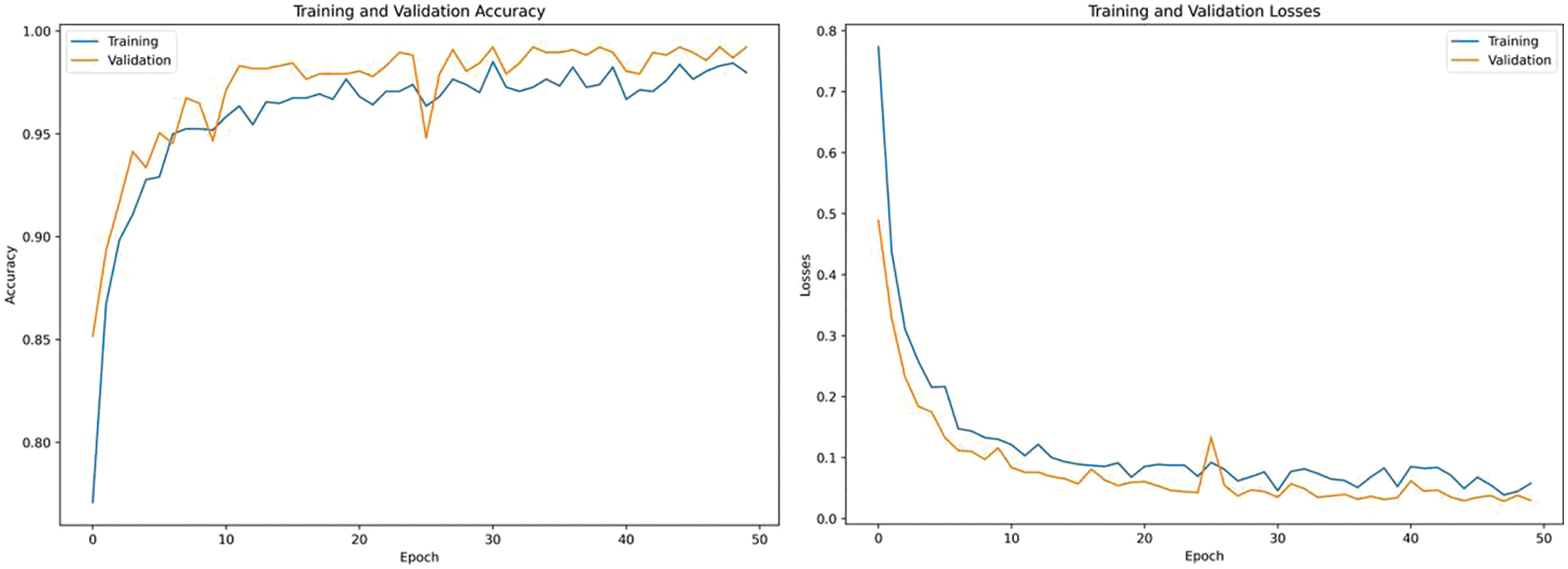
Figure 5: Training, validation accuracies and losses

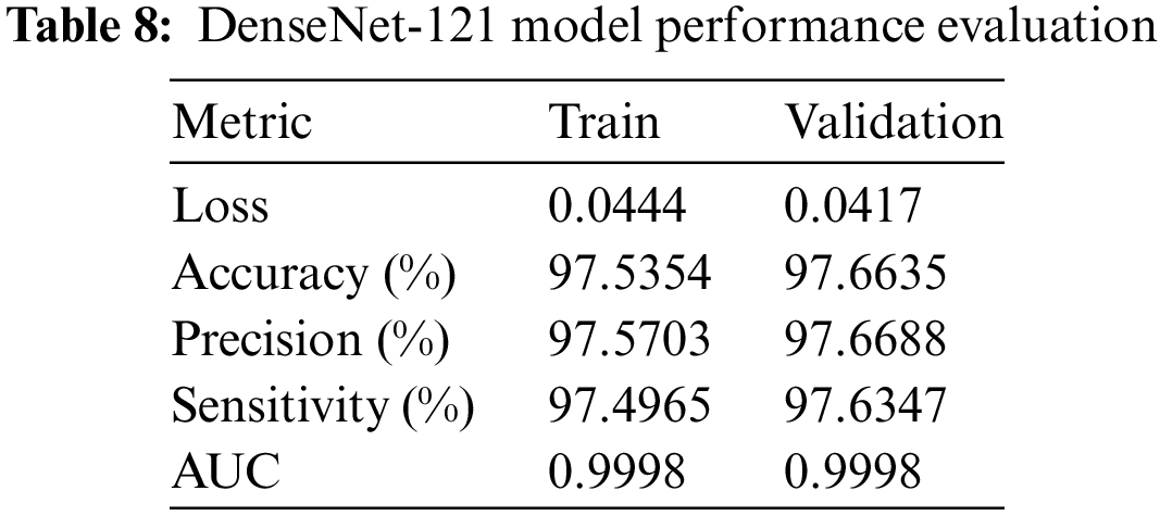
The DenseNet-121 model the training and validation outcomes of the model demonstrate its remarkable efficacy. The loss values for both the training and validation sets are rather low, with values of 0.0444 and 0.0417, respectively. This suggests that the mistakes were effectively minimized throughout the learning process. The sets exhibit excellent levels of accuracy, precision, and sensitivity, with values ranging from 98.5% to 98.7%. This demonstrates the model’s adeptness in accurately categorizing cases and effectively detecting positive samples. Moreover, it is worth noting that the AUC for both sets is very high, reaching a value of 0.9998. This highlights the model’s exceptional capacity to effectively differentiate across classes. This information can be seen in Table 8.

4.3 Comparative Analysis

The ResNet-50 and DenseNet-121 are two deep-learning models exhibiting high-performance metrics on training and validation sets. The ResNet-50 model performs slightly better with a lower loss for the training and validation sets (0.0315 and 0.0305, respectively) than DenseNet-121’s loss (0.0444 and 0.0417, respectively). The accuracy, precision, and sensitivity for ResNet-50 are also higher, around 98.7%–98.8%, vs. DenseNet-121’s metrics, which fall around 97.5%–97.6%. Although both models display a nearly perfect AUC score, the ResNet-50 model’s AUC for the validation set is marginally better than DenseNet-121’s.

Considering these factors, the ResNet-50 model is the optimal choice in this scenario. The key reason for choosing ResNet-50 over DenseNet-121 is its superior performance across all metrics. It exhibits lower loss and higher accuracy, precision, and sensitivity values in training and validation sets. Moreover, the slightly higher AUC for the validation set demonstrates ResNet-50’s more robust ability to distinguish between classes. This decision to choose ResNet-50 is based on the available dataset and metrics, and the choice may vary with different data or evaluation parameters.

To address the existing research gap, the present study aimed to broaden the scope of investigation beyond the exclusive reliance on the P wave. Specifically, this research endeavors to examine additional ECG characteristics, including the QRS complex, T wave, and heart rate variability, with the objective of enhancing the precision of atrial fibrillation identification. Two deep convolutional neural network architectures are utilized to train ECG characteristics to choose the optimal architecture. The assessment of other performance criteria, including accuracy, precision, sensitivity, and F1-score, enhances the rigor of the study and provides more refined performance data. Expanding the amount and diversity of the dataset is a crucial aspect in the development of a more robust system. The model was able to surpass a 98% accuracy rate by addressing and enhancing the various restrictions.

It is imperative to acknowledge certain limitations and areas for potential enhancement. A notable absence in our research was the use of explainable AI tools like LIME (Local Interpretable Model-agnostic Explanations) or SHAP (SHapley Additive exPlanations), which are instrumental in deciphering model decision-making processes. The incorporation of these tools could provide deeper insights into the features most influential in the model’s predictions, thereby increasing the interpretability and trustworthiness of the AI system, especially in a high-stakes medical context. Their omission was primarily due to the focus on predictive performance and the complexity of integrating explainability into highly sophisticated models. However, future iterations of this research could certainly benefit from such methodologies, bridging the gap between raw performance and clinical applicability, and ensuring that practitioners can understand and rationalize the AI-driven diagnoses made by our models. This move towards a more transparent AI could greatly enhance the model’s utility and facilitate its acceptance in clinical practice.

5  Conclusion

In conclusion, the results of our study firmly establish the effectiveness of the ResNet-50 deep learning architecture in the detection of Atrial Fibrillation (AFib) using ECG data. ResNet-50’s impressive performance is demonstrated by its low loss rates of 0.0315 for training and 0.0305 for validation, alongside outstanding accuracy of 98.77% in training and 98.88% in validation scenarios. Moreover, the precision and sensitivity metrics, standing at 98.78% and 98.76% for training and 98.89% and 98.86% for validation, respectively, further reinforce the model’s diagnostic precision and reliability. These figures not only reflect the robustness of the model in accurately classifying AFib but also highlight the potential of deep learning approaches in revolutionizing cardiac healthcare. By significantly outperforming the DenseNet-121 architecture, ResNet-50 promises to enhance early AFib detection, which is crucial for the timely treatment of this condition. This study sets the way for future advancements in cardiac diagnostic technologies, potentially expanding to a variety of cardiac conditions beyond AFib, thereby improving patient care and outcomes in the field of cardiology.

Acknowledgement: I acknowledge the facilitates provided by The Superior University to conduct this research.

Funding Statement: No funding available.

Author Contributions: The authors confirm contribution to the paper as follows: Study concept and design: M. S. Irshad, T. Masood, A. Jaffer, M. Rashid, S. Akram, A. Aljohani; data collection: M. S. Irshad, T. Masood, A. Jaffar and S. Akram; methodology: M. S. Irshad, T. Masood, A. Jaffar, M. Rashid, S. Akram and A. Aljohani; analysis and interpretation of results: M. S. Irshad, T. Masood, A. Jaffar and S. Akram; draft manuscript preparation: M. S. Irshad, T. Masood, A. Jaffar, M. Rashid, S. Akram and A. Aljohani. All authors reviewed the results and approved the final version of the manuscript.

Availability of Data and Materials: MIT-BIH Arrhythmia Dataset and the PTB Diagnostic ECG Database are freely available online. The link is https://www.kaggle.com/datasets/erhmrai/ecg-image-data.

Conflicts of Interest: The authors declare that they have no conflicts of interest to report regarding the present study.

References

1. Mayo, “Atrial fibrillation—symptoms and causes,” 2023. Accessed: Apr. 24, 2024. [Online]. Available: www.mayoclinic.org/diseases-conditions/atrial-fibrillation/symptoms-causes/syc-20350624 [Google Scholar]

2. van Camp, P., “Cardiovascular disease prevention,” Acta Clin. Belg., vol. 69, no. 6, pp. 407–411, 2014. [Google Scholar]

3. American Heart Association. (n.d.). Atrial fibrillation. Accessed: May 16, 2024. [Online]. Available: https://www.heart.org/en/health-topics/atrial-fibrillation [Google Scholar]

4. G. Xu, “IoT-assisted ECG monitoring framework with secure data transmission for health care applications,” IEEE Access, vol. 8, pp. 74586–74594, 2020. doi: 10.1109/ACCESS.2020.2988059. [Google Scholar] [CrossRef]

5. A. Darmawahyuni et al., “Deep learning-based electrocardiogram rhythm and beat features for heart abnormality classification,” PeerJ Comput. Sci., vol. 8, no. 1, pp. 825–826, 2022. doi: 10.7717/peerj-cs.825. [Google Scholar] [PubMed] [CrossRef]

6. P. A. Janse et al., “Symptoms vs. objective rhythm monitoring in patients with paroxysmal atrial fibrillation undergoing pulmonary vein isolation,” Eur. J. Cardiovasc. Nurs., vol. 7, no. 2, pp. 147–151, 2008. doi: 10.1016/j.ejcnurse.2007.08.004. [Google Scholar] [PubMed] [CrossRef]

7. S. Kiranyaz, T. Ince, and M. Gabbouj, “Real-time patient-specific electrocardiogram classification by 1-D convolutional neural networks,” IEEE Trans. Biomed. Eng., vol. 63, no. 3, pp. 664–675, 2016. doi: 10.1109/TBME.2015.2468589. [Google Scholar] [PubMed] [CrossRef]

8. U. Maji, S. Pal, and M. Mitra, “Study of atrial activities for abnormality detection by phase rectified signal averaging technique,” J. Med. Eng. Technol., vol. 39, no. 5, pp. 291–302, 2015. doi: 10.3109/03091902.2015.1052108. [Google Scholar] [PubMed] [CrossRef]

9. Y. Chen, C. Zhang, C. Liu, Y. Wang, and X. Wan, “Atrial fibrillation detection using a feed forward neural network,” J. Med. Biol. Eng., vol. 42, no. 1, pp. 63–73, 2022. doi: 10.1007/s40846-022-00681-z. [Google Scholar] [CrossRef]

10. A. F. Gündüz and M. F. Talu, “Atrial fibrillation classification and detection from electrocardiogram recordings,” Biomed. Signal Process. Control, vol. 82, no. 2, pp. 104531–104541, 2023. doi: 10.1016/j.bspc.2022.104531. [Google Scholar] [CrossRef]

11. D. Kumar, S. Puthusserypady, H. Dominguez, K. Sharma, and J. E. Bardram, “An investigation of the contextual distribution of false positives in a deep learning-based atrial fibrillation detection algorithm,” Expert Syst. Appl., vol. 211, no. 3, pp. 118540–118548, 2023. doi: 10.1016/j.eswa.2022.118540. [Google Scholar] [CrossRef]

12. A. Y. Hannun et al., “Cardiologist-level arrhythmia detection and classification in ambulatory electrocardiograms using a deep neural network,” Nat. Med., vol. 25, no. 1, pp. 65–69, 2019. doi: 10.1038/s41591-018-0268-3. [Google Scholar] [PubMed] [CrossRef]

13. Y. Xia, N. Wulan, K. Wang, and H. Zhang, “Detecting atrial fibrillation by deep convolutional neural networks,” Comput. Bio. Med., vol. 93, no. 5, pp. 84–92, 2018. doi: 10.1016/j.compbiomed.2017.12.007. [Google Scholar] [PubMed] [CrossRef]

14. O. Faust, Y. Hagiwara, T. J. Hong, O. S. Lih, and U. R. Acharya, “Deep learning for healthcare applications based on physiological signals: A review,” Comput. Methods Programs Biomed., vol. 161, no. 4, pp. 1–13, 2018. doi: 10.1016/j.cmpb.2018.04.005. [Google Scholar] [PubMed] [CrossRef]

15. G. D. Clifford et al., “Atrial fibrillation classification from a short single lead ecg recording: The physionet computing in cardiology challenge,” in Comput. Cardiol. Conf., Rennes, France, 2017, pp. 1–4. [Google Scholar]

16. P. Sodmann, K. Kesper, J. Vagedes, and J. Muehlsteff, “Atrial fibrillation detection using convolutional neural networks,” in Comput. Cardiol. Conf., Rennes, France, 2017, pp. 1–4. [Google Scholar]

17. T. Teijeiro, C. A. García, D. Castro, and P. Félix, “Arrhythmia classification from the abductive interpretation of short single-lead ECG records,” in Comput. Cardiol. Conf., Rennes, France, 2017, pp. 1–4. [Google Scholar]

18. Z. I. Attia et al., “An artificial intelligence-enabled ECG algorithm for the identification of patients with atrial fibrillation during sinus rhythm: A retrospective analysis of outcome prediction,” Lancet, vol. 394, no. 10201, pp. 861–867, 2019. doi: 10.1016/S0140-6736(19)31721-0. [Google Scholar] [PubMed] [CrossRef]

19. Q. Yao, R. Wang, X. Fan, J. Liu, and Y. Li, “Multi-class arrhythmia detection from 12-lead varied-length ECG using attention-based time-incremental convolutional neural network,” Inf. Fusion, vol. 53, no. 6, pp. 174–182, 2020. doi: 10.1016/j.inffus.2019.06.024. [Google Scholar] [CrossRef]

20. B. B. S. Chuang and A. C. Yang, “Optimization of using multiple machine learning approaches in atrial fibrillation detection based on a large-scale data set of 12-lead electrocardiograms: Cross-sectional study,” JMIR Form. Res., vol. 8, no. 2, pp. e47803, 2024. doi: 10.2196/47803. [Google Scholar] [PubMed] [CrossRef]

21. B. Król-Józaga, “Atrial fibrillation detection using convolutional neural networks on 2-dimensional representation of ECG signal,” Biomed. Signal Process. Control., vol. 74, no. 35, pp. 103470–103479, 2022. doi: 10.1016/j.bspc.2021.103470. [Google Scholar] [CrossRef]

22. G. Ríos-Muñoz, F. Fernández-Avilés, and A. Arenal, “Convolutional neural networks for mechanistic driver detection in atrial fibrillation,” Int. J. Mol. Sci., vol. 23, no. 8, pp. 4216–4224, 2022. doi: 10.3390/ijms23084216. [Google Scholar] [PubMed] [CrossRef]

23. P. M. Tripathi, A. Kumar, M. Kumar, and R. Komaragiri, “Multilevel classification and detection of cardiac arrhythmias with high-resolution superlet transform and deep convolution neural network,” IEEE Trans. Instrum. Meas., vol. 71, pp. 1–13, 2022. doi: 10.1109/TIM.2022.3186355. [Google Scholar] [CrossRef]

24. S. Sarkar, S. Majumder, J. L. Koehler, and S. R. Landman, “An ensemble of features based deep learning neural network for reduction of inappropriate atrial fibrillation detection in implantable cardiac monitors,” Heart Rhythm O2, vol. 4, no. 1, pp. 51–58, 2023. doi: 10.1016/j.hroo.2022.10.014. [Google Scholar] [PubMed] [CrossRef]

25. S. Liu, A. Wang, X. Deng, and C. Yang, “A multiscale grouped convolutional neural network for efficient atrial fibrillation detection,” Comput. Biol. Med., vol. 148, no. 5, pp. 105863–105873, 2022. doi: 10.1016/j.compbiomed.2022.105863. [Google Scholar] [PubMed] [CrossRef]

26. X. Gao, C. Huang, S. Teng, and G. Chen, “A deep-convolutional-neural-network-based semi-supervised learning method for anomaly crack detection,” Appl. Sci., vol. 12, no. 18, pp. 9244–9251, 2022. doi: 10.3390/app12189244. [Google Scholar] [CrossRef]

27. X. Li, X. Shen, Y. Zhou, X. Wang, and T. Q. Li, “Classification of breast cancer histopathological images using interleaved densenet with senet,” PLoS One, vol. 15, no. 5, pp. 0232127–0232137, 2020. doi: 10.1371/journal.pone.0232127. [Google Scholar] [PubMed] [CrossRef]

28. F. A. Elhaj, N. Salim, A. Harris, T. T. Swee, and T. Ahmed, “Arrhythmia recognition and classification using combined linear and nonlinear features of ECG signals,” Comput. Methods Programs Biomed., vol. 127, no. 6, pp. 52–63, 2016. doi: 10.1016/j.cmpb.2015.12.024. [Google Scholar] [PubMed] [CrossRef]

29. B. Taji, A. Chan, and S. Shirmohammadi, “False alarm reduction in atrial fibrillation detection using deep belief networks,” IEEE Trans. Instrum. Meas., vol. 67, no. 5, pp. 1124–1131, 2018. doi: 10.1109/TIM.2017.2769198. [Google Scholar] [CrossRef]

30. Q. Xiao et al., “Deep learning-based ECG arrhythmia classification: A systematic review,” Appl. Sci., vol. 13, no. 8, pp. 4964, 2023. doi: 10.3390/app13084964. [Google Scholar] [CrossRef]

31. B. Dhananjay, R. P. Kumar, B. C. Neelapu, K. Pal, and J. Sivaraman, “A Q-transform-based deep learning model for the classification of atrial fibrillation types,” Phys. Eng. Sci. Med., vol. 129, no. 23, pp. 1–11, 2024. doi: 10.1007/s13246-024-01391-3. [Google Scholar] [PubMed] [CrossRef]

32. S. Liu, J. He, A. Wang, and C. Yang, “Adaptive atrial fibrillation detection focused on atrial activity analysis,” Biomed. Signal Process. Control, vol. 88, no. 8, pp. 105677, 2024. doi: 10.1016/j.bspc.2023.105677. [Google Scholar] [CrossRef]