Vehicle Abnormal Behavior Detection Based on Dense Block and Soft Thresholding

1  Introduction

With the rapid development of the national economy and the rapid growth of domestic car ownership, cars not only bring convenience to people’s travel but also bring many security risks. Effective traffic system management is crucial for ensuring both the safety and efficiency of transportation. In recent years, the rapid advancement of artificial intelligence across various sectors has prompted researchers to explore AI-based methods for traffic system management. Intelligent Transportation System (ITS) [1–3] is an important measure of traffic management, which can effectively integrate advanced computer vision processing and communication technology into the entire traffic management system. This integrated management system allows for the comprehensive, real-time, accurate, and efficient monitoring and management of various types of vehicles, and it can also predict the future trajectories of traffic participants based on actual data [4]. As an important traffic management technology, vehicle abnormal behavior detection is an indispensable part of intelligent transportation system. On the one hand, vehicle abnormal behavior recognition technology can reduce the pressure on traffic management personnel and reduce the waste of human resources. On the other hand, it can enhance the efficiency, accuracy, and timeliness of traffic monitoring.

Vehicle abnormal behavior detection [5,6], a subset of traffic incident detection, identifies incidents such as traffic violations and accidents. At present, the detection methods of vehicle abnormal behavior are mainly based on video recognition. These methods [7,8] use cameras to capture real-time video data of traffic, which is then analyzed through video and image processing to detect traffic flow or to track and identify targets. The vehicle detection method based on video image processing offers a large detection range and rich information. The detection system itself only needs to have a camera, processor, and other basic units, the hardware equipment is simple, easy to install and maintain, cost-effective, durable, and easy to upgrade. Therefore, traffic flow detection based on video images has become a research focus worldwide.

Due to the complexity of urban road traffic conditions, mature vehicle behavior detection algorithms are mainly applied to highways and expressways. However, most traffic accidents occur on urban roads, where the environment is more prone to abnormal events, leading to severe consequences. Therefore, the rapid and accurate detection of abnormal vehicle behaviors on urban roads is critical for saving lives, reducing property losses, alleviating congestion, and providing timely warnings. To address these challenges, we designed a new abnormal traffic behavior recognition model. The main contributions of this paper are summarized as follows:

1.   We use R3D as the backbone network for spatial feature extraction, and improve model accuracy by fully learning 3D spatio-temporal features within input video frames.

2.   Through experiments, we find a spatial feature extraction method that is more suitable for abnormal behavior detection of surveillance video. We employ dense blocks to extract spatial features from surveillance video. This allows the network to make the most of existing features and learn new ones without adding additional computations. We then filter the noise using soft thresholds and pass the extracted features to the next part of the network. The soft thresholds are adaptable based on current traffic conditions, thus enhancing the network’s flexibility.

3.   We use Bi-LSTM to receive spatial features extracted from the upper layer and further extract temporal information from it. The training of Bi-LSTM further improves the recognition ability of the network, and the recognition accuracy rate, and finally outputs the recognition result.

4.   The rest of this article is described below. Chapter 2 introduces the existing research methods based on traditional methods and deep learning. The shortcomings and improvement directions of these methods are also pointed out. Chapter 3 describes the principles of the networks, algorithms, and techniques used in this article. In Chapter 4, the data set used in this paper is presented, and all the experiments are compared and analyzed.

2  Related Work

Vehicle abnormal behavior detection can be broadly classified into indirect and direct methods. Among them, the indirect method is to use the ground sensor [9,10] to obtain changes in traffic parameters and indirectly identify traffic events by using methods such as pattern recognition or statistical analysis. This type of method is more suitable for traffic congestion events under high traffic flow. However, due to the influence of the detector installation location, it is powerless in the recognition of vehicle abnormal behavior in other locations, such as illegal parking, speeding, vehicle reversing, and other specific vehicle behavior. Thus, the indirect method cannot meet the diverse traffic event recognition applications that occur on urban roads.

The method of directly identifying vehicle abnormal behavior events using video image processing technology is called the direct method. With the development of image processing, pattern recognition, and artificial intelligence technology, vehicle abnormal behavior recognition methods based on image processing [11–13] can acquire road scene image information through visual sensors. Computer image processing technology and pattern recognition technology are used to analyze the collected images for real-time processing and extract traffic information. And the collected information is transmitted to the clients such as the traffic control center through the network transmission system via signal machines. It provides comprehensive and real-time traffic status information for urban traffic management and control.

The direct method based on image processing has the advantages of high intuitiveness, good real-time performance, and high reliability compared with the indirect method. Moreover, it can detect a wide range of events, the variety of recognizable events is rich, and the events have repeatability and reproducibility. Therefore, it has received wide attention from domestic and foreign research scholars.

Wang et al. combined time series analysis (TSA) with a Support Vector Machine (SVM) [14–16] in 2013. The time series component predicts traffic volumes, and the SVM component detects events based on real-time traffic volumes, predicted normal traffic volumes, and the difference between the two. The results show that this algorithm has a high detection rate, but also a high false alarm rate, and the neural network structure is too large, requiring large storage space and long computation time. In 2019, Li et al. proposed a GAN-RF-SVM-based event detection model [17] under small sample conditions. New event samples are generated using a generative adversarial network (GAN) and variables are selected using a random forest (RF) algorithm. Finally, SVM is used as the event detection model. This solves the problems of small sample size, unbalanced sample size, and poor real-time performance in accident detection systems, and reduces the false alarm rate of traffic accident detection. The main drawback of this algorithm is that the portability is poor and the performance of testing detection on different road sections is significantly reduced. In the detection of traffic videos, detecting small objects has always been one of the key challenges in vehicle detection. Li et al. [18] proposed a novel multi-scale detection network based on a differential segmentation criterion, which significantly improves the detection rate of small objects compared to traditional methods. The implementation of indirect and direct methods requires data collection by detectors. To address the issue of modern detectors’ poor adaptability to actual complex traffic environments, Zhang et al. [19] introduced a Category-Induced Coarse-to-Fine Domain Adaptation Approach (C2FDA) method that significantly enhances the adaptability of detectors in new, unseen domains.

Research-based on high-dimensional time series analysis and anomaly detection [20] is a new development in recent years regarding the identification of anomalous traffic behaviors. The study proposes a method to address the challenge of ensuring the reliability of vehicle systems in the face of the growing complexity of modern vehicles. By combining a Multi-Layer Long Short Term Memory (LSTM) network with an Autoencoder architecture (ML-LSTMAE), the approach accurately analyzes the operation of various vehicle subsystems through training an encoding-decoding scheme using multivariate time series data. Additionally, the method utilizes a One-Class Support Vector Machine (OCSVM) to analyze reconstruction errors and establish a support boundary to differentiate between healthy and unhealthy states. Validation with real-world vehicle data and NASA bearing data confirms the high accuracy and effectiveness of the proposed approach.

3  Proposed Method

3.1 DRN Block

Based on previous experiments on deep learning, we can conclude that the recognition accuracy of the network is related to the number of layers of the network. Generally, deeper networks tend to perform better due to their increased learning capabilities. However, excessively deep networks are prone to the vanishing gradient problem, where gradients diminish as they propagate back through the layers during training. This issue can halt the updating of network parameters, leading to a decline in recognition accuracy. To solve this problem, we introduced the residual block [21,22], as shown in Fig. 1.

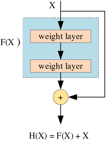
Figure 1: Residual block

H(X) = F(X) + X is the objective function of the residual block. When the network has a vanishing gradient, F(X) approaches 0 and the objective function can be approximated as H(X) = X. This achieves a constant mapping of the output of the network to X, keeping the network as it is and avoiding network degradation. Since the derivative of X has a value of 1, the derivative of H(X) is always greater than or equal to 1 during the back-propagation of the network parameters. This avoids the appearance of a vanishing gradient and allows the network parameters to be updated.

Traditional deep residual networks require a large number of convolutional layers to produce good recognition results. However, as the number of convolutional layers increases, the network suffers from an excessive number of parameters and high computational costs, which greatly increases the training time of the network. In addition, traditional residual networks use a 2D convolution. This can only extract spatial features in the image, and not extract temporal features in the video. For the network to better understand the information in the video, we also need the network to extract the temporal features. To solve the above problem, this paper uses a R3D network instead of 2D convolution and incorporates dense block [23,24]. The Dense-R3D Network (DRN) is shown in Fig. 2.

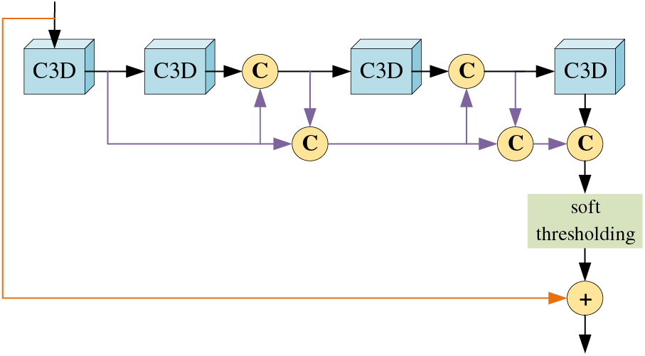
Figure 2: DRN block

As shown in the figure, we have added a dense block to the residual block. We let each group of feature maps converge in the channel dimension before they enter the convolution layer. This achieves feature reuse and allows the network to use a smaller number of features to achieve better recognition results. In feature map convergence, we use concatenation in the channel dimension instead of summation. And these new feature maps are necessary for the model to learn new features, we cannot discard them. So even though each convolutional layer only outputs a very small number of new feature maps, the model still produces a large number of parameters as the number of layers in the network increases. And because for the feature maps to be connected in the channel dimension, we need to ensure that the feature maps are of the same size. We cannot arbitrarily use convolution and pooling to change the size of the feature maps, so we use bottleneck layers at the end of the model to uniformly change the size of the feature maps. As the network reuses the same feature map several times, this makes the network prone to overfitting during training. Therefore, we use the Dropout to make some parameters deactivate randomly during the training process. During the training phase, certain parameters are made to stop working with a certain probability during the forward propagation of the model, which can effectively avoid overfitting the model.

When classifying samples, there will inevitably be some noise in the samples, and the noise tends to be different across samples even for the same dataset. Therefore, at the end of the block, we also used the soft thresholding method [25]. By removing features with absolute values less than a certain threshold and compressing features with absolute values greater than that threshold in the direction of zero, as shown by Eq. (1).

y={x−τx>τ0−τ≤x≤τx+τx<−τ(1)

As can be seen from the equation, the derivatives of soft thresholds are 0 and 1. So using this method avoids the vanishing gradient and exploding gradient that occurs in deep learning algorithms.

To prevent the output of the soft threshold function from being all 0 or all not 0. we need to set the thresholds all to positive values, and the values cannot be too large. At the same time, to have good portability of the model, the thresholds should be adaptive. Each sample should have its independent threshold value depending on its noise content, and the threshold value is different for each sample. For example, sample A contains less noise, while sample B contains more noise in the same dataset. Therefore, when performing soft thresholding, a larger threshold should be used for sample A and a smaller one for sample B. The specific implementation process is shown in Fig. 3.

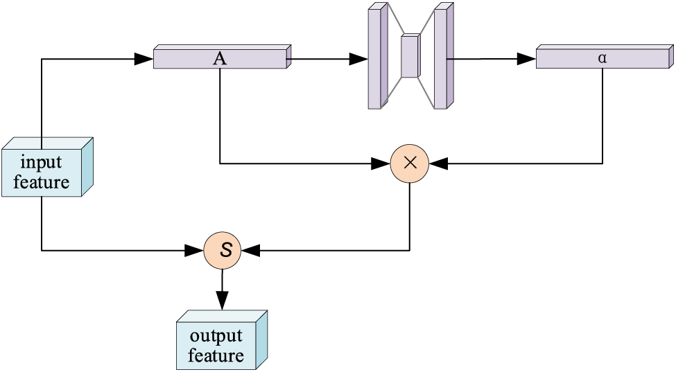
Figure 3: Soft thresholding method

First, we take the absolute value of the input feature map, so that the feature map is guaranteed to have all positive values. We record the resulting new feature map as A. Next, we sent A into a small fully-connected network whose output layer is a Sigmoid function. Using a small number of calculations, the output is normalized to a number between 0 and 1. We record this coefficient as α. α × A is the final threshold. Using this method, the threshold is guaranteed to be positive and not too large in value. Since the threshold for each sample is calculated from its feature map, different samples have different thresholds. This gives the model a high degree of self-adaptability. This algorithm can be understood as a special kind of attention mechanism. It notices features that are not relevant to the current task and removes them by soft thresholding. At the same time features that are relevant to the current task are noticed and they have adapted appropriately.

3.2 LSTM

Long short-term memory (LSTM) [26–28] network is an efficient recurrent neural network, which can better extract temporal feature information. To better extract the temporal features over long distances, we aggregate the output of the DRN block into the LSTM. One of the LSTM units is shown in Fig. 4. The input feature map is rewritten in dimensionality to one dimension. To retain the important features, we input all the features directly into the LSTM for feature extraction.

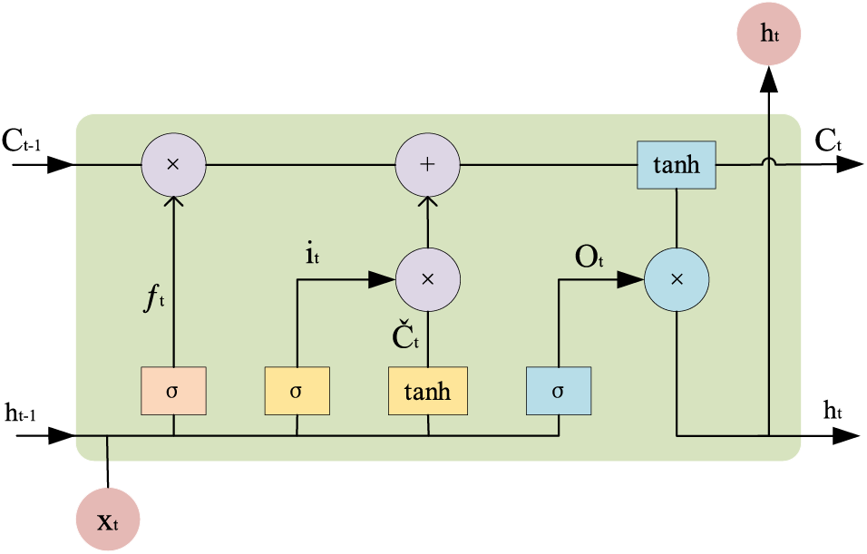
Figure 4: One unit of LSTM

The LSTM consists of three steps, forgetting part of the previous state, updating the memory cell, and outputting the current state. The first step in LSTM is to decide what information we need to forget. This process is done using a forgetting gate. This gate reads the information from ht−1 and xt and outputs a value between 0 and 1 to each data in the cell state Ct−1. 1 means complete retention and 0 means complete discard, as shown in Eq. (2).

ft=σ(Wf×[ht−1,xt]+bf)(2)

The next step is to determine the information we need to update. σ determines the state we want to update, and then tanh creates a new vector of candidate values. C^t will be added to the state and we use these two pieces of information to implement the state update as shown in Eqs. (3) and (4).

it=σ(Wi⋅[ht−1,xt]+bi)(3)

C^t=tanh⁡(WC⋅[ht−1,xt]+bC)(4)

Then, Ct−1 is updated to Ct. We multiply the old state with ft and discard the information we have previously identified as needing to be discarded. Then add it × C^t to form a new candidate value. And updated according to the calculated candidate value, as shown in Eq. (5).

Ct=ft×Ct−1+it×C^t(5)

Finally, the output of the cell state is determined by σ. We process the cell states with tanh and multiply them with the output of σ. The output obtained is shown in Eqs. (6) and (7).

Ot=σ(WO[ht−1]+bO)(6)

ht=Ot×tanh⁡(Ct)(7)

3.3 DRN + Bi-LSTM

The traditional LSTM can only predict the output of the next moment based on the previous feature information. However, in some practical problems, the state at the current moment is not only related to the previous state but may also be related to the future state. We also need to focus on information after the current situation has occurred. Therefore, we build a Bi-LSTM [29,30] network, as shown in Fig. 5, where both A and A’ denote an LSTM cell.

Figure 5: Bi-LSTM network

The image information input undergoes multiple layers of convolution to yield a one-dimensional feature vector, which is then used as the input for the Bi-LSTM. The first layer of the Bi-LSTM receives the extracted features from the left side, allowing the model to understand the current situation by learning the previous spatiotemporal features. The second layer receives the extracted features from the right side, allowing the model to determine current events by future conditions. The second layer is processed in the same way as the first layer but in the opposite direction. Finally, the results obtained from the two layers are judged and analyzed.

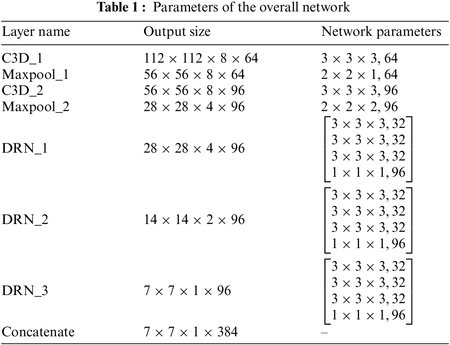
The overall network model structure is shown in Fig. 6. We first use 3D convolution and max pooling operations to transform the input video sequence images into feature maps containing spatiotemporal information and to change the size of the sequence feature maps. Then, we process the input feature maps using multiple DRN modules, dealing with the spatiotemporal information contained in the input feature maps. Since the 3D convolution used by DRN mainly processes short-term temporal information, in order to further enhance the processing of temporal information of the input and improve the model’s ability to handle long-term temporal information, Bi-LSTM is used in the model to extract the temporal information from the sequence of input feature maps. By utilizing the dual-layer structure of Bi-LSTM, bidirectional temporal information in the input feature maps is extracted, and a comprehensive analysis is conducted on the two obtained results. Finally, recognition and classification are carried out based on the processed spatiotemporal feature weight information, and the recognition results are outputted. The specific structure of the network is shown in Table 1.

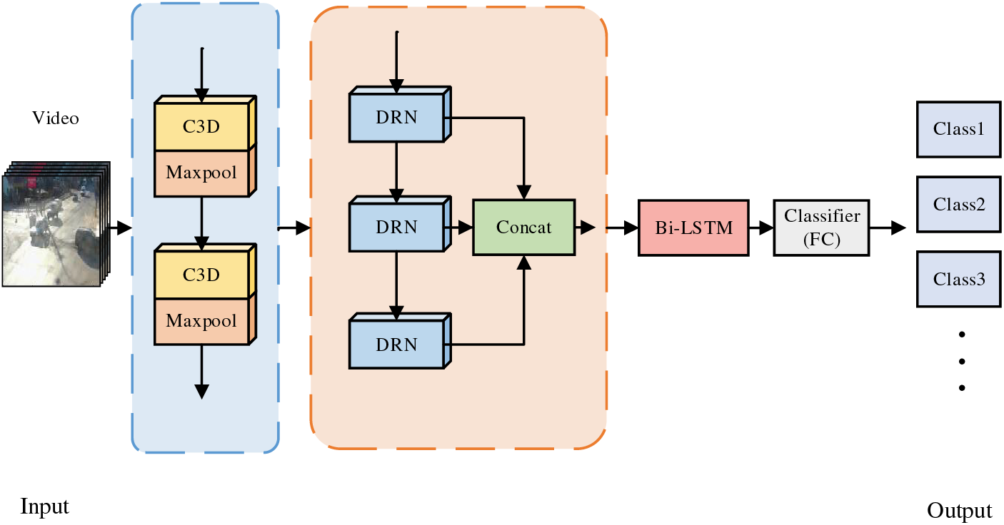
Figure 6: Overall network model

4  Experimental Results

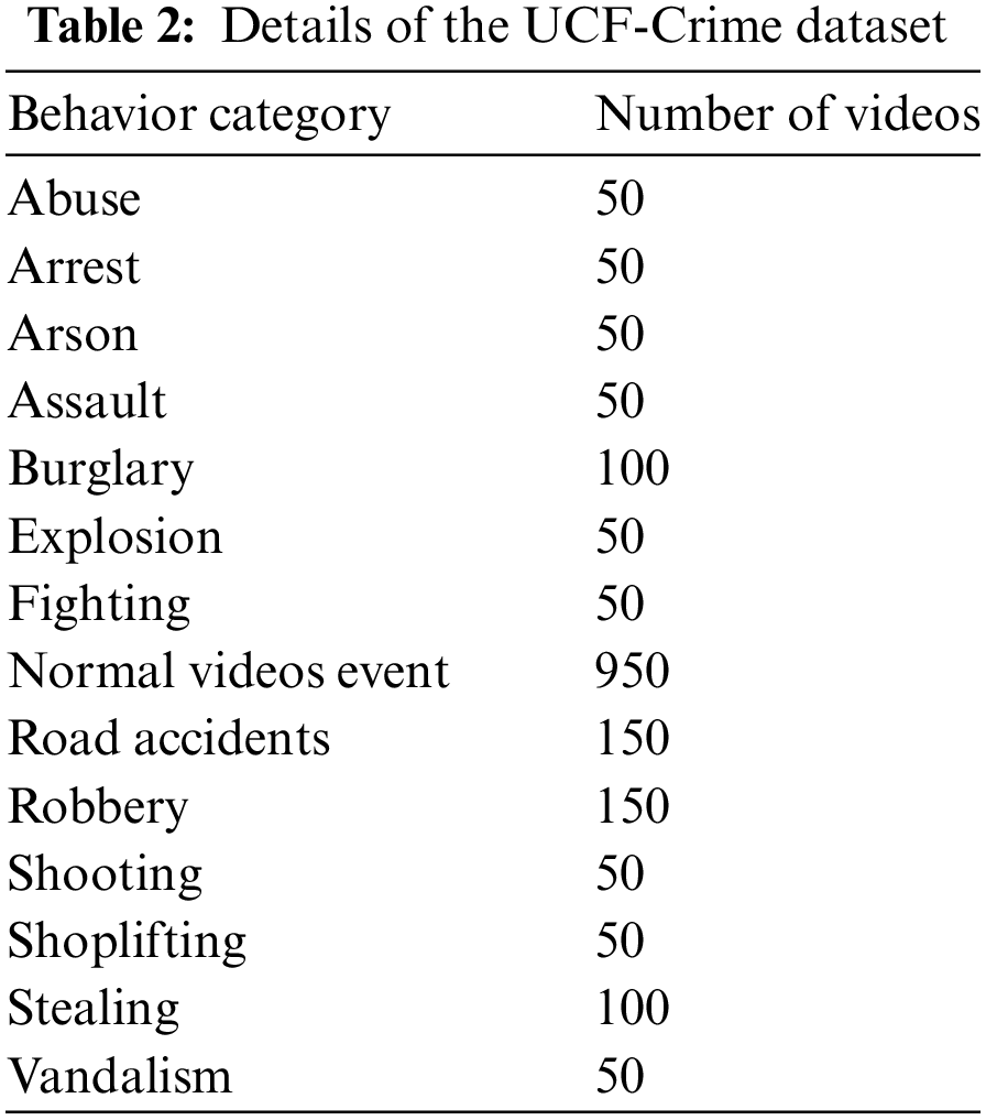
We used the large abnormal behavior dataset UCF-Crime for training and testing, which contains many categories of abnormal behavior videos and a large number of normal videos. The types of abnormal behaviors include arrest, arson, stealing, road accidents, etc. The specific data are shown in Table 2. The dataset contains a total of 1900 surveillance video data. All experiments were conducted on an Intel Xeon CPU and a 2080Ti GPU.

The UCF-Crime dataset is a large video dataset aimed for research in anomalous event detection. This dataset contains real-world surveillance videos, covering a wide variety of criminal and anomalous behaviors, including various unusual vehicular activities such as cargo scattering, vehicle combustion, vehicle collisions, etc. In our study, we extract videos related to unusual vehicular behaviors to create a new video dataset, utilizing this new dataset to conduct research on the detection of unusual vehicular activities. In order to avoid the influence of manual editing on the training results, the videos in the dataset are screened so that all the videos in the dataset are unedited. In this dataset, there are 150 videos with serious traffic abnormal behaviors and 950 normal videos without abnormal behaviors, as shown in Fig. 7.

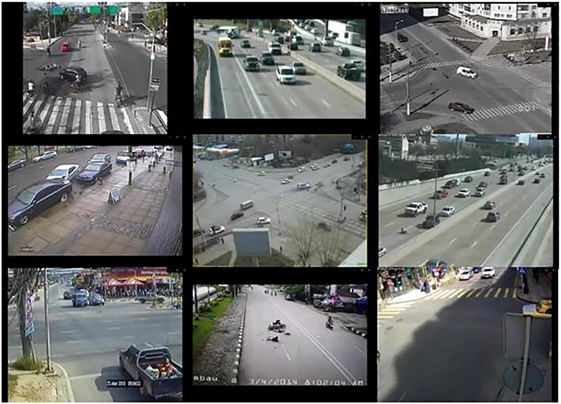
Figure 7: Sampling images with the dataset

To compare our models with other models, we constructed six models and compared them experimentally. They are R3D, R3D + LSTM, R3D + Bi-LSTM, DRN, DRN + LSTM, and DRN + Bi-LSTM. The vehicle’s abnormal behavior detection can be seen as a dichotomous problem, so we use the dichotomous accuracy formula as an evaluation criterion, as shown in Eq. (8).

Accuracy=Tp+TnTp+Tn+Fp+Fn(8)

where Tp is the positive sample that is predicted to be positive by the model, Tn is the negative sample that is predicted to be negative by the model, Fp is the negative sample that is predicted to be positive by the model, Fn is the positive sample that is predicted to be negative by the model.

The accuracy of our model on the training and validation sets is shown in Fig. 8. From the figure, we can see that the recognition accuracy gradually increases in the first 15 epochs, and then tends to level off. Moreover, after 10 epochs, the difference in accuracy between the training and validation sets is not significant, indicating that our model does not appear to be over-fitted and the model has good generalization ability.

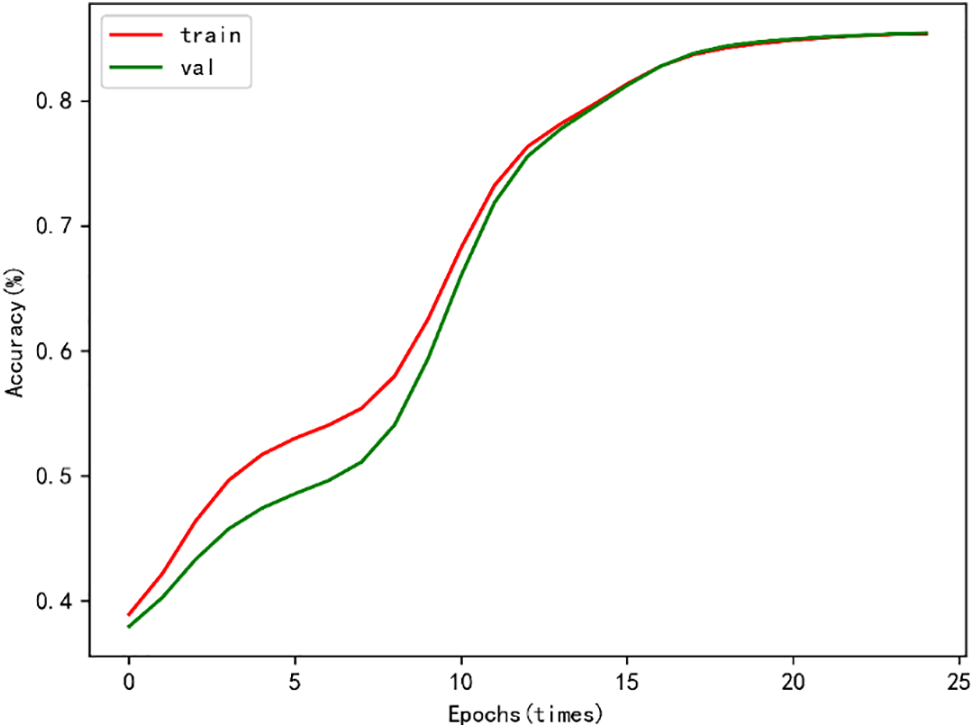
Figure 8: Accuracy of DRN + Bi-LSTM on the training set and validation set

To compare the recognition accuracy of the different models, we used the six models mentioned above to train, validate and test in the same environment. The training process consisted of 25 epochs, all with an initial learning rate of 0.01. The learning rate decreased by a factor of 10 after every 5 epochs. Each epoch outputs the current recognition accuracy, and the experimental results are shown in Fig. 9.

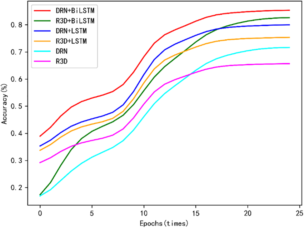
Figure 9: Accuracy of each model on the test set

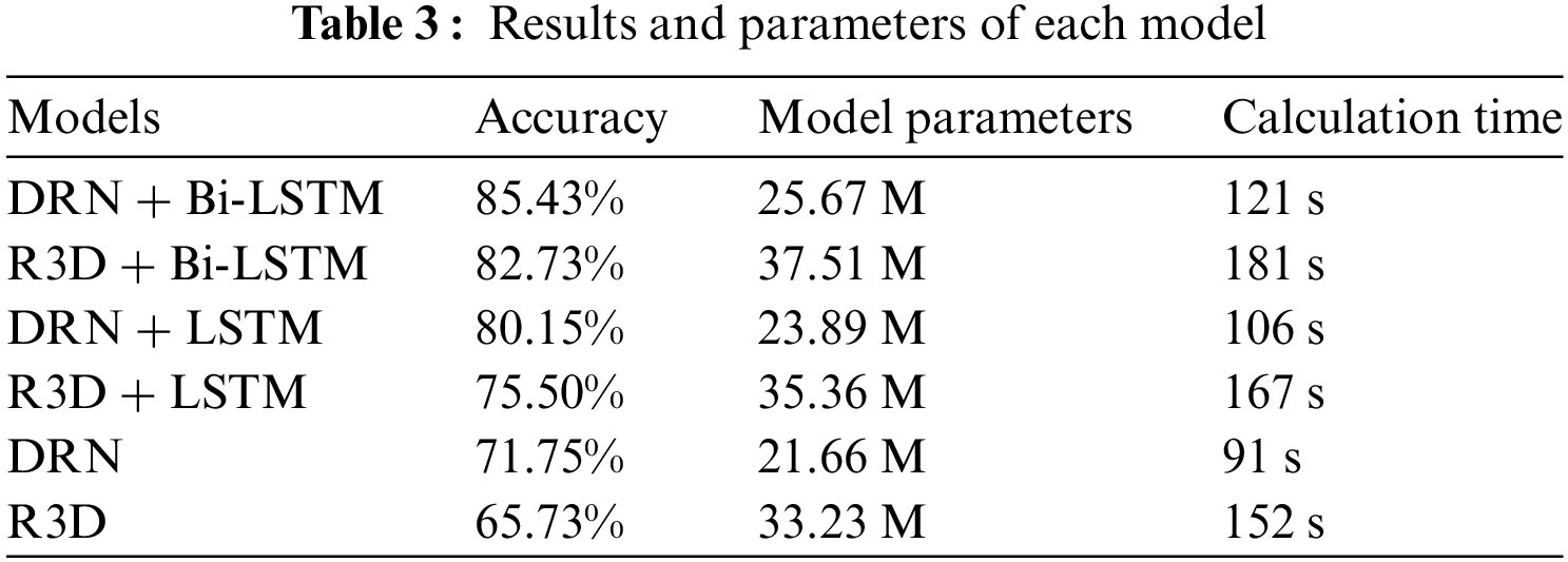
The final experimental results are shown in Table 3. From the table, we can see that the recognition accuracy of the R3D on the UCF-Crime dataset is not high, only 65.73%. In contrast, the DRN + Bi-LSTM has the highest recognition accuracy of 85.43% in the same environment. Moreover, compared with the R3D, the DRN has fewer model parameters, shorter computation time and higher efficiency.

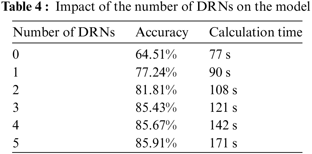
In order to verify the effect of the number of DRNs in our model, we designed an ablation experiment to see the performance of the model by increasing or decreasing the number of DRN modules in the model. The results are shown in Table 4. It can be seen that as the number of DRN modules in the model increases, the recognition rate of the model is also increasing. However, it can be seen that when the number of DRN modules is greater than 3, the model’s recognition accuracy improves to a limited extent and the computation time increases significantly. Therefore, taking into account the overall consideration and balancing the recognition accuracy and computational efficiency of the model, we add 3 DRN modules to the model.

To further evaluate the accuracy of the above models in vehicle abnormal behavior detection, different abnormal behaviors in the dataset were used separately for experimental comparison. The aberrant behavior labels in the test set include arrest, arson, burglary, road accidents, robbery, shoplifting, and vandalism. We recorded the recognition accuracy of each model in different datasets separately, as shown in Table 5. As we can see from the table, all six models are not suitable for detecting some abnormal behaviors, such as arrest and shoplifting, but perform well in road accident detection. Among them, DRN + Bi-LSTM has the best recognition result with 89.30%. This suggests that our model is better suited for the identification and detection of abnormal vehicle behavior.

To evaluate the performance of our models (Dense Block and Soft Thresholding for the local feature extraction network and the Bi-LSTM for the global feature extraction network), we conducted a comparison experiment with good feature extraction networks (P3D, I3D, and R(2 + 1)D) on the test set. The experimental result is shown in Fig. 10.

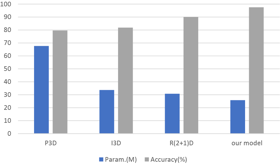
Figure 10: Comparison of parameter overhead and accuracy

5  Conclusion

To sum up, for the network proposed in this paper, we first use 3D convolution and maximum pooling to reduce the size of the feature map, expand the perceptual domain, and reduce the number of parameters. Then, we use DRN blocks to improve the feature utilization of the network and improve the computational efficiency. This makes it easier to train the network without adding additional calculations. To solve the overfitting problem, we use Dropout and soft thresholds to remove noise and adjust the features we need. Finally, Bi-LSTM is used to further enhance the time feature extraction. Experimental results show that the model can improve the recognition accuracy of UCF-crime data set. This model is more suitable for the recognition of vehicle abnormal behavior. The simulation of the actual application is shown in Fig. 11, where “Frames” in the coordinate axis represents the number of frames in a video, and “Score” indicates the anomaly score. The higher anomaly score indicates a higher probability of abnormal vehicle behavior in the current frame. As can be seen from the figure, our model can accurately detect the time when the abnormal behavior of the vehicle occurs. If the exception does not disappear, the model continues to judge the situation as an exception. Only when the abnormal behavior disappears does the model judge that the situation is normal at that time. The experiment proves that the model can be integrated into the intelligent traffic management system, improve the accuracy, timeliness, and efficiency of traffic monitoring.

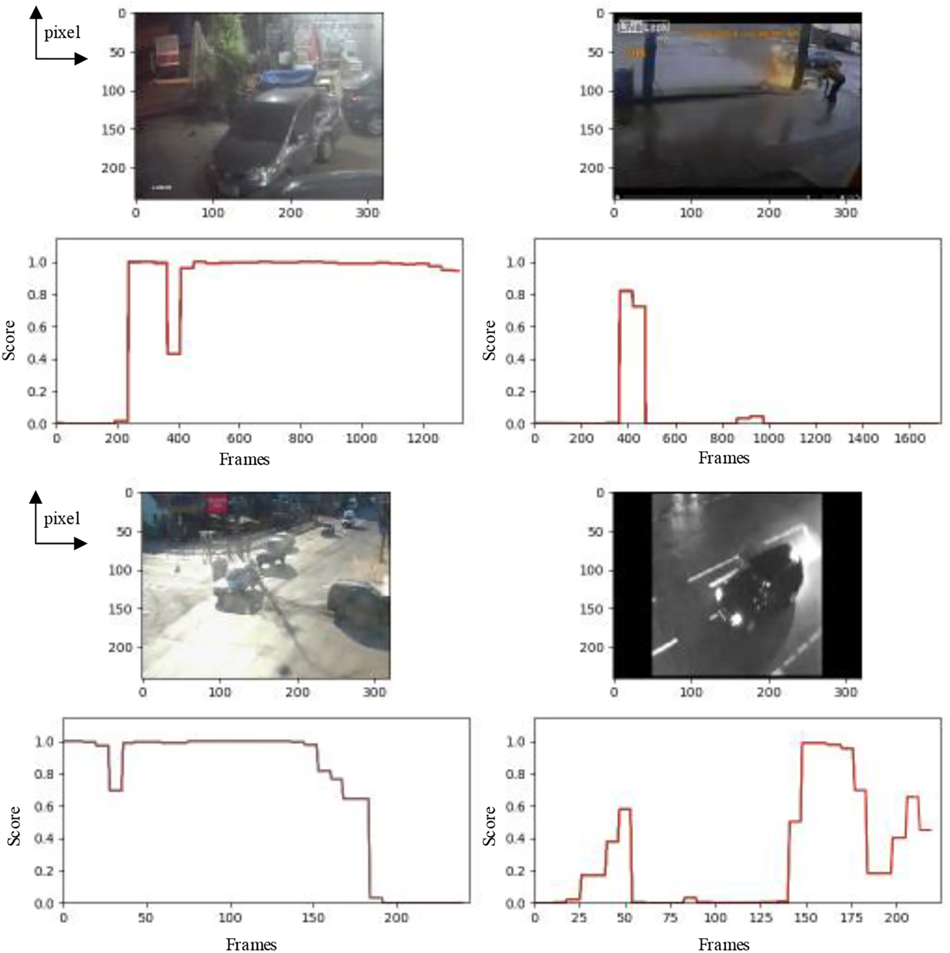
Figure 11: Simulation of applications

Acknowledgement: The authors wish to thank the National Natural Science Foundation of China and the North China University of Technology for the vital support provided for this research. All authors are thankful to the editor, Ramey Jue, and all the anonymous reviewers for their suggestions which have contributed to enhancing the quality of the manuscript.

Funding Statement: This work was supported by the National Natural Science Foundation of China (61971007 & 61571013).

Author Contributions: Study conception and design: Wei Chen, Yuanyao Lu, Zhanhe Yu; data collection: Chaochao Yang; analysis and interpretation of results: Zhanhe Yu, Jingxuan Wang; draft manuscript preparation: Zhanhe Yu, Chaochao Yang. All authors reviewed the results and approved the final version of the manuscript.

Availability of Data and Materials: Data available on request from the authors.

Conflicts of Interest: The authors declare that they have no conflicts of interest to report regarding the present study.

References

1. L. Zhu, F. R. Yu, Y. Wang, B. Ning, and T. Tang, “Big data analytics in intelligent transportation systems: A survey,” IEEE Trans. Intell. Transp. Syst., vol. 20, no. 1, pp. 383–398, Jan. 2019. doi: 10.1109/TITS.2018.2815678. [Google Scholar] [CrossRef]

2. M. Veres and M. Moussa, “Deep learning for intelligent transportation systems: A survey of emerging trends,” IEEE Trans. Intell. Transp. Syst., vol. 21, no. 8, pp. 3152–3168, Aug. 2020. doi: 10.1109/TITS.2019.2929020. [Google Scholar] [CrossRef]

3. F. Zhu, Y. Lv, Y. Chen, X. Wang, G. Xiong and F. Y. Wang, “Parallel transportation systems: Toward IoT-enabled smart urban traffic control and management,” IEEE Trans. Intell. Transp. Syst., vol. 21, no. 10, pp. 4063–4071, Oct. 2020. doi: 10.1109/TITS.2019.2934991. [Google Scholar] [CrossRef]

4. Y. Ren, Z. Lan, L. Liu, and H. Yu, “EMSIN: Enhanced multi-stream interaction network for vehicle trajectory prediction,” IEEE Trans. Fuzzy Syst., pp. 1–15, 2024. doi: 10.1109/TFUZZ.2024.3360946. [Google Scholar] [CrossRef]

5. W. Huang, X. Liu, M. Luo, P. Zhang, W. Wang, and J. Wang, “Video-based abnormal driving behavior detection via deep learning fusions,” IEEE Access, vol. 7, pp. 64571–64582, 2019. doi: 10.1109/ACCESS.2019.2917213. [Google Scholar] [CrossRef]

6. J. Hu, L. Xu, X. He, and W. Meng, “Abnormal driving detection based on normalized driving behavior,” IEEE Trans. Veh. Technol., vol. 66, no. 8, pp. 6645–6652, Aug. 2017. doi: 10.1109/TVT.2017.2660497. [Google Scholar] [CrossRef]

7. H. F. Sang, H. Wang, and D. Y. Wu, “Vehicle abnormal behavior detection system based on video,” in Proc. 2012 Fifth Int. Symp. Comput. Intell. Design, Hangzhou, China, 2012, pp. 132–135. doi: 10.1109/ISCID.2012.41. [Google Scholar] [CrossRef]

8. J. Hu, X. Zhang, and S. Maybank, “Abnormal driving detection with normalized driving behavior data: A deep learning approach,” IEEE Trans. Veh. Technol., vol. 69, no. 7, pp. 6943–6951, Jul. 2020. doi: 10.1109/TVT.2020.2993247. [Google Scholar] [CrossRef]

9. S. Liang et al., “Fiber-optic auditory nerve of ground in the suburb: For traffic flow monitoring,” IEEE Access, vol. 7, pp. 166704–166710, 2019. doi: 10.1109/ACCESS.2019.2952999. [Google Scholar] [CrossRef]

10. Z. Luo, M. V. Mohrenschildt, and S. Habibi, “A probability occupancy grid based approach for real-time LiDAR ground segmentation,” IEEE Trans. Intell. Transp. Syst., vol. 21, no. 3, pp. 998–1010, Mar. 2020. doi: 10.1109/TITS.2019.2900548. [Google Scholar] [CrossRef]

11. Y. Li et al., “Multi-granularity tracking with modularlized components for unsupervised vehicles anomaly detection,” in Proc. 2020 IEEE/CVF Conf. Comput. Vis. Pattern Recognit. Workshops (CVPRW), Seattle, WA, USA, 2020, pp. 2501–2510. doi: 10.1109/CVPRW50498.2020.00301. [Google Scholar] [CrossRef]

12. Q. Hao and L. Qin, “The design of intelligent transportation video processing system in big data environment,” IEEE Access, vol. 8, pp. 13769–13780, 2020. doi: 10.1109/ACCESS.2020.2964314. [Google Scholar] [CrossRef]

13. S. Wan, X. Xu, T. Wang, and Z. Gu, “An intelligent video analysis method for abnormal event detection in intelligent transportation systems,” IEEE Trans. Intell. Transp. Syst., vol. 22, no. 7, pp. 4487–4495, Jul. 2021. doi: 10.1109/TITS.2020.3017505. [Google Scholar] [CrossRef]

14. J. Wang, X. Li, S. S. Liao, and Z. Hua, “A hybrid approach for automatic incident detection,” IEEE Trans. Intell. Transp. Syst., vol. 14, no. 3, pp. 1176–1185, Sep. 2013. doi: 10.1109/TITS.2013.2255594. [Google Scholar] [CrossRef]

15. K. Zhang and M. A. P. Taylor, “Effective arterial road incident detection: A bayesian network based algorithm,” Transp Res. C, Emerg. Technol., vol. 14, no. 6, pp. 403–417, Dec. 2006. doi: 10.1016/j.trc.2006.11.001. [Google Scholar] [CrossRef]

16. Q. Liu, J. Lu, S. Chen, and K. Zhao, “Multiple Naïve Bayes classifiers ensemble for traffic incident detection,” Math. Problems Eng., vol. 2014, pp. 1–16, Apr. 2014. [Google Scholar]

17. L. Li, Y. Lin, B. Du, F. Yang, and B. Ran, “Real-time traffic incident detection based on a hybrid deep learning model,” Transportmetrica A, vol. 18, no. 1, pp. 78–98, 2020. doi: 10.1080/23249935.2020.1813214. [Google Scholar] [CrossRef]

18. S. Li, J. Chen, W. Peng, X. Shi, and W. Bu, “A vehicle detection method based on disparity segmentation,” Multimed. Tools Appl., vol. 82, no. 13, pp. 19643–19655, 2023. doi: 10.1007/s11042-023-14360-x. [Google Scholar] [CrossRef]

19. H. Zhang, G. Luo, J. Li, and F. Wang, “C2FDA: Coarse-to-fine domain adaptation for traffic object detection,” IEEE Trans. Intell. Transp. Syst., vol. 23, no. 8, pp. 12633–12647, Aug. 2022. doi: 10.1109/TITS.2021.3115823. [Google Scholar] [CrossRef]

20. K. He, X. Zhang, S. Ren, and J. Sun, “Deep residual learning for image recognition,” in Proc. 2016 IEEE Conf. Comput. Vis. Pattern Recognit. (CVPR), Las Vegas, NV, USA, 2016, pp. 770–778. doi: 10.1109/CVPR.2016.90. [Google Scholar] [CrossRef]

21. Y. Ibrahim et al., “Soft error resilience of deep residual networks for object recognition,” IEEE Access, vol. 8, pp. 19490–19503, 2020. doi: 10.1109/ACCESS.2020.2968129. [Google Scholar] [CrossRef]

22. G. Huang, Z. Liu, L. van der Maaten, and K. Q. Weinberger, “Densely connected convolutional networks,” in Proc. 2017 IEEE Conf. Comput. Vis. Pattern Recognit. (CVPR), Honolulu, HI, USA, 2017, pp. 2261–2269. doi: 10.1109/CVPR.2017.243. [Google Scholar] [CrossRef]

23. T. Li, W. Jiao, L. N. Wang, and G. Zhong, “Automatic DenseNet sparsification,” IEEE Access, vol. 8, pp. 62561–62571, 2020. doi: 10.1109/ACCESS.2020.2984130. [Google Scholar] [CrossRef]

24. S. Zhai, D. Shang, S. Wang, and S. Dong, “DF-SSD: An improved SSD object detection algorithm based on DenseNet and feature fusion,” IEEE Access, vol. 8, pp. 24344–24357, 2020. doi: 10.1109/ACCESS.2020.2971026. [Google Scholar] [CrossRef]

25. L. Yuan, F. E. H. Tay, P. Li, and J. Feng, “Unsupervised video summarization with cycle-consistent adversarial LSTM networks,” IEEE Trans. Multimed., vol. 22, no. 10, pp. 2711–2722, Oct. 2020. doi: 10.1109/TMM.2019.2959451. [Google Scholar] [CrossRef]

26. E. Ahmadzadeh, H. Kim, O. Jeong, N. Kim, and I. Moon, “A deep bidirectional LSTM-GRU network model for automated ciphertext classification,” IEEE Access, vol. 10, pp. 3228–3237, 2022. doi: 10.1109/ACCESS.2022.3140342. [Google Scholar] [CrossRef]

27. P. Limcharoen, N. Khamsemanan, and C. Nattee, “Gait recognition and re-identification based on regional LSTM for 2-second walks,” IEEE Access, vol. 9, pp. 112057–112068, 2021. doi: 10.1109/ACCESS.2021.3102936. [Google Scholar] [CrossRef]

28. R. Zhong, R. Wang, Y. Zou, Z. Hong, and M. Hu, “Graph attention networks adjusted Bi-LSTM for video summarization,” IEEE Signal Process. Lett., vol. 28, pp. 663–667, 2021. doi: 10.1109/LSP.2021.3066349. [Google Scholar] [CrossRef]

29. H. Zhang, S. Sun, Y. Hu, J. Liu, and Y. Guo, “Sentiment classification for chinese text based on interactive multitask learning,” IEEE Access, vol. 8, pp. 129626–129635, 2020. doi: 10.1109/ACCESS.2020.3007889. [Google Scholar] [CrossRef]

30. M. Alizadeh and J. Ma, “High-dimensional time series analysis and anomaly detection: A case study of vehicle behavior modeling and unhealthy state detection,” Adv Eng. Informatics., vol. 57, no. 1, pp. 102041, 2023. doi: 10.1016/j.aei.2023.102041. [Google Scholar] [CrossRef]