Exploring Motor Imagery EEG: Enhanced EEG Microstate Analysis with GMD-Driven Density Canopy Method

1  Introduction

Advancements in neuroscience continue to deepen our understanding of brain activity. EEG as a non-invasive tool for recording brain physiological activity, is widely applied in the analysis of brain functional states and clinical disease research, such as stroke [1], epilepsy [2], Alzheimer’s disease [3], among others. Additionally, EEG forms the cornerstone of brain function and Brain-Computer Interface (BCI) studies, capturing the intricate spatiotemporal dynamic processes of the cerebral cortex.

Within the range of diverse BCI paradigms, Motor Imagery-based BCI (MI-BCI) has consistently captivated researchers. This technological paradigm enables subjects to engage with external devices through imagining a specific movement (e.g, hand or foot movements) [4,5], offering a potential avenue for interaction among individuals with disabilities and a novel prospects for rehabilitation therapy. Nevertheless, motor imagery EEG signals exhibit complexity and variability, necessitating advanced signal processing and analysis methods to comprehensively grasp their underlying mechanisms and enhance the performance of MI-BCI. Conventional signal processing methods for MI-BCI include time frequency eigen analysis [6,7], autoregression [8], co-spatial patterns [9], empirical modal decomposition [10], traceability analysis [11], and Riemannian geometry [12], among others. Although these methods can be effective in some scenarios to process the EEG signals, they may not be able to adequately capture the features of the signals in some applications due to the nonlinearity and complexity of the EEG signals. Therefore, in recent years, deep learning algorithms have been integrated with MI-BCI, and Altaheri et al. [13] analyzed the deep learning-based motor imagery classification technique in detail from four aspects. The results of the analysis show that deep learning algorithms still perform well in processing EEG data with low channel counts and without band filtering. Also the Convolutional Neural Network (CNN) based deep learning network performs best when using topological images as input. Although deep learning algorithms show excellent performance in classifying motor imagery datasets, they are unable to peek into the internal logic of their decision-making process, making it difficult to gain a deeper understanding of the complex mechanisms of brain activity during motor imagery. Therefore, we need a method that can directly capture and parse changes in brain dynamics and provide intuitive and easy-to-understand results for in-depth research.

Microstate analysis serves as a method to characterize the spatiotemporal dynamics of large-scale electrophysiological signals and is regarded as the ‘thought atom’ of the human mind [14]. Emphasizing microstates in EEG signals, this approach offers more nuanced insights. Wu et al. [15] applied microstate analysis to the study of attention deficit and found that the duration of microstate C in patients increased, while its classification accuracy reached 93.59%. Chu et al. [16] analyzed the temporal and spatial variability of brain network in Parkinson’s disease, and its classification accuracy reached 95.69%. Luo et al. [17] applied microstate analysis to the prediction of schizophrenia and achieved an average classification accuracy of 92% for its four groups. Conventional microstate analysis methods commonly partition resting EEG data from healthy subjects into four standard microstate topographies [18,19]. Nevertheless, the clustering of EEG data into only four microstates may not sufficiently capture the complex and diverse information inherent in the EEG signal. Research findings indicate that EEG signals typically encompass multiple microstates, each potentially reflecting distinct brain activities, including visual processing, language comprehension, emotions, etc. [20]. Reducing the microstates in EEG to only four may lead to a loss of valuable EEG information [21]. Due to the complexity of motor imagery tasks, it is needed to precisely divide the microstate clusters with some margin to accommodate inter-individual variability.

For the traditional microstate analysis method K-means clustering is employed to ascertain the number of microstate clusters [22,23]. The K-means algorithm, a frequently employed partitional clustering algorithm [24–26], is known for its simplicity and efficiency, rendering it suitable for cluster analysis of large datasets. Nevertheless, the K-means clustering algorithm encounters two specific challenges, namely, establishing the number of clusters (K value) and choosing the initial cluster center [27]. A method proposed in related research [28] to ascertain the input parameters for clustering by combining the canopy algorithm with the K-means algorithm to reduce resistance to interference. Zhang et al. [29] extended previous research by proposing a clustering algorithm utilizing density canopy within the framework of the K-means method. Determining both the number of microstate clusters and the initial clustering center through calculations involving sample density and the maximum weight method are determined. Subsequently, these results are utilized as the initial values for the K-means algorithm. Nevertheless, this algorithm exhibits suboptimal performance in processing high-dimensional data and is not applicable to the processing of high-dimensional EEG signals.

Hence, for a more efficient processing of EEG signals, This study introduces an enhanced K-means clustering algorithm. The algorithm has lower computational cost as well as stronger robustness. The main contributions of this study are categorized into the following three areas. 1) We propose a clustering algorithm that automatically determines the optimal number of microstates, overcoming the limitations of traditional methods. 2) By optimizing and improving the algorithm, we make it more adaptable to the characteristics of high-dimensional data, so that it can extract and analyze microstate information in EEG signals more effectively. 3) Our proposed method has made significant improvements in cross-task feature extraction, obtaining more accurate and robust results. Specifically speaking, initially, the kernel density estimation with a Gaussian kernel function is employed to model the data and precisely evaluate the initial density of the samples. Subsequently, the determination of sample points within the cluster is based on the GMD of the microstate topography map. Furthermore, the introduction of average distance and isolation within the cluster aims to strike a balance between tightness within the cluster and separation between clusters during the clustering process. This ensures accurate classification of each sample, allowing for better capturing of key information in EEG signals. Ultimately, the optimal number of microstates is automatically determined through the Maximum Weighting Method. Finally, the algorithm presented in this paper is applied to model and analyze motor imagery EEG data. The experimental findings indicate the superior performance of the proposed algorithm over traditional clustering methods, leading to a substantial improvement in the accuracy of motor imagery classification tasks.

The paper follows this structure: Section 1 introduces the experimental data and Outlines an enhanced K-means clustering algorithm for dense canopy that includes GMD drivers; Section 2 presents the experimental results; while Sections 3 and 4 discuss the results obtained from the experiments and draw conclusions, respectively.

2  Data and Methods

2.1 Data Sources and Preprocessing

The experimental data for this study were sourced from the GigaScience database (http://dx.doi.org/10.5524/100295). This dataset recorded a total of 52 motor imagery EEG datasets from healthy subjects, and 20 real hand movement EEG datasets. The acquisition equipment utilized 64 Ag/AgCl active electrodes for collecting EEG data, following the international 10-10 system standard arrangement. The experimental process unfolded as follows: At the experiment’s initiation, the monitor displayed a black screen, with the participants fixing their gaze for two seconds. Subsequently, subjects prepared for either actual hand movement or imagined hand movement (indicated by a clear signal on the screen). Following this, the screen displayed one of the two commands, “left hand” or “right hand”. Following this, one of the two commands, either “left hand” or “right hand” appeared on the screen, and after 3 s, the screen went blank. Data preprocessing was carried out using the EEGLAB toolbox in Matlab. Initially, Independent Component Analysis (ICA) was applied to identify and eliminate artifacts stemming from eye, heart, and muscle activities. Subsequently, band-pass filtering was implemented using a Finite Impulse Response (FIR) filter within the frequency range of 1–40 Hz, followed by average reference. Finally, the preprocessed dataset was divided into 3-s segments for subsequent data analysis.

2.2 EEG Microstate Analysis

Microstate analysis can be viewed as a dimensionality reduction technique that aims to reduce each microstate into a one-dimensional subspace. The general process of microstate analysis is as follows:

Initially, to capture information about the overall amplitude of the EEG data and its activity level, it is imperative to compute the Global Field Power (GFP). GFP signifies the spatial standard deviation of the instantaneous EEG data at time point i, providing a metric that characterizes the intensity of the topographic map at each time point, irrespective of the reference electrode selection. The calculation formula is as follows (1):

GFPt=∑Ni=1[Vi(t)−V(t)¯]2N(1)

where N is the number of electrodes, Vi(t) is the voltage value of the ith electrode at moment t, and V(t) is the average voltage value of all electrodes at moment t.

Through the above calculations, a GFP curve reflecting the degree of change in the EEG potential between all electrodes at a given time is obtained. Since the local maxima of the GFP curves have the strongest signal strength and the highest signal-to-noise ratio, the topographic maps at the local maxima of the GFP were selected for subsequent cluster analysis. Initially, individualized microstate analysis was conducted on the EEG data of each subject. For each subject, the local maxima of the GFP curves were employed as inputs into a modified density canopy K-means clustering algorithm for the initial clustering. Following the acquisition of initial clustering results, a secondary clustering analysis was conducted to delve deeper into the microstates across the entire dataset.

2.3 Density Canopy K-Means Clustering Algorithm Driven by GMD

2.3.1 Canopy Algorithm

The Canopy algorithm is frequently utilized as a preliminary step for either the K-means algorithm. The crux of the Canopy algorithm lies in setting two distance thresholds, T1 and T2 (where T1 > T2), and creating a canopy based on them. The assignment of clusters to which the sample points belong is performed by randomizing the initial cluster centers and calculating the Euclidean distance between the sample points.

The objective of these steps is to generate a series of disjoint canopies, where each canopy comprises a set of sample points with distances between T1 and T2 from the initial clustering center. These canopies can be regarded as initial clusters, subject to further refinement or merging in subsequent clustering processes, ultimately yielding the final clustering results. Notably, the primary advantage of the Canopy algorithm lies in its effective reduction of data dimensionality, thereby diminishing the computational complexity of subsequent clustering algorithms.

Despite the Canopy algorithm plays a crucial role in facilitating the initialization of cluster centers for the K-means algorithm, it requires manual determination of the thresholds, T1 and T2. The careful selection of these thresholds significantly influences clustering performance. If T1 and T2 are set too large, there is a risk of incorrectly merging data points belonging to different classes into the same cluster, thereby compromising the accuracy of the clustering. Conversely, if these thresholds are set too small, there is a possibility of data points belonging to the same class being split into multiple unnecessarily small clusters, resulting in overly refined clustering outcomes.

2.3.2 GMD-Driven Density Canopy Clustering Algorithm

Given that the initial clustering center selection in the Canopy algorithm is random, which directly impacts the final clustering results. Hence, the selection of the initial clustering center can be based on the density of the sample points. This method involves the utilization of a Gaussian kernel function, the formula for which is illustrated in Eq. (2).

K(xi,xj)=exp(−d(xi,xj)22σ2)(2)

where d represents the Euclidean distance between two points, and σ serves as a control parameter influencing the density of the kernel function, acting as a bandwidth parameter.

Place the kernel function at the location of each sample point, and the kernel density between it and the other data points is calculated using the chosen kernel function. The density formula is provided below:

KDE(xi)=1n∑j=1nK(xi,xj)(3)

Each kernel function is centered on its respective data point, resulting in a copy of the kernel function for each data point. Through these copies, local density estimates are constructed at different sample points. Then, stack all copies of the kernel function together to form a density estimate for the entire dataset, capturing local density information at different positions in the dataset. Finally, the density estimate is normalized to ensure that it constitutes a legitimate probability density function. And selected the sample point with the highest density as the initial clustering center.

Simultaneously, recognizing the significant impact of manually setting the threshold in the Canopy algorithm on clustering results, the maximum weight method is introduced to enhance the accuracy of the clustering algorithm. The following outlines the fundamental concepts utilized in the algorithm.

Definition 1: The GMD index between sample points is defined as:

GDM=1N∑i=1N(ui−u¯GFPu−vi−v¯GFPv)2(4)

Definition 2: Define the average distance of the samples in dataset D as:

meandis(D)=2n(n−1)∑i=1n∑j=i+1nd(xi,xj)(5)

Definition 3: Define the number of sample points in the dataset that belong to the same cluster as sample point i as:

num(i)=∑j=1nf(dij−meandis(D)),f(x)={1,x<00,x>0(6)

Definition 4: According to the formula in Definition 2, define a(i) as the average distance of the sample points within the cluster to which sample point i belongs, calculated among the remaining sample points:

a(i)=2num(i)[num(i)−1]∑i=1num(i)∑j=i+1num(i)d(xi,xj)(7)

Definition 5: If sample point i is the one with the largest density value (the peak sample), s(i) is equal to the maximum value of the distance from i within the distance matrix, serving as an indicator of the isolation of the peak sample. If sample point i is not the peak sample, the smallest of these distances is returned.

Definition 6: Define the weight of sample point i as the product of the density of sample point i, the inverse of a(i) and s(i):

w=ρ(i)∗1a(i)∗s(i)(8)

where ρ(i) is the density value of sample point i, a(i) is the average distance among the remaining samples, and s(i) is the isolation of the sample point.

Introducing kernel function density estimation along with the maximum weight method in the Canopy algorithm enables the automatic determination of the optimal number of microstate clusters, eliminating the need for manual adjustment of the threshold. This enables the algorithm to adapt to different datasets and improves the robustness of the algorithm. In the improved algorithm, firstly, the density matrix is calculated by kernel function density estimation, and then the sample point i with the highest density is selected as the first initial clustering centre according to the density matrix. Simultaneously, the GMD index between the initial clustering center and the remaining sample points is calculated according to Eq. (4). Eligible sample points are merged into the cluster corresponding to this clustering center, which is subsequently excluded from the dataset. Following that, the weight values of the remaining sample points are calculated according to Eq. (8). The sample point with the largest weight value is then selected as the second initial clustering center. Iterate through the previously mentioned steps until the dataset is depleted. This algorithm has demonstrated its efficacy in filtering out outlier data, as outlier points commonly display distinct and low density. Thus, during the calculation of the maximum weight method, if ρ(i) is smaller and s(i) is larger, it indicates an outlier point. Consequently, such points are eliminated.

The flow of the improved algorithm is depicted in Algorithm 1. The following provides an overview of the approximate steps in the algorithm implementation:

Step 1: Estimate the density of all sample points by kernel function estimation density, and then select the sample point i with the highest density according to the density matrix, and add it to the clustering set CANOPY. And then calculate the GMD index between sample point i and the rest of the sample points, classify the sample points that meet the conditions into the cluster where sample point i is located, and exclude the cluster.

Step 2: Calculate a(i) and s(i). Find the w value of each sample point according to Eq. (8). Determine the second cluster centre and place it in the CANOPY list. Similarly perform operations such as deleting clusters.

Step 3: Repeat step 2 until the dataset D is empty. And get the initial clustering centre list CANOPY.

Step 4: The initial clustering centres obtained are used as input to the K-means algorithm for K-means clustering:

The flow of the algorithm is shown in Fig. 1:

Figure 1: Flow chart of GMD-driven density canopy K-means algorithm

2.4 Microstate Characteristic Parameters

After obtaining the microstate sequence, the following microstate parameters can be calculated:

Mean Duration: The average duration length of the microstate in the EEG data, reflecting the temporal characteristics of the microstate.

Frequency: The frequency or occurrence rate of microstates appearing in EEG data, reflecting the frequency characteristics of microstates.

Repetition Time Ratio: The ratio of the total time a microstate occurs to the total duration of a time series, representing the repeatability or persistence of the microstate.

2.5 Dynamic Attributes of Microstate Sequences

To offer a more thorough description and comprehension of EEG activity. In order to quantify the complexity, regularity, the dynamic properties of microstate sequences, Shannon entropy, entropy rate, sample entropy, and Lempel-Ziv complexity are employed to measure the dynamic parameters of microstate sequences.

2.5.1 Shannon Entropy

Shannon Entropy: Shannon entropy is a concept in information theory used to measure the uncertainty or randomness of signals or data. In EEG signal analysis, Shannon entropy is often used to describe the complexity of EEG signals. Shannon entropy can be used to reveal the complexity and informativeness of EEG signals and provide important clues for understanding the variability and dynamics of EEG activity. The formula for Shannon entropy is:

Ent(D)=−∑i=1np(xi)log2⁡p(xi)(9)

2.5.2 Entropy Rate

Entropy Rate: Entropy rate is a measure of the dynamic complexity of a signal, reflecting the rate of change of information in the signal. In EEG signal analysis, entropy rate is often used to describe the rapid changes and dynamics of EEG signals. The entropy rate can indicate how fast the information in the signal changes. The calculation of entropy rate can be based on the change in entropy value of the signal over time to assess the dynamic complexity of the signal. The entropy rate is calculated by the formula:

H(χ)=limn→∞1nH(X1,X2,…,Xn)(10)

2.5.3 Sample Entropy

Sample Entropy: Sample Entropy is a metric used to quantify the complexity and regularity of a signal. Similar to Shannon entropy, sample entropy is used to measure the uncertainty or randomness of a signal. Unlike Shannon entropy, sample entropy also takes into account the self-similarity of the signal. The calculation of sample entropy can be used to assess the regularity of a signal based on its repeated patterns and similarities.

2.5.4 Lempel Ziv Complexity

Lempel Ziv Complexity (LZC) [30,31]: LZC is defined as the number of distinct subsequences in a left-to-right sequence. A string is considered to have low LZC if it exhibits a small number of frequently repeated sequences. Thus, the sequences with low LZC are repetitive. Conversely, high LZC implies that the sequence has high complexity. In this paper, LZC is applied to EEG microstate sequences. C(N) represents the number of distinct substrings included in the sequence, reflecting the number of new patterns in the sequence.

c(N)≺N(1−δN)logα⁡N(11)

where c(N) is the absolute complexity of the time series, N is the length of the microstate sequence (number of time samples), and α is the number of distinct subsequences in the time series. δN is a very small quantity, and as N approaches infinity, δN tends to 0.

limn→∞c(N)=bN=Nlogα⁡N(12)

To mitigate the impact of varying sequence lengths on complexity, c(N) is typically normalized to create the relative complexity, C(N). The calculation of C(N) is as follows:

C(N)=c(N)b(N)(13)

b(N)=Nlog⁡2N(14)

where b(N) represents the asymptotic behavior of the time series, implying that sequences within the interval [0,1] converge to a fixed upper bound as the length of the sequence becomes sufficiently long.

3  Results

3.1 Microstate Topographic Map

For the motion imagery dataset, we applied a modified density canopy-based K-means clustering algorithm to extract microstate topographic maps. Various numbers of microstate topographies were extracted for different tasks. For left-handed imagined motion, five microstates explained 72.64% of the data in the global field power peak; for left-handed actual motion, five microstates explained 76.20% of the data; for right-handed imagined motion, five microstates explained 75.96% of the data; and for right-handed actual motion, six microstates explained 73.87% of the data. The specific microstate topography is shown in Fig. 2.

Figure 2: Microstate topographic map (abbreviation: LHI—Left hand imagined motion, LHA—Left hand actual motion, RHI—Right hand imagined motion, RHA—Right hand actual motion)

3.2 Cluster Performance Analysis

In this study, we conduct a comprehensive comparison of the improved algorithm with traditional K-means, K-medoids, PCA, and ICA algorithms [18], evaluating their respective performances.

To comprehensively compare the effectiveness of different clustering algorithms in microstate analysis of EEG signals, the key performance metric Global Explained Variance (GEV) is introduced. The GEV value takes into account the clustering effect from a global perspective, quantifying the extent to which clustering explains the total variance of the original data. As illustrated in Fig. 3, the GEV values of the GMD-driven density canopy K-means clustering algorithm are higher than those of the K-means algorithm the K-medoids algorithm, the ICA algorithm, and the PCA algorithm in different task states.

Figure 3: GEV metrics for different algorithms (abbreviation: LHI—Left hand imagined motion, LHA—Left hand actual motion, RHI—Right hand imagined motion, RHA—Right hand actual motion)

In addition to the above indicators, the CHI and DBI indices is employed to assess the quality of the clusters. The CHI index evaluates the tightness of the clusters by measuring the degree of chi-square fit to the data within the clusters. Higher values of the CHI indicate more tightly clustered data. On the other hand, the DBI value combines intra-cluster tightness and inter cluster separation to quantify the effectiveness of the clustering results, with lower DBI values reflecting superior clustering performance. The results are depicted in Fig. 4, wherein the GMD-driven density canopy K-means clustering algorithm exhibits higher CHI values compared to the other algorithms in the tasks of left-handed imagined motion, left-handed actual motion, and right-handed actual motion. However, in the tasks of left-hand imagined motion, left-hand actual motion, right-hand imagined motion, and right-hand actual motion, the GMD-driven density canopy K-means clustering algorithm generally has lower DBI values, especially in the left-hand actual motion task.

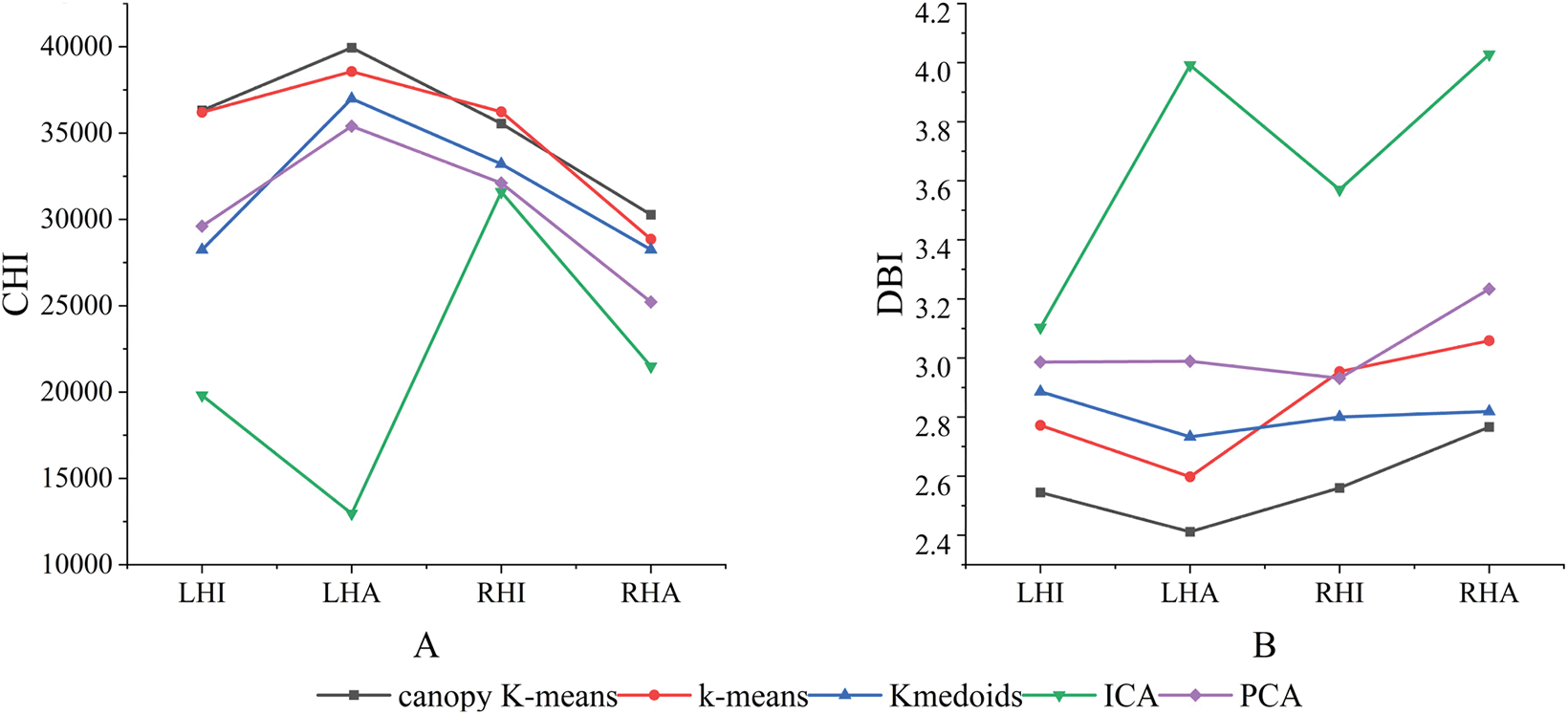
Figure 4: Clustering performance indicators of different algorithms (Note: A shows the CHI values of different clustering algorithms, and B shows the DBI values of different clustering algorithms. Abbreviations: LHI—Left hand imagined motion, LHA—Left hand actual motion, RHI—Right hand imagined motion, RHA—Right hand actual motion)

3.3 Microstate Characteristics

Microstate parameters, encompassing coverage, frequency of occurrence per second, and average duration, were extracted from the microstate sequences. Subsequent quantitative analyses were conducted to investigate the differences in microstate parameters between different tasks.

3.3.1 Coverage and Frequency of Occurrence per Second

Given the similarity of the coverage and frequency of occurrence per second data in the microstate parameters, we conduct a unified analysis. As illustrated in Fig. 5, the results indicate that microstates exhibit differences in different tasks. Particularly, microstate C demonstrates relatively high coverage and frequency of occurrence per second in the task, while microstate B and microstate E are relatively low. In microstate A, the coverage and frequency per second of imagined motion on both sides are relatively high. In microstate D, the coverage and frequency per second of actual motion on both sides are relatively high. Meanwhile, in the remaining three microstates, the coverage of different tasks is relatively consistent.

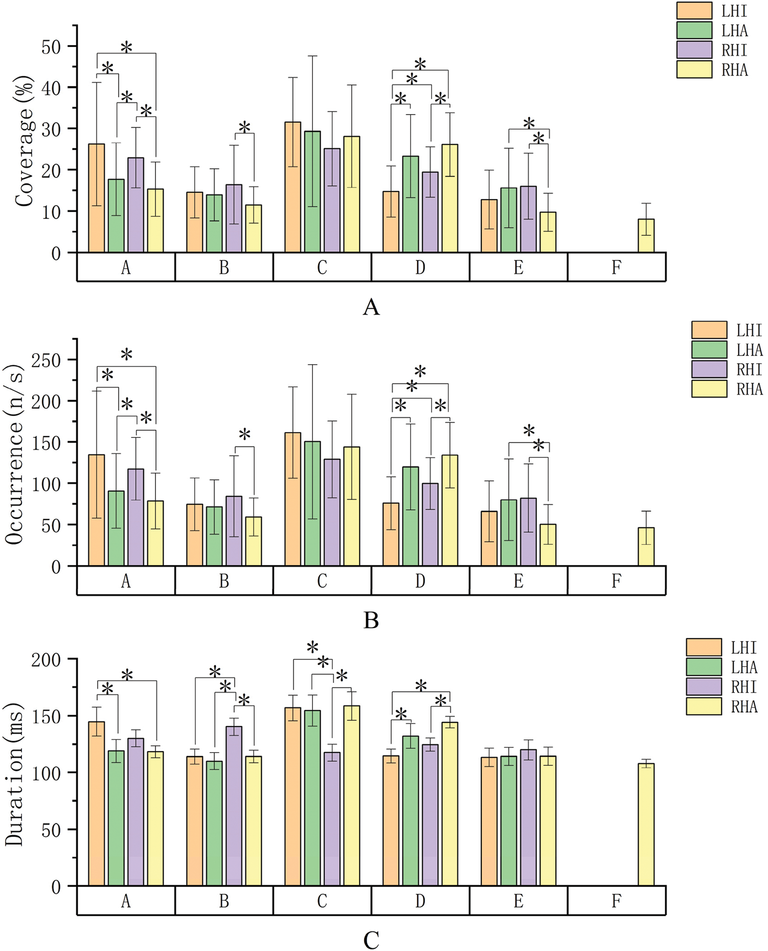
Figure 5: Microstate parameters (A shows the coverage range between different tasks, B shows the frequency of occurrence per second between different tasks, and C shows the average duration between different tasks. Abbreviations: LHI—Left hand imagined movement, LHA—Left hand actual movement, RHI—Right hand imagined movement, RHA—Right hand actual movement)

For microstate A, a significant difference was observed between left-hand imagined movements and both left-hand actual movements (p = 0.001) and right-hand actual movements (p = 0.000). Right-hand imagined movements were likewise significantly different from both left-hand actual movements (p = 0.046) and right-hand actual movements (p = 0.004). For microstate B, there was a significant difference between right-hand actual movements and right-hand imagined movements (p = 0.007). For microstate D, significant differences were observed between left-hand imagined movements and the remaining three tasks (p = 0.000, p = 0.022, p = 0.000), as well as between right-hand actual movements and right-hand imagined movements (p = 0.001). For microstate E, significant differences were observer between right-hand actual movements and left-hand actual movements, right-hand imagined movements (p = 0.004, p = 0.002).

3.3.2 Average Duration

Among the average durations of the different microstates, the average duration of microstate C was similarly higher. Within the same microstates, the duration of left-hand imagined movements was higher in microstate A; in microstate B, the duration of right-hand imagined movements was higher; and the duration of right-hand imagined movements was lower in microstate C. Microstates D and E exhibited more consistent durations across tasks.

For microstate A, there was a significant difference between left-hand imagined movement and lefthand actual movement and right-hand actual movement (p = 0.008, p = 0.007); for microstate B, there was a significant difference between right-hand imagined movement and all the remaining three types of tasks (p = 0.000, p = 0.000, p = 0.000); and for microstate C, again, there was a significant difference between right-hand imagined movement and the remaining three types of tasks (p = 0.001, p = 0.002, p = 0.001); for microstate D, there was a significant difference between left-hand imagined movement and left-hand actual Movement and right-hand actual movement (p = 0.023, p = 0.000), as well as a significant difference between right-hand imagined movement and right-hand actual movement (p = 0.011).

3.3.3 Probability of Microstate Transition

There were differences in the transition probabilities between different microstates, with a higher probability of transition from microstate E to microstate A in left-hand movements. Meanwhile, in the left-hand imagined motion, the transition probability of microstate E to microstate B is higher. In the left-hand actual motion, the transition probability of microstate D to microstate C is highest. In the right-hand imagined motion, the transition probability of microstate A and microstate E to microstate C is higher. In the right-hand actual motion, the transition probability of microstates C and D as well as E to microstate F is higher. The transfer probabilities between the various microstate topographies are shown in Table 1.

3.4 Characteristics of Microstate Sequences

In this study, four dynamic metrics, including Shannon entropy, entropy rate, sample entropy, and LZC, were used to measure the spatio-temporal complexity of various EEG dynamic state sequences comprehensively. As shown in Fig. 6, the parameters of actual motion, including Shannon entropy, sample entropy, entropy rate, and LZC complexity, are smaller than those of imagined motion on the same side.

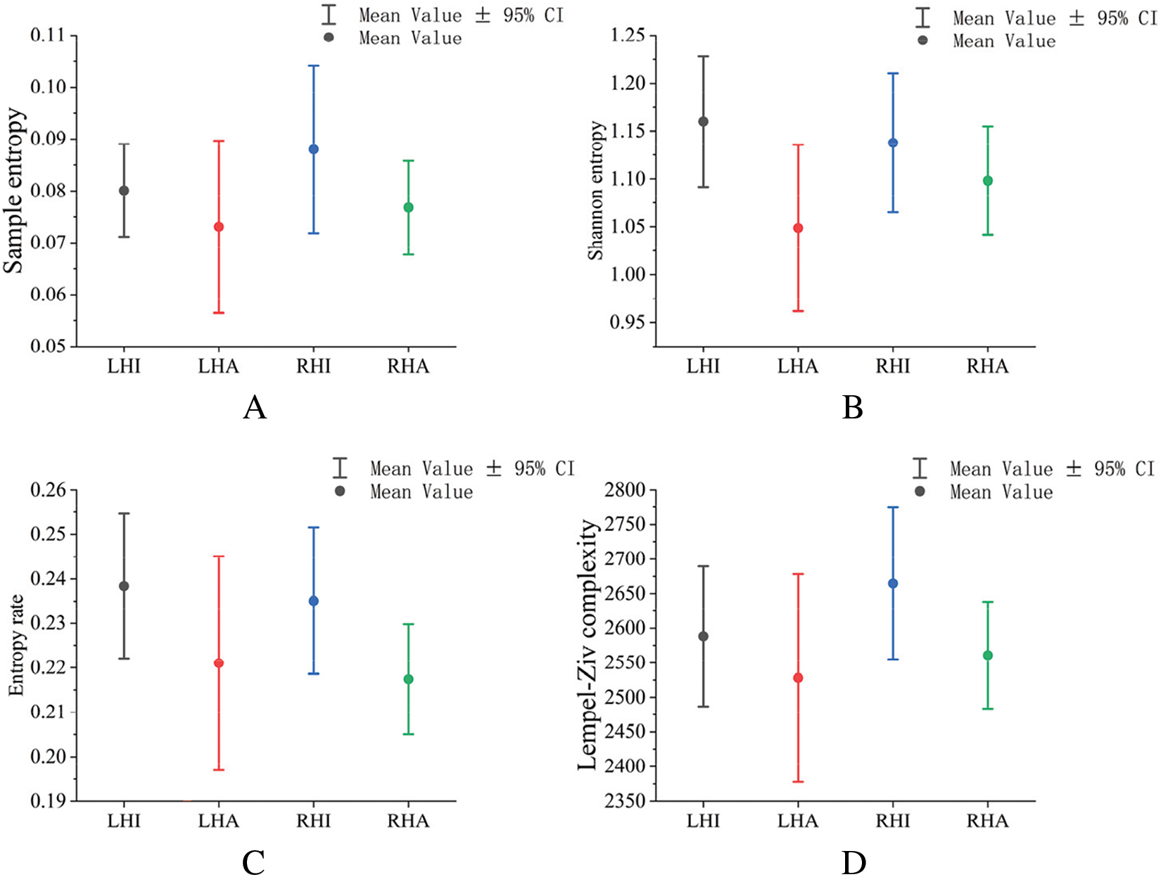
Figure 6: Dynamic feature parameters of microstate sequences clustered by an improved density canopy K-mean algorithm (note: A shows sample entropy for different tasks; B shows Shannon entropy for different tasks; C shows entropy rates for different tasks; D shows LZC complexity for different tasks. Abbreviations: LHI—Left hand imaginary movement, RHI—Right hand imaginary movement, LHA—Left hand actual movement, RHA—Right hand actual movement, Rest—Rest state)

3.5 Motion Imagination Recognition Based on Density Canopy K-Means

In order to validate the algorithm’s effectiveness, we applied the proposed clustering method to the recognition of different classes of motor imagery EEG signals, distinguishing between different tasks (left-hand actual motion and left-hand imagined motion, left-hand actual motion and right-hand actual motion, left-hand imagined motion and right-hand imagined motion, right-hand actual motion and right-hand imagined motion). For the binary classification problem, the formula for the accuracy is:

Accuracy=TP+TNTP+TN+FP+FN(15)

The feature set, derived from the improved clustering algorithm, was systematically divided into two distinct categories. Feature set 1 comprised microstate parameters, namely duration, frequency of occurrence, and coverage. Concurrently, feature set 2 integrated the fusion data of microstate parameters with microstate sequence features, including sample entropy, Shannon’s entropy, entropy rate, and LZC complexity. Subsequently, the resultant feature set was employed as input for a Support Vector Machine (SVM) classifier utilizing a Gaussian kernel.

As evident from Table 2, the GMD-driven density canopy K-means algorithm demonstrates notable performance in both feature sets. For feature set 1, the algorithm yields an average accuracy, specificity, and F1 score of 98.41%, 98.30%, and 98.38%, respectively. Similarly, for feature set 2, the algorithm achieves values of 98.41%, 98.81%, and 98.40% for average accuracy, specificity, and F1 score, respectively. Simultaneously, our method undergoes a comparative analysis with contemporary state-of-the-art approaches that have applied the same dataset.

In order to further validate the performance of the improved algorithm in motor imagery EEG signal classification, this paper applies the improved algorithm to the BCI Competition iv-2a dataset for the motor imagery four classification task. The dataset consists of a total of 5088 experiments for four motor imagery tasks, in which the experimental duration is 8 s and the MI task is completed in the middle 4 s. The performance of the improved algorithm in the motor imagery quad classification is shown in Table 3, where the accuracy of the quad classification for the motor imagery task reaches 78.105%, and its kappa score is 0.708. Its confusion matrix is shown in Fig. 7.

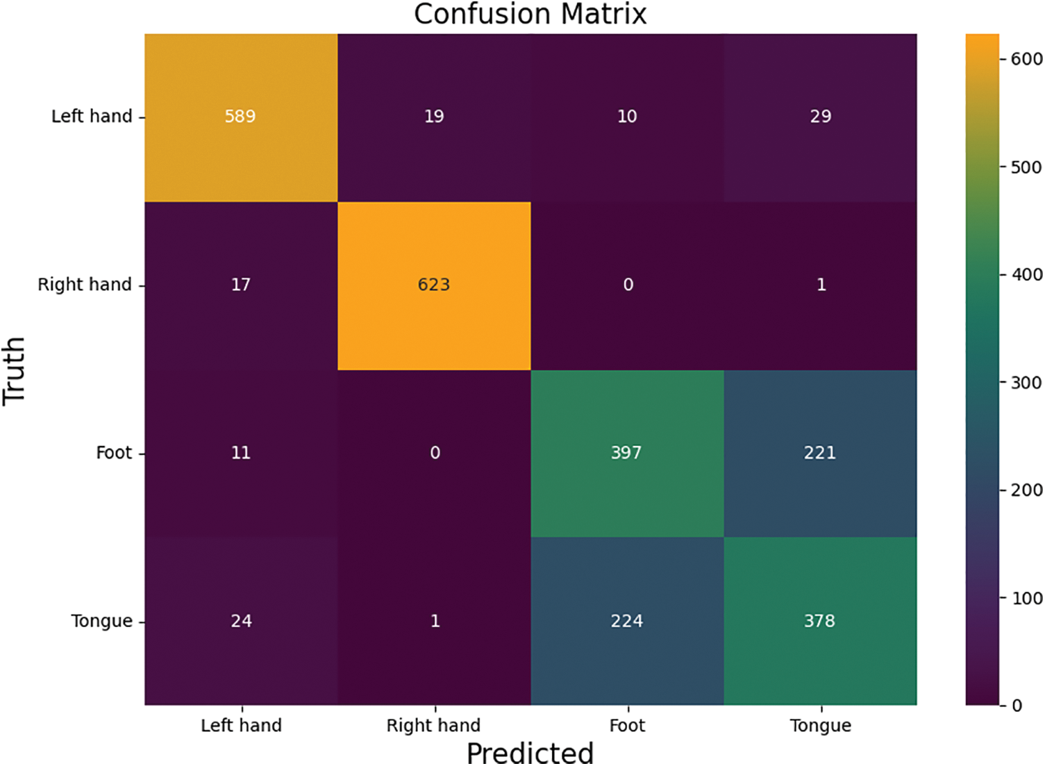
Figure 7: Confusion matrix of the BCI-iv-2a dataset

4  Discussion

In this study, the microstate topography maps were clustered by the GMD-driven density canopy K-means algorithm. Clustering of microstate topographies was performed for left-hand imagined motion, left-hand actual motion, and right-hand imagined motion, resulting in five clusters each. Additionally, six microstate topographies were clustered for right-hand actual motion [32].

However, whether the number of microstate topographies is driven by the EEG data itself has been a much debated issue [33]. In previous investigations, researchers have employed cross-validation guidelines to ascertain the optimal number of microstates [34], while others have posited that determining the optimal number should be a judicious amalgamation of experimental requirements and generalization considerations [32]. In the investigation of schizophrenia, the selection of four to six microstate topographies was contingent upon specific experimental conditions [35]. In a 2020 study on schizophrenia, six microstates were selected [17]. In 2021, Chen et al. introduced an AAHC algorithm based on dual thresholding for the recognition of EEG signals. The study yielded 9 and 10 microstates across different emotion analysis datasets [36]. In 2022, an analysis of brain work tasks involving distinct information types resulted in the identification of six microstates [37]. In our study, we present a GMD-driven density canopy K-means algorithm which determines the most compact clustering centers through an analysis of the dataset’s density and GMD index. This approach provides a more objective consideration of the distribution of dataset samples, addressing the challenge of determining T1 and T2 parameters inherent in the traditional Canopy algorithm.

Following the application of the algorithm to model motor imagery EEG signals in this study, a comparative analysis was conducted between the microstate topographies obtained herein and those of traditional microstate maps. Remarkably, all derived microstate topographies exhibited a high degree of similarity with the original microstate topographies. The microstates A and B identified in this study corresponded directly to the traditional microstates A and B. In microstate A, the coverage, frequency of occurrence, and average duration associated with imagined motion on both sides surpass those of the actual motion. This suggests that during motor imagery, subjects relied predominantly on neural activities associated with sensory modalities such as vision and hearing [38], leading to an enhanced salience of microstate A in these tasks. This suggests that the nature of motor imagery tasks may be linked to the activity of brain regions associated with perception and cognition [39]. Simultaneously, both microstate C and microstate D in this study exhibited similarities with the traditional microstate C. Furthermore, in this study, microstate C demonstrated higher values for coverage, frequency of occurrence, and average duration compared to the other microstates. Significant differences were observed between right-hand imagery movement and the remaining tasks. Simultaneously, our study revealed an association of microstate C with neuronal activity in the prefrontal and anterior temporal lobes, recognized as core regions for cognitive and behavioral functions. Li et al. demonstrated that the parietal motor cortex may be more influenced by the cognitive prefrontal cortex [40]. In the microstate D of the present study, notable differences were observed among various types of tasks. These differences corresponded to the central gyrus, precentral gyrus, and frontal region, indicative of the main motor cortex. The presence of significant differences among various types of tasks suggests that motor imagery and actual movement engage distinct neural mechanisms. Actual movement engages executive functions in the central gyrus and precentral gyrus, whereas motor imagery may encompass additional cognitive and attentional control, potentially leading to more pronounced activity in frontal regions [41]. Microstate E and microstate F in the present study correspond to the traditional microstate D, linked with the dorsal attentional network and indicative of heightened attention and shifts in focus. The inclusion of microstate F during right-hand actual movement, compared to the other tasks, more accurately captures the increased attention demanded by actual movement. This heightened attention is attributed to the involvement of physical body movement, muscle control, and sensory feedback, necessitating additional cognitive resources for coordination and execution.

We further analyzed the motor imagery data using the dynamic eigenvalues extracted by the improved algorithm, demonstrating their significant superiority over the traditional algorithm in various aspects. More specifically, the eigenvalues extracted by the improved algorithm demonstrated a broader range of values in the spatio-temporal complexity description and exhibited heightened variability. This further underscores the reliability and superior performance of the improved algorithm. Remarkably, we observed that various parameters associated with actual movement, namely Shannon entropy, sample entropy, entropy rate, and LZC complexity [31], all exhibit smaller values compared to the parameters of ipsilateral imagined motion. This finding suggests that brain activity during actual movement is characterized by greater orderliness and consistency. This observation may imply that actual movements engage relatively more well-defined neural activities, primarily concentrated in the sensorimotor regions of the brain. In contrast, imagined movements may necessitate increased neural activity to simulate sensations and actions of movement in the brain, resulting in higher complexity [42,43].

In order to further verify the superiority of the improved clustering algorithm, this experiment is compared with the classical microstate clustering algorithm, and the clustering performance of the different algorithms is specifically measured by the three parameters, namely, the GEV value, the CHI index, and the DBI index. Specifically, the increase in the GEV value implies that the improved algorithm more effectively preserves the overall variability of the original data, showing its more superior clustering effect on a global scale. The GEV value of the improved algorithm (GEV = 0.746) is higher than that of the K-means algorithm, the kmedoids algorithm, the ICA algorithm, and the PCA algorithm. The excellent performance of the improved algorithm in microstate analysis can be partly attributed to its superiority in noise filtering in EEG data. Compared to the traditional K-means algorithm, the improved algorithm filters out the effects from noise sources such as eye-point artifacts, muscle artifacts, and so on more efficiently through a density-crown-based strategy. This feature makes the improved algorithm more robust and able to capture the real features in the EEG data more accurately, which improves the accuracy and reliability of microstate analysis. Meanwhile, the CHI index of the improved algorithm (CHI = 35517.29) is better than the rest of the algorithms, which demonstrates that the improved algorithm can better capture the differences between different task states and has higher sensitivity in recognizing the main task states. Contrary to the CHI index, we find that the DBI index (DBI = 2.57) of the improved algorithm is generally smaller than the rest of the algorithms. This indicates that the improved algorithm has a clearer separation between different task states and a greater variability between different task states.

To further demonstrate the inherent superiority of the improved algorithm, this experiment compares the GMD-driven density canopy K-means algorithm with the Teager energy operator-based microstate analysis method. Experiments were conducted to correlate the left-handed imagined motion with the right-handed imagined motion in the BCI-iv-2a dataset for microstate analysis. Significant differences in the microstate parameter analysis between the different methods were found, starting with six microstates in left-handed imagined motion and five microstates in right-handed imagined motion using the algorithm in this paper. In addition, in terms of the analysis of microstate parameters, the different microstate parameters obtained by this paper’s algorithm were significantly different between the left and right hand imagined motions (tCOV¯ = 82.126, pCOV¯ = 0.00; tOCC¯ = 78.174, pOCC¯ = 0.00; and tDUR¯ = 31.907, pDUR¯ = 0.00). The results were superior to those of the microstate analysis method based on Teager’s energy operator. This proves that the improved algorithm can better distinguish the differences between different task states in terms of microstate analysis.

In order to verify the effectiveness of the present algorithm more rigorously, we performed classification tests for the motor imagery task. In the present dataset, the average classification accuracy using the present algorithm is as high as 98.41%, and in the BCI-iv-2a dataset, the classification accuracy for left- and right-handed imagined motions is even more impressive at 99.84%. Comparing this result with microstate studies using the same database, it is not difficult to find the advantages of the present algorithm. Specifically, Liu et al. used microstate analysis for the classification of left- and right-handed imaginative motions with an accuracy of 89.17% [44], whereas Li et al.’s microstate analysis method based on the Teager energy operator obtained a classification accuracy of 93.93% [45]. Obviously, the present algorithm shows higher efficacy in microstate analysis. However, we also note that the accuracy of the present algorithm drops to 78.1% when coping with the four-classification task on the BCI-iv-2a dataset, with a Kappa score of 0.708. In contrast, the Dynamic Attentional Temporal Convolutional Network (D-ATCNet) proposed by Hamdi et al. [46] performs well in the four-classification task, especially in the subject-dependent case, and the classification accuracy reached 87.08%. This suggests that the performance of the present algorithm could be improved in more complex classification tasks. Nevertheless, the microstate analysis method still has its unique advantages. Compared with convolutional neural networks, microstate analysis shows good interpretability in the analysis process, and can reveal the spatio-temporal dynamic differences between different motion imagery tasks in more depth. Therefore, in future research, we will aim to further optimize the present algorithm with a view to improving its performance in complex classification tasks while maintaining high interpretability.

We plan to introduce more advanced clustering algorithms in our future research work to enhance its ability to cope with complex work scenarios. Specifically, the deep spectral clustering algorithm, with its powerful feature learning and clustering capabilities, will be our focus. In addition, the successful application of convolutional neural networks in the field of image recognition provides us with insights that we can try to apply them to microstate analysis to capture deeper feature information. In addition to algorithmic level improvements, we will also work on extracting more accurate and effective feature parameters in microstate analysis to further improve the classification results. This will help us recognize different categories of motion imagery more accurately and provide a more reliable basis for practical applications.

5  Conclusion

Founded on the conventional K-means algorithm, in this paper the GMD-driven density canopy K-means algorithm is introduced. The proposed clustering method has been successfully employed in the classification and recognition of motor imagery EEG signals, yielding commendable outcomes in terms of recognition and detection. The research findings emphasize the significant enhancement in the recognition performance of motor imagery EEG signals achieved by this algorithm.

In summary, the GMD-driven density canopy K-means algorithm represents an important step forward in the field of EEG signal analysis and motor image recognition. By overcoming the inherent limitations of traditional microstate analysis methods, the algorithm provides a more in-depth and detailed analysis framework for EEG signals, thus revealing many key details that have been neglected in the past. This not only has a positive impact on the improvement of motion image recognition technology, but also provides a brand new idea and direction for the further improvement and innovation of microstate analysis methods. The emergence of this algorithm not only promotes the theoretical development of related disciplines, but also lays a solid foundation for its extensive promotion in practical applications.

In our future research program, we envision a series of research directions with depth. First, we aim to further broaden the application of the algorithm, especially for neural signal analysis in the context of different cognitive tasks. Second, we plan to deeply integrate the microstate clustering approach with a series of cutting-edge machine learning techniques, e.g., deep spectral clustering and convolutional neural networks. We expect to significantly improve the overall performance of EEG signal analysis. Finally, we would like to conduct more comprehensive experiments to verify the generalization and robustness of our algorithms in different datasets and experimental environments.

Acknowledgement: The authors would like to thank the laboratory for providing the computing resources for the development of this study.

Funding Statement: This research was funded by National Nature Science Foundation of China, Yunnan Funda-Mental Research Projects, Special Project of Guangdong Province in Key Fields of Ordinary Colleges and Universities and Chaozhou Science and Technology Plan Project of Funder Grant Numbers 82060329, 202201AT070108, 2023ZDZX2038 and 202201GY01.

Author Contributions: The authors confirm contribution to the paper as follows: Conceptualization, X.X.; methodology, J.Z.; software, J.Z.; validation, X.X. and R.L.; formal analysis, X.X.; investigation, S.Y.; resources, X.X.; data curation, C.W.; draft manuscript preparation, X.X. and J.Z.; visualization, J.Z.; supervision, J.H.; project administration, X.X.; funding acquisition, J.H. All authors reviewed the results and approved the final version of the manuscript.

Availability of Data and Materials: The experimental data for this study were sourced from the GigaScience database (http://dx.doi.org/10.5524/100295).

Conflicts of Interest: The author declare that they have no conflicts of interest to report regarding the present study.

References

1. S. Eldeeb et al., “EEG-based functional connectivity to analyze motor recovery after stroke: A pilot study,” Biomed. Signal Process. Control, vol. 49, pp. 419–426, 2019. doi: 10.1016/j.bspc.2018.12.022. [Google Scholar] [CrossRef]

2. J. G. Bogaarts, E. D. Gommer, D. M. W. Hilkman, V. H. J. M. van Kranen-Mastenbroek, and J. P. H. Reulen, “EEG feature pre-processing for neonatal epileptic seizure detection,” Ann. Biomed. Eng., vol. 42, no. 11, pp. 2360–2368, 2014. doi: 10.1007/s10439-014-1089-2. [Google Scholar] [PubMed] [CrossRef]

3. E. Barzegaran, B. van Damme, R. Meuli, and M. G. Knyazeva, “Perception-related EEG is more sensitive to Alzheimer’s disease effects than resting EEG,” Neurobiol. Aging, vol. 43, pp. 129–139, 2016. doi: 10.1016/j.neurobiolaging.2016.03.032. [Google Scholar] [PubMed] [CrossRef]

4. A. J. Doud, J. P. Lucas, M. T. Pisansky, and B. He, “Continuous three-dimensional control of a virtual helicopter using a motor imagery based brain-computer interface,” PLoS One, vol. 6, no. 10, pp. e26322, 2011. doi: 10.1371/journal.pone.0026322. [Google Scholar] [PubMed] [CrossRef]

5. T. Carlson and J. D. R. Millan, “Brain-controlled wheelchairs: A robotic architecture,” IEEE Robot. Automat. Mag., vol. 20, no. 1, pp. 65–73, 2013. doi: 10.1109/MRA.2012.2229936. [Google Scholar] [CrossRef]

6. W. C. Hsu, L. F. Lin, C. W. Chou, Y. T. Hsiao, and Y. H. Liu, “EEG classification of imaginary lower limb stepping movements based on fuzzy support vector machine with kernel-induced membership function,” Int. J. Fuzzy Syst., vol. 19, no. 2, pp. 566–579, 2017. doi: 10.1007/s40815-016-0259-9. [Google Scholar] [CrossRef]

7. O. W. Samuel, Y. Geng, X. Li, and G. Li, “Towards efficient decoding of multiple classes of motor imagery limb movements based on EEG spectral and time domain descriptors,” J. Med. Syst., vol. 41, no. 12, pp. 1–13, 2017. doi: 10.1007/s10916-017-0843-z. [Google Scholar] [PubMed] [CrossRef]

8. M. Tavakolan, X. Yong, X. Zhang, and C. Menon, “Classification scheme for arm motor imagery,” J. Med. Biol. Eng., vol. 36, no. 1, pp. 12–21, 2016. doi: 10.1007/s40846-016-0102-7. [Google Scholar] [PubMed] [CrossRef]

9. K. K. Ang, Z. Y. Chin, H. Zhang, and C. Guan, “Filter bank common spatial pattern (FBCSP) in brain-computer interface,” presented at the 2018 IEEE World Conf. Comput. Intell., Hong Kong, China, Nov. 6–1, 2008. doi: 10.1109/IJCNN.2008.4634130. [Google Scholar] [CrossRef]

10. J. Dinarès-Ferran, R. Ortner, C. Guger, and J. Solé-Casals, “A new method to generate artificial frames using the empirical mode decomposition for an EEG-based motor imagery BCI,” Front. Neurosci., vol. 12, pp. 360144, 2018. doi: 10.3389/fnins.2018.00308. [Google Scholar] [PubMed] [CrossRef]

11. B. J. Edelman, B. Baxter, and B. He, “EEG source imaging enhances the decoding of complex right-hand motor imagery tasks,” IEEE Trans. Biomed. Eng., vol. 63, no. 1, pp. 4–14, 2015. doi: 10.1109/TBME.2015.2467312. [Google Scholar] [PubMed] [CrossRef]

12. Y. Chu et al., “Decoding multiclass motor imagery EEG from the same upper limb by combining Riemannian geometry features and partial least squares regression,” J. Neural Eng., vol. 17, no. 4, pp. 046029, 2020. doi: 10.1088/1741-2552/aba7cd. [Google Scholar] [PubMed] [CrossRef]

13. H. Altaheri et al., “Deep learning techniques for classification of electroencephalogram (EEG) motor imagery (MI) signals: A review,” Neural Comput. Appl., vol. 35, no. 20, pp. 14681–14722, 2023. doi: 10.1007/s00521-021-06352-5. [Google Scholar] [CrossRef]

14. D. Lehmann, Brain Electric Microstates and Cognition: The Atoms of Thought. Boston: Birkhäuser, 1990. doi: 10.1007/978-1-4757-1083-0_10. [Google Scholar] [CrossRef]

15. G. S. Wu et al., “Microstate dynamics and spectral components as markers of persistent and remittent attention-deficit/hyperactivity disorder,” Clin. Neurophysiol., vol. 161, no. 7, pp. 147–156, 2024. doi: 10.1016/j.clinph.2024.02.027. [Google Scholar] [PubMed] [CrossRef]

16. C. Chu et al., “Temporal and spatial variability of dynamic microstate brain network in early Parkinson’s disease,” npj Parkinson's Dis., vol. 9, no. 1, pp. 57, 2023. doi: 10.1038/s41531-023-00498-w. [Google Scholar] [PubMed] [CrossRef]

17. Y. Luo, Q. Tian, C. Wang, K. Zhang, C. Wang and J. Zhang, “Biomarkers for prediction of schizophrenia: Insights from resting-state EEG microstates,” IEEE Access, vol. 8, pp. 213078–213093, 2020. doi: 10.1109/ACCESS.2020.3037658. [Google Scholar] [CrossRef]

18. F. von Wegner, P. Knaut, and H. Laufs, “EEG microstate sequences from different clustering algorithms are information-theoretically invariant,” Front. Comput. Neurosci., vol. 12, pp. 70, 2018. doi: 10.3389/fncom.2018.00070. [Google Scholar] [PubMed] [CrossRef]

19. K. M. Spencer, J. Dien, and E. Donchin, “A componential analysis of the ERP elicited by novel events using a dense electrode array,” Psychophysiology, vol. 36, no. 3, pp. 409–414, 1999. doi: 10.1017/S0048577299981180. [Google Scholar] [PubMed] [CrossRef]

20. L. Tait et al., “EEG microstate complexity for aiding early diagnosis of Alzheimer’s disease,” Sci. Rep., vol. 10, no. 1, pp. 17627, 2020. doi: 10.1038/s41598-020-74790-7. [Google Scholar] [PubMed] [CrossRef]

21. H. Jia and D. Yu, “Aberrant intrinsic brain activity in patients with autism spectrum disorder: Insights from EEG microstates,” Brain Topogr., vol. 32, no. 2, pp. 295–303, 2019. doi: 10.1007/s10548-018-0685-0. [Google Scholar] [PubMed] [CrossRef]

22. T. Kleinert, T. Koenig, K. Nash, and E. Wascher, “On the reliability of the EEG microstate approach,” Brain Topogr., vol. 37, no. 2, pp. 271–286, 2024. doi: 10.1007/s10548-023-00982-9. [Google Scholar] [PubMed] [CrossRef]

23. K. Kim, N. T. Duc, M. Choi, and B. Lee, “EEG microstate features for schizophrenia classification,” PLoS One, vol. 16, no. 5, pp. e0251842, 2021. doi: 10.1371/journal.pone.0251842. [Google Scholar] [PubMed] [CrossRef]

24. T. Huang, S. Liu, and Y. Tan, “Research of clustering algorithm based on K-means,” Comp. Technol. Dev., vol. 21, no. 7, pp. 54–57, 2011. [Google Scholar]

25. J. Wang, S. T. Wang, and Z. H. Deng, “A novel text clustering algorithm based on feature weighting distance and soft subspace learning,” (in ChineseJisuanji Xuebao (Chinese J. Comput.), vol. 35, no. 8, pp. 1655–1665, 2012. doi: 10.3724/SP.J.1016.2012.01655. [Google Scholar] [CrossRef]

26. J. Xie, S. Jiang, W. Xie, and X. Gao, “An efficient global K-means clustering algorithm,” J. Comput., vol. 6, no. 2, pp. 271–279, 2011. doi: 10.4304/jcp.6.2.271-279. [Google Scholar] [CrossRef]

27. S. B. Zhou, Z. Y. Xu, and X. Q. Tang, “Method for determining optimal number of clusters in K-means clustering algorithm,” J. Comput. Appl., vol. 30, no. 8, pp. 1995–1998, 2010. doi: 10.3724/SP.J.1087.2010.01995. [Google Scholar] [CrossRef]

28. D. Mao, “Improved canopy-ameans algorithm based on MapReduce,” Jisuanji Gongcheng yu Yingyong (Comput. Eng. Appl.), vol. 48, pp. 27, 2012. doi: 10.1109/cisp-bmei.2016.7853042. [Google Scholar] [CrossRef]

29. G. Zhang, C. Zhang, and H. Zhang, “Improved K-means algorithm based on density canopy,” Knowl. Based Syst., vol. 145, no. 6, pp. 289–297, 2018. doi: 10.1016/j.knosys.2018.01.031. [Google Scholar] [CrossRef]

30. Y. Mohammadi and M. H. Moradi, “Prediction of depression severity scores based on functional connectivity and complexity of the EEG signal,” Clin. EEG Neurosci., vol. 52, no. 1, pp. 52–60, 2021. doi: 10.1177/1550059420965431. [Google Scholar] [PubMed] [CrossRef]

31. X. Liu et al., “Multiple characteristics analysis of Alzheimer’s electroencephalogram by power spectral density and Lempel-Ziv complexity,” Cogn. Neurodyn., vol. 10, no. 2, pp. 121–133, 2016. doi: 10.1007/s11571-015-9367-8. [Google Scholar] [PubMed] [CrossRef]

32. C. M. Michel and T. Koenig, “EEG microstates as a tool for studying the temporal dynamics of whole-brain neuronal networks: A review,” Neuroimage, vol. 180, no. Suppl. 1, pp. 577–593, 2018. doi: 10.1016/j.neuroimage.2017.11.062. [Google Scholar] [PubMed] [CrossRef]

33. J. Liu, J. Xu, G. Zou, Y. He, Q. Zou and J. H. Gao, “Reliability and individual specificity of EEG microstate characteristics,” Brain Topogr., vol. 33, no. 4, pp. 438–449, 2020. doi: 10.1007/s10548-020-00777-2. [Google Scholar] [PubMed] [CrossRef]

34. S. P. Muthukrishnan, N. Ahuja, N. Mehta, and R. Sharma, “Functional brain microstate predicts the outcome in a visuospatial working memory task,” Behav. Brain Res., vol. 314, pp. 134–142, 2016. doi: 10.1016/j.bbr.2016.08.020. [Google Scholar] [PubMed] [CrossRef]

35. S. Soni, S. P. Muthukrishnan, M. Sood, S. Kaur, and R. Sharma, “Hyperactivation of left inferior parietal lobule and left temporal gyri shortens resting EEG microstate in schizophrenia,” Schizophr. Res., vol. 201, no. Suppl 1, pp. 204–207, 2018. doi: 10.1016/j.schres.2018.06.020. [Google Scholar] [PubMed] [CrossRef]

36. J. Chen, H. Li, L. Ma, H. Bo, F. Soong, and Y. Shi, “Dual-threshold-based microstate analysis on characterizing temporal dynamics of affective process and emotion recognition from EEG signals,” Front. Neurosci., vol. 15, pp. 689791, 2021. doi: 10.3389/fnins.2021.689791. [Google Scholar] [PubMed] [CrossRef]

37. K. Guan, Z. Zhang, X. Chai, Z. Tian, T. Liu and H. Niu, “EEG based dynamic functional connectivity analysis in mental workload tasks with different types of information,” IEEE Trans. Neural Syst. Rehabil. Eng., vol. 30, pp. 632–642, 2022. doi: 10.1109/tnsre.2022.3156546. [Google Scholar] [PubMed] [CrossRef]

38. D. F. D’Croz-Baron, L. Bréchet, M. Baker, and T. Karp, “Auditory and visual tasks influence the temporal dynamics of EEG microstates during post-encoding rest,” Brain Topogr., vol. 34, no. 1, pp. 19–28, 2021. doi: 10.1007/s10548-020-00802-4. [Google Scholar] [PubMed] [CrossRef]

39. H. O’Shea, “Mapping relational links between motor imagery, action observation, action-related language, and action execution,” Front. Hum. Neurosci., vol. 16, pp. 984053, 2022. doi: 10.3389/fnhum.2022.984053. [Google Scholar] [PubMed] [CrossRef]

40. L. Li et al., “Activation of the brain during motor imagination task with auditory stimulation,” Front. Neurosci., vol. 17, pp. 1130685, 2023. doi: 10.21203/rs.3.rs-1136249/v1. [Google Scholar] [CrossRef]

41. T. Hanakawa, I. Immisch, K. Toma, M. A. Dimyan, P. van Gelderen and M. Hallett, “Functional properties of brain areas associated with motor execution and imagery,” J. Neurophysiol., vol. 89, no. 2, pp. 989–1002, 2003. doi: 10.1152/jn.00132.2002. [Google Scholar] [PubMed] [CrossRef]

42. N. Sharma et al., “Motor imagery after subcortical stroke: A functional magnetic resonance imaging study,” Stroke, vol. 40, no. 4, pp. 1315–1324, 2009. doi: 10.1161/strokeaha.108.525766. [Google Scholar] [PubMed] [CrossRef]

43. A. Guillot, C. Collet, V. A. Nguyen, F. Malouin, C. Richards and J. Doyon, “Brain activity during visual versus kinesthetic imagery: An fMRI study,” Hum. Brain Mapp., vol. 30, no. 7, pp. 2157–2172, 2009. doi: 10.1002/hbm.20658. [Google Scholar] [PubMed] [CrossRef]

44. W. Liu, X. Liu, R. Dai, and X. Tang, “Exploring differences between left and right hand motor imagery via spatio-temporal EEG microstate,” Comput. Assist. Surg., vol. 22, no. supl, pp. 258–266, 2017. doi: 10.1080/24699322.2017.1389404. [Google Scholar] [PubMed] [CrossRef]

45. Y. Li, M. Chen, S. Sun, and Z. Huang, “Exploring differences for motor imagery using Teager energy operator-based EEG microstate analyses,” J. Integr. Neurosci., vol. 20, no. 2, pp. 411–417, 2021. doi: 10.31083/j.jin2002042. [Google Scholar] [PubMed] [CrossRef]

46. H. Altaheri, G. Muhammad, and M. Alsulaiman, “Dynamic convolution with multilevel attention for EEG-based motor imagery decoding,” IEEE Internet Things J., vol. 10, no. 21, pp. 18579–18588, 2023. doi: 10.1109/JIOT.2023.3281911. [Google Scholar] [CrossRef]