Coupling Analysis of Multiple Machine Learning Models for Human Activity Recognition

1  Introduction

Human activity recognition (HAR) is a key technology for the surveillance of rehabilitation and fitness for healthcare applications in smart cities [1,2]. Many emerging HAR methods have been developed in the areas of signal, image, and video analysis technology due to surveillance in various dimensions. The technology enabled the automatic recognition of patient’s daily activities, abnormal gestures, and rehabilitation processes with artificial intelligence (AI) in healthcare applications [3]. Non-image signal analysis is particularly helpful in a healthcare system for privacy concerns. Various machine learning (ML) models are proposed to improve recognition accuracy significantly, boosting comprehension of human postures and movements for AI computing. An HAR framework usually contains four steps, i.e., collecting, preprocessing, featuring, and labeling data segments, to prepare samples before data training [4].

The base of ML algorithms was assorted with two types: non-iteration and iteration. The non-iteration-based algorithm classifies multiclass labels of the features based on classification formulations. The support vector machine (SVM) and random forest (RF) with ensemble analysis were popular in identifying the HAR data in the past decades [5–7]. The iteration-based algorithm drives the forward and backward iterations in the multiple-layer neural networks (NN) for modeling the optimal structure. The adaptive neural fuzzy inference system (ANFIS), which combines an artificial neural network (ANN) and a fuzzy inference system (FIS), is a typical method [8,9]. In the last decade, the convolutional neural network (CNN) initiatively filtered delicate features for deeply learning data segments and became an import subset of ML methods [10,11]. The ANFIS, SVM, RF, and CNN algorithms, which were sequentially invented in the past four decades, could be integrated with AI computing and data identification for the HAR applications.

Many open databases help train various ML models to improve the modern HAR technique. The UCI-HAR was a well-known open database measuring thirty subjects for HAR modeling [12]. With default design, measurement data of twenty-one and nine subjects were arranged for training and testing, respectively. Each subject wore a smartphone on the waist and executed six activities. The datasets also include 561 feature variables in time and frequency domains to download for learning. The MHEALTH was also a popular open database that offers the measurement of twelve activities by locating the sensors, including accelerometers, gyroscopes, and magnetometers, on the subject’s chest, left ankle, and right arm in high-performance modeling for complex-classes HAR [13]. The study recruited ten subjects wearing three sensors on the chest, left ankle, and right-lower arm to collect signals of acceleration, angular velocity, and magnetic field along three axes. In addition, the WISDM database measured eighteen lifestyle activities of fifty-one subjects with the accelerometers and gyroscopes of smartwatches and smartphones, which was challenging for HAR applications [14]. The raw data could be converted to diverse features for machine learning.

In general, the ML methods require preparing features for data training. An efficient featuring process can improve the efficacy of the ML models. The conventional ML methods requested massive features to enhance the model’s recognition capability, but redundant features increased the overall computational complexity [15,16]. A recursive feature elimination (RFE) method was suggested to explore the most relevant features for recognition [17]. Recently, the deep learning (DL) technique has been known to automatically discover features with high performance in HAR. In recent years, numerous DL methods have been explored to accomplish various HAR approaches [18]. The advanced DL methods, such as CNN, could initiatively filter possible features via convolutional operation in the network layers, but degradation occurred in the deep layers. The squeeze-and-excitation (SE) block and residual blocks derived from the CNN were advised to avoid degradation [19,20]. The hybrid CNNs became a strategy to improve the model’s effectiveness.

In this study, we contributed a coupling analysis framework to design proposed HAR models with an efficient machine learning process using three open databases. We first applied the UCI-HAR to build multiple ML and DL models based on ANFIS, SVM, RF, and hybrid CNNs for coupling analysis. The MHEALTH was further employed to repeat the modeling process for comparison. Finally, the WISDM was applied to application to approve the framework’s robustness and versatility. In this article, the framework was designed in the methods section, followed by the results and discussions sections, and then a conclusion was addressed in the last section.

2  Methods

This study engaged the UCI-HAR to train the proposed models and applied the MHEALTH for comparative modeling. Besides the raw measured signals, at most, 561 feature variables in time and frequency domains can also be downloaded on the UCI-HAR website for machine learning. The functions used to derive UCI-HAR’s features were referred to convert MHEALTH’s raw signals to the possible features. In this study, the “fitcecoc” and “anfis” functions, built-in MATLABTM (license no. 40660563) toolbox, were employed to drive the SVM, RF, and ANFIS methods, respectively, for ML-based models. Python’s “tensorflow” library was also applied to establish a DL-based model using the hybrid CNNs method.

2.1 UCI-HAR Open Dataset

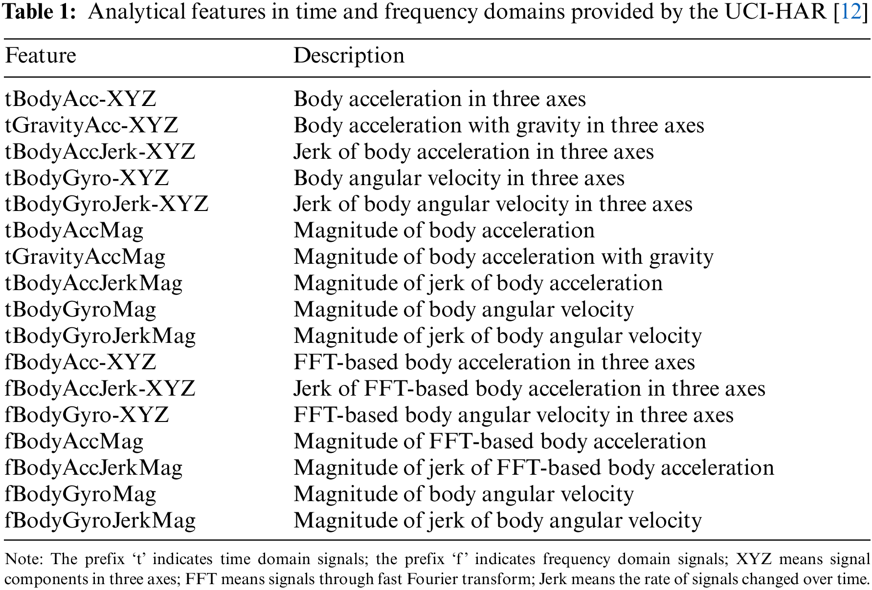
The UCI-HAR project recruited thirty subjects wearing smartphones on their waists to exercise six activities. According to the downloaded data, 21 subjects were arranged for training in ML, while the other 9 subjects were for testing (i.e., train-test ratio is 7:3). We denoted the segments of walking, walking upstairs, walking downstairs, sitting, standing, and laying activities by labels: {walk, wu, wd, sit, sta, lay}, in which the number of training and testing datasets were {1226, 1073, 986, 1286, 1374, 1407} and {496, 471, 420, 491, 532, 537}, respectively. Due to the experiment, an accelerometer and a gyroscope embedded in the smartphone could collect signals of acceleration, acceleration with gravity, and angular velocity. Each physical quantity contains x, y, and z axial components parallel to the human body’s up-down, left-right, and front-rear directions. The raw signals were measured at a frequency of 50 Hz. All data segments were processed by a Butterworth low-pass filter with a cutoff frequency 0.3 Hz to remove noises. Each segment sampled by a sliding window of 128 timestamps with 50% overlap was converted to analytical features in time and frequency domains, as shown in Table 1. The features were transformed into 561 potential features, as referred to in Table S1, for machine learning, while the sample segments of raw signals tBodyAcc-XYZ, tGravityAcc-XYZ, and tBodyGyro-XYZ were applied for DL.

2.2 Classic Learning Algorithms

For comparison, we generated analytical models based on four conventional ML and DL algorithms that were the most representative methods for each decade in the past 40 years. The algorithms for the proposed models are briefly addressed below for the article’s integrity. Their parameters are shown in Table 2, and the DL model’s architecture is illustrated in Fig. 1.

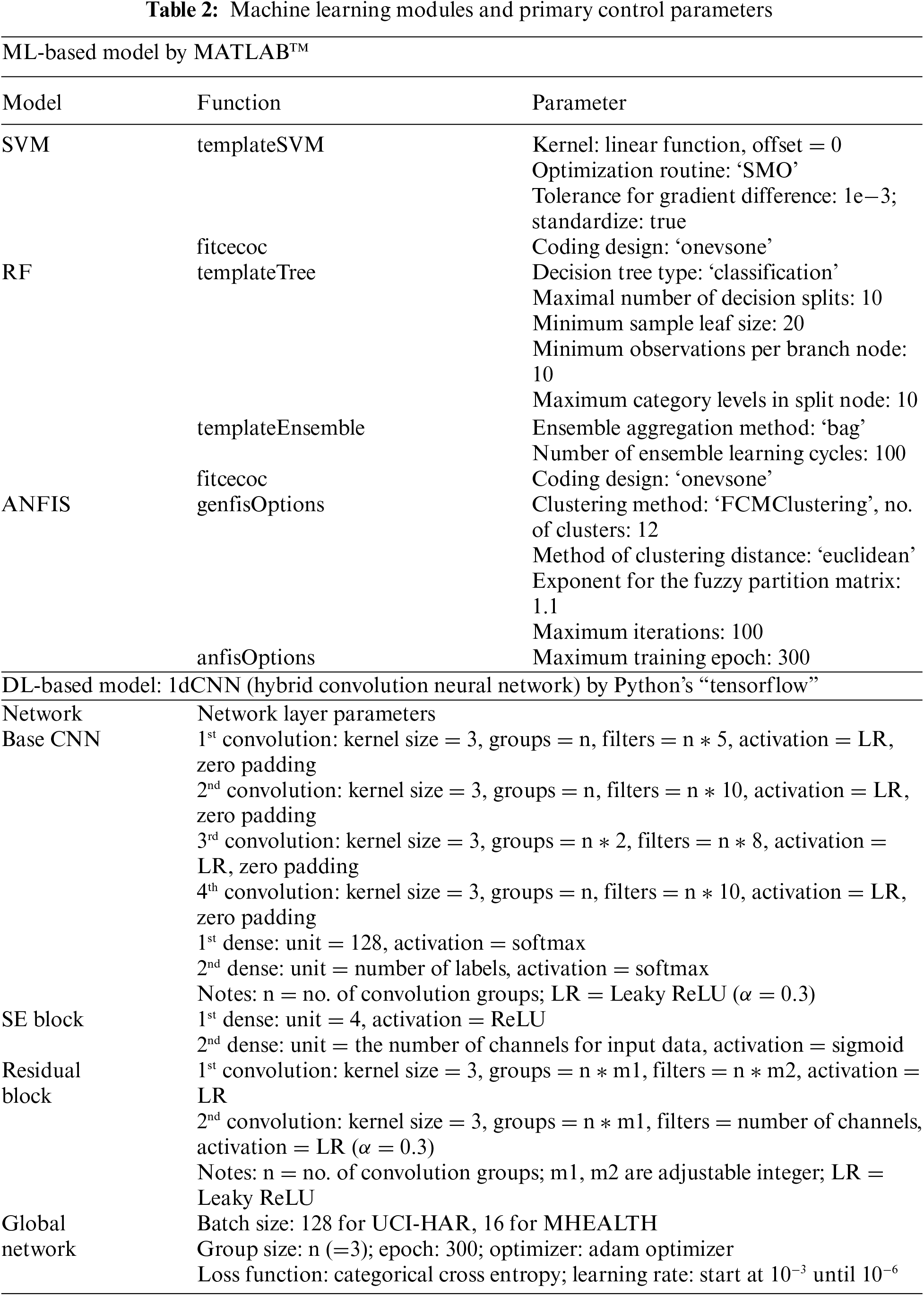
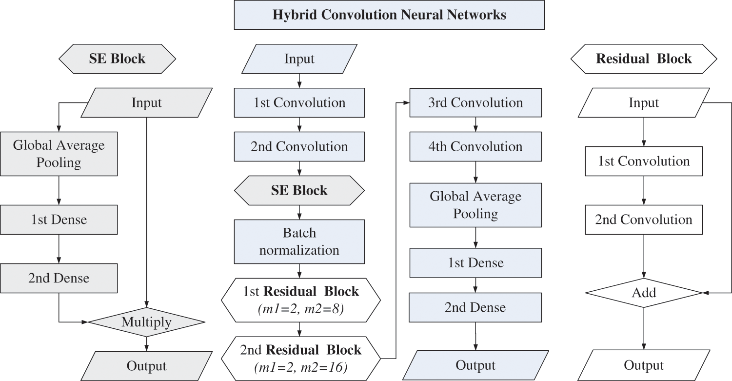
Figure 1: Architecture of one-dimensional convolutional neural network (1dCNN) model

A. Support vector machine (SVM)—The SVM method mathematically includes the allowable error variables in the objective functions, which presents the buffer range of partition boundaries in the high-dimensional domain. The method engages the error minimization principle to maximize the boundary between the two classes. The support vector on the boundary yields a formula to separate the classes for recognition. The computation applying a subset of training points to the support vectors can perform effective decision functions in high-dimensional spaces with efficient memory [21]. In computing, various kernel functions are recruited to simplify the transforming process of mapping features from complex boundaries to linear ones. This study adopted a linear kernel provided by “templateSVM” of MATLAB’s machine learning template for setting up the “fitcecoc” function. The primary parameters are shown in Table 2.

B. Random forest (RF)—The method of random forest (RF) drives ensemble learning sets by conducting multiple decision trees, which calculate information gains of conditional nodes (i.e., the branches of trees) to judge the possibility of class events and the most potential category is output for prediction [22]. In a stable RF model, the various learning sets can fit parallel without dependencies, and multiple weak learners can be integrated into a strong learner. The calculation involves weight regression for the loss function to improve the gradient of features and optimize weak learning in the model. A bootstrap aggregating (Bag) algorithm randomly generates subset trees for each sampling and averages the prediction results to enhance the RF model. The MATLAB’s templates, “templateTree” and “templateEnsemble”, were ensemble for setting up the “fitcecoc” function to create a strong learner by iteratively adding weak learners in this study. The primary parameters for RF’s “trees” are shown in Table 2.

C. Adaptive neural fuzzy inference system (ANFIS)—The ANFIS implements Sugeno-type FIS that uses a crisp set as the membership function (MF) of output classes for optimization and adaptability while applying the geometrical MFs due to data distribution pattern for the input features [23]. The crisp set consists of dependent coefficients of linear functions that will be adjusted with input features’ MFs for the neural network’s iterative fuzzification and defuzzification processes. The network contains clear control rules of fuzzy logic in the hidden layer, which can initialize proper parameters and train the parameters in iteration according to the rules [24]. However, MATLAB’s toolbox allows about 256 fuzzy logic rules for computing capacity at most, which limits the number of input features. We, therefore, employed fuzzy C-means clustering (FCM) methods [25] to identify the MFs of the FIS by organizing data samples into clusters for analysis. The FCM drives the number of clusters, the clustering exponent, and the distance metric in the input space to identify the premise MFs of the FIS structure for processing ANFIS. According to the assigned numbers of clusters, the clustering exponent and the distance metric compute the amount of fuzzy overlap between clusters, in which larger values indicate a greater degree of overlap, to partition the input space of features. Then, the clusters can be defined by selected MFs and the fuzzy logic rules can be created for all inputs. For an example of the m input features, each input can contain n clusters, and a Gauss-type MF defines each cluster; then, the FIS contains n fuzzy logic rules in which each rule as Eq. (1) can control m conditions with respect to the correspondent MFs of inputs for the output cluster. Due to MATLAB’s “anfis” function, we initialized FIS through “genfisOptions” and set up ANFIS’s learning epoch by “anfisOptions”. The important parameters are revealed in Table 2.

If [inputi]is [MFi−j] and … Then [output]is [cluster−outputj];i=1∼m,j=1∼n(1)

D. Hybrid convolution neural networks (CNNs)—We generated a one-dimensional CNN (1dCNN) model with hybrid CNNs, which involved SE and residual blocks in the CNN layers as shown in Fig. 1, to compare the efficiency of DL and ML methods in HAR. The necessary coefficients for modeling are shown in Table 2. Each input contains the same quantity of fragments for the DL methods, which differs from the feature data format for the ML methods. In the convolution layer, the CNN method drives different kernels for convolution and pooling operations that filter all inputs to extract possible features. The feature maps are integrated into a concatenate layer for advanced calculation in subsequent network layers. The “Conv1d” functions of Python’s “tensorflow” package were applied to the model for 1-D convolutions. The kernel’s initial weight was randomly assigned by the uniform Xavier initialization method [26,27]. Due to the architecture, we also grouped three-axis components of each physical quantity (e.g., accelerations) for parallel convolution [28]. The proposed model comprises two convolutional layers with a max pooling layer to construct a prototype of HAR for training data. An activation function “Leaky ReLU” in Eq. (2) was used in the convolutional layer, where a weight coefficient α = 0.3 in the study.

{f(x)=x,if x>0f(x)=αx,if x≤0(2)

The model was superposed by a batch normalization (BN) layer and SE block, which can normalize the fragment in a standard normal distribution and consistently adjust the weights of feature maps in the training process, respectively [29]. We added two residual blocks to avoid degradation and a global average pooling layer to produce the feature maps before full connection. We applied the activation function “softmax,” as shown in Eq. (3), in the fully connected layers to attain the label’s probability. The label with the highest probability value was recognized as the output.

softmax(x)=exi∑j=1nexj;i=1,2,3,…,n(3)

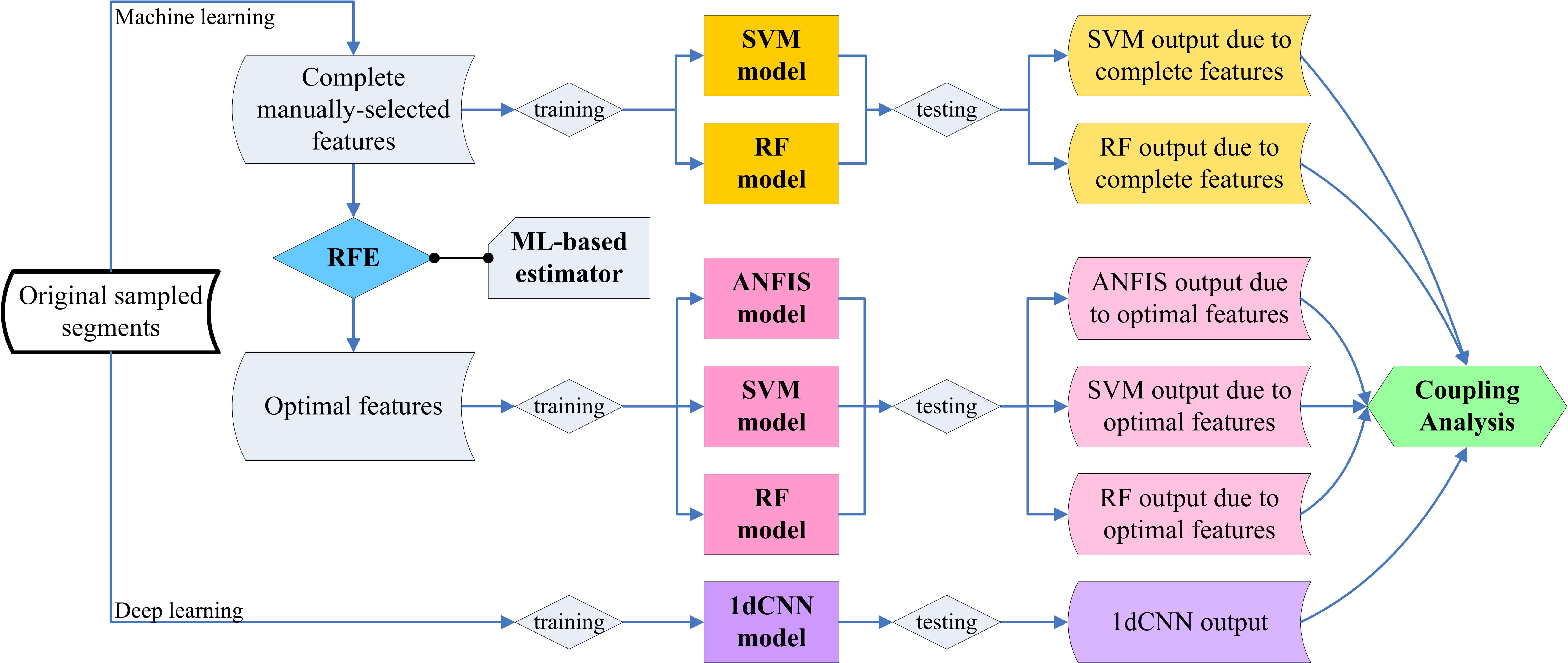
E. Recursive feature elimination (RFE)—The RFE method recursively estimates smaller sets of features to rank weights of the features and selects the optimal features for modeling [15]. To discover the number of optimal features, a cross-validation method is repeatedly combined with RFE’s ML-based estimator to score different feature subsets until the features with the best scores are collected [30]. With the estimator, the selected features are ranked by the features’ importance, and a small number of features are eliminated recursively per loop. The RFE process is detailed in Fig. 2. We employed the RFE and support vector classifier (SVC) from the Python-based scikit-learn library (known as the “sklearn” package) to explore the potential features for modeling in this study. The linear-kernel SVC is an SVM estimator of RFE for cross-validation. In this study, we applied RFE to compare the importance of features for each model, particularly for the ANFIS models that were restricted by the number of input features and fuzzy rules [31].

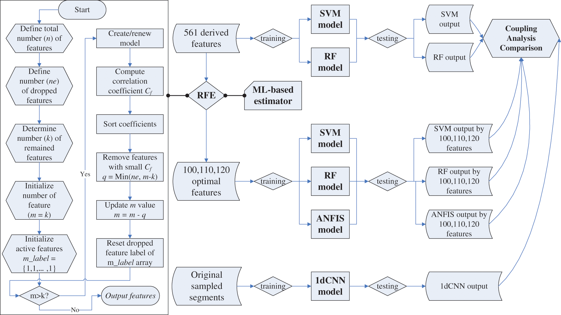
Figure 2: Coupling analysis framework including RFE process and three stages for evaluating the ML and DL models trained by UCI-HAR datasets

2.3 Coupling Analysis of Multiple Models

In the study, the UCI-HAR datasets, including manually selected features, were primarily substituted into the ML and DL models mentioned above for three-stage coupling analysis. The analysis flow chart is shown in Fig. 2. We first substituted all 561 features into the SVM and RF models for data training. The stage would verify the modeling with the previous studies. Then, we applied the RFE combining SVM estimator (RFE+SVM) to screen the optimal features and substituted them into proposed ML models (i.e., SVM, RF, ANFIS) for data training. We selected the groups of 75, 100, 110, 120, 130, 140, and 150 features, as referred in Table S2, and adopted the groups of 100, 110, and 120 features for satisfying ANFIS’s restrictions, including consuming time and computing capacity to conform the available number of features for model’s performance. Finally, we substituted the samples of original signal segments into the 1dCNN model for deep learning. The stages would discover the computation effectiveness of ML modeling, which selected features manually, and DL modeling, which extracted features automatically.

2.4 Comparative Modeling with MHEALTH and WISDM Open Datasets

Furthermore, the MHEALTH open dataset was used for comparative modeling with the UCI-HAR, while the WISDM open dataset was used to approve the modeling’ applicability. The MHEALTH measured three sensor nodes, different from one sensor on the waist for UCI-HAR, on the chest, ankle, and arm to collect three-axial vectors of acceleration, angular velocity, and magnetic field. The raw signals contained seven time-domain analytical features that FFT could convert to frequency-domain features. Due to the measured datasets, a raw segment with a sampling frequency of 50 Hz contained 128 timestamps with 50% overlap. Referring to UCI-HAR’s featuring and RFE process, we selected eight functions, including “mean”, “std”, “mad”, “max”, “min”, “energy”, “iqr”, and “kurtosis”, which are denoted in Table S3, to derive the features from each segment. Based on these functions, the analytical features in each domain could derive 168 features for modeling. Twelve activities: {standing, sitting, laying, walking, climbing stairs, bending waist, raising arm, crouching knee, cycling, jogging, running, jumping front and back} were labeled by {sta, sit, lay, walk, cs, bw, ra, ck, cycl, jog, run, jump} that contain the amount of data {480, 480, 480, 480, 480, 444, 460, 460, 480, 480, 480, 162}, respectively.

We then substituted the WISDM into the modeling, using 48 three-axis time-domain features derived by the eight functions above to explore the model’s applicability. The WISDM offered surveillance for 51 subjects with a smartwatch on hand and a smartphone in pocket to measure 18 lifestyle activities: {walking, jogging, climbing stairs, sitting, standing, typing, brushing teeth, eating soup, eating chips, eating pasta, drinking from cup, eating sandwich, kicking soccer ball, playing catch with tennis ball, dribbling basketball, writing, clapping, folding clothes}, which were labeled with prefix “label” orderly from 0 to 17. The smart phone and watch were embedded with an accelerometer and gyroscope for measurement. A measured segment contained 128 timestamps but with a frequency of 20 Hz, and 50% overlap between two segments. To simplify complicated data combination for application, we categorized four segment groups in comparison: (a) smartphone’s accelerometer and gyroscope, (b) smartwatch’s accelerometer and gyroscope, (c) accelerometers of smartphone and smartwatch, and (d) gyroscope of smartphone and smartwatch. The functions of derived features and the number of segments corresponding to the activity labels are detailed in Table S3 for reference.

We followed a portion ratio of 7:3 for training vs. testing groups based on label-oriented data training designed in the MHEALTH and WISDM; i.e., every subject’s dataset could be trained and tested while the testing group would not be trained. The design could be compared with the UCI-HAR by subject-oriented analysis (i.e., the subjects whose data were trained would not be tested). The training and testing processes above repeated the framework, as shown in Fig. 2, to generate the ML and DL models for coupling analysis. A confusion matrix with indicators, i.e., overall accuracy, recall, precision, and F1-score in one-vs.-all mode, evaluated the model’s efficacy.

3  Results

Four HAR models based on the methods, including SVM, RF, ANFIS, and hybrid CNNs, were trained by two databases for coupling analyses. The primary results regarding the UCI-HAR are demonstrated in the first three sub-sections. Consequently, the approaches regarding the comparative modeling due to the MHEALTH are exhibited for a comprehensive discussion.

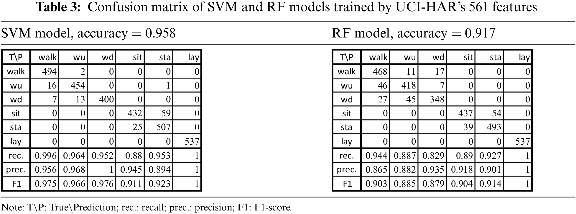
3.1 SVM and RF Models Trained by UCI-HAR’s 561 Features

The SVM and RF models trained by 561 features could reach overall accuracies of 95.8% and 91.7%, respectively. As shown in Table 3, the confusion matrixes reveal that the SVM model could recognize more activity patterns than the RF model. The SVM model could completely recognize a total of 400 and 537 walking downstairs and laying patterns (i.e., “wd” and “lay”), respectively; while the RF model worked excellently for the laying pattern. The past study approved the SVM’s results [12] using the multiclass SVM for UCI-HAR with approaches of overall accuracy at 96% for 2947 test patterns.

3.2 ANFIS, SVM, and RF Models Trained by UCI-HAR’s Optimal Features

The computing capacity of MATLABTM software limited the ANFIS models and could not contain all features in training. Therefore, we employed the RFE+SVM method to select 100, 110, and 120 features for training SVM, RF, and ANFIS models. The selected features are referred in Table S2. As a result, the overall accuracies of SVM, RF, and ANFIS models corresponding to 100 optimal features were 93.9%, 88.8%, and 89.8%, respectively, and that due to 110 and 120 features were {93.9%, 89.2%, 91.4%}, {94.6%, 89.5%, 90.5%}, respectively. Their confusion matrixes were detailed as shown in Table 4–parts Tables 4a–4c, in which various models trained by the same features displayed comparable accuracies between about 89% and 95%.

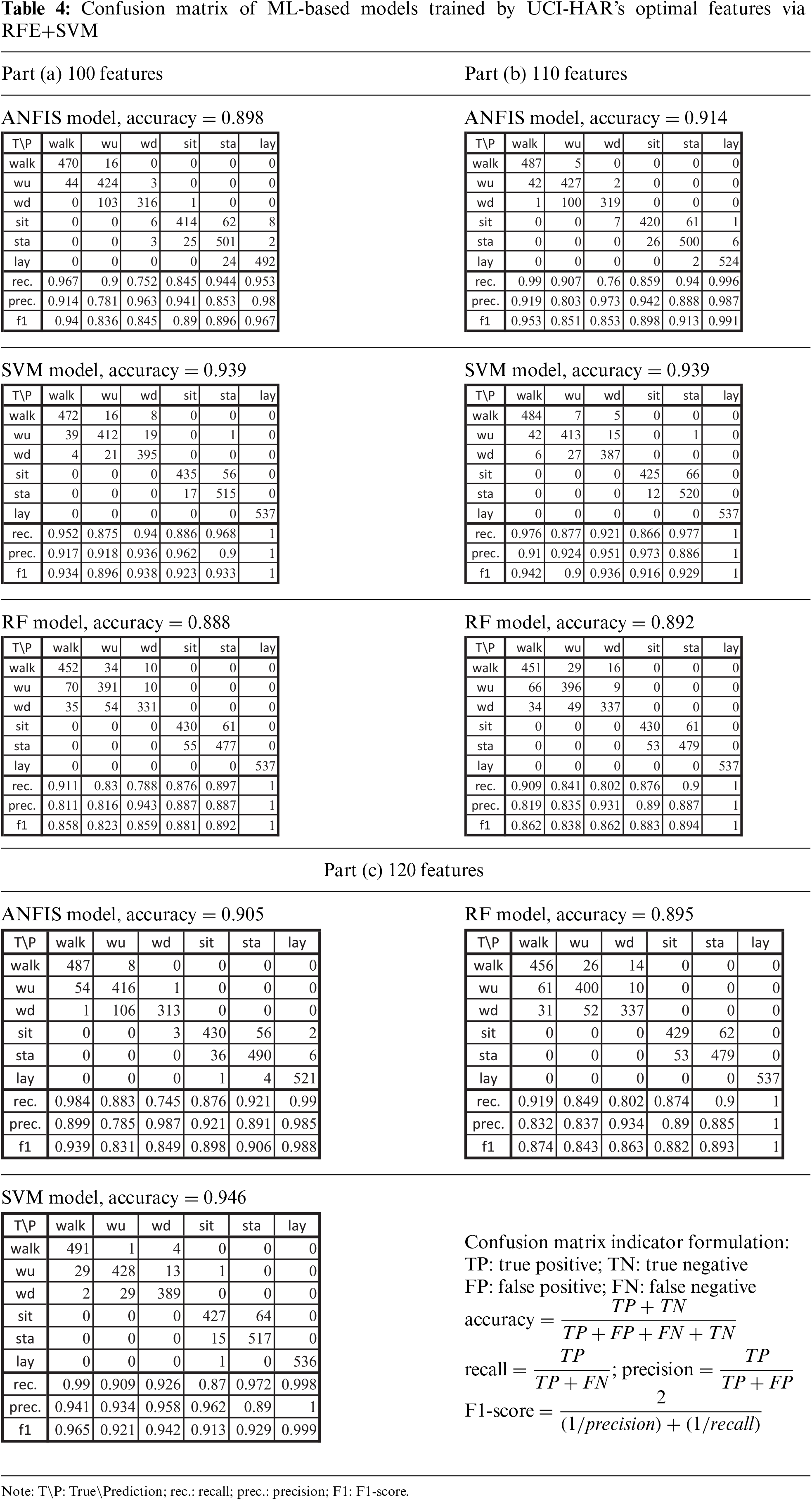
In general, three ML-based models could achieve an accuracy of over 89% by selected features, yet the SVM model performed better recognition than the RF and ANFIS models. SVM and RF models trained with 120 selected features were better than those trained with 100 and 110 features. Due to the confusion matrix, the laying patterns (i.e., “lay”) exhibit the most recognized activity since all models, excluding ANFIS by 100 features, could almost identify 537 patterns.

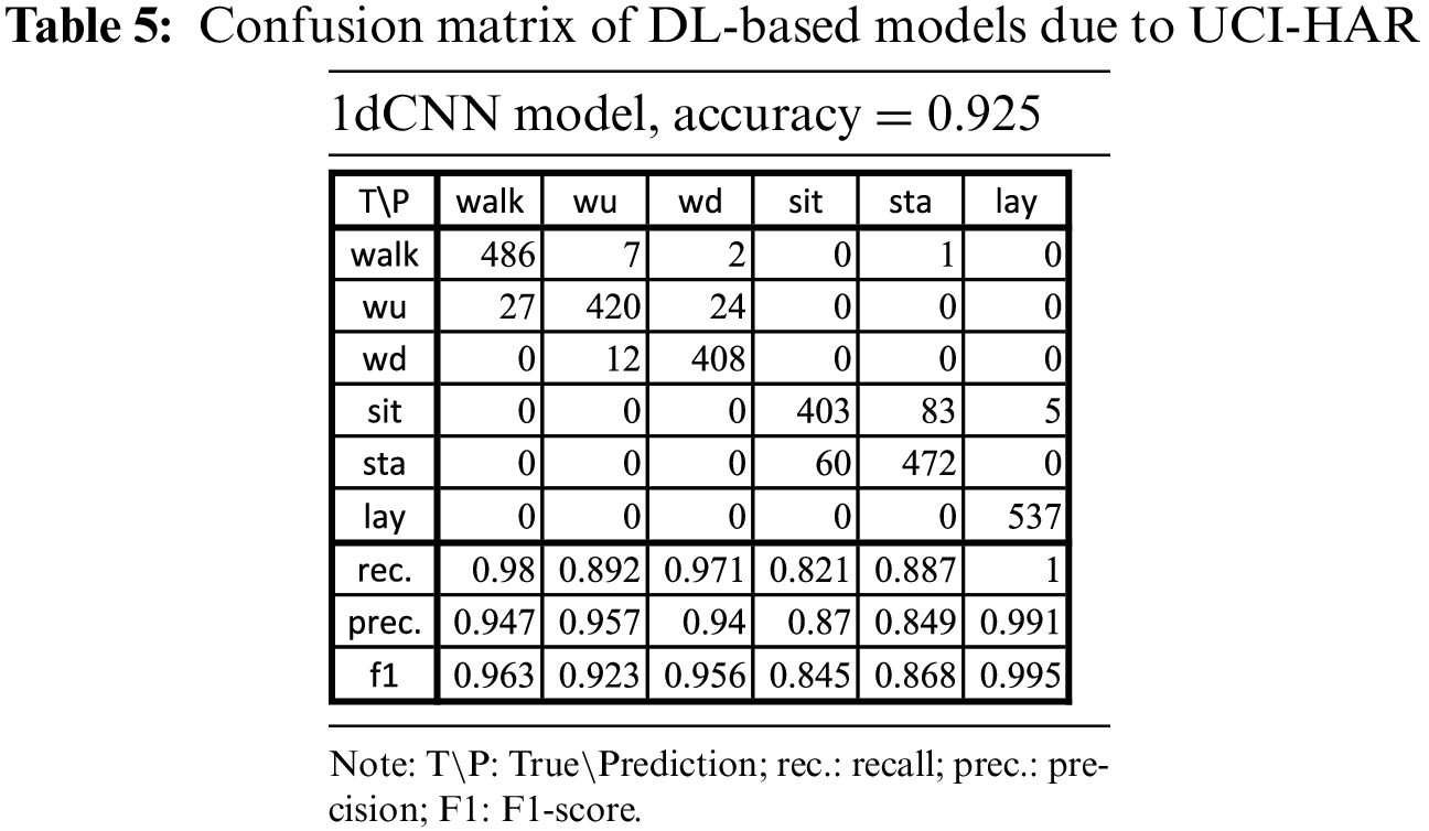
3.3 1dCNN Model by Deep Learning UCI-HAR Datasets

In comparison with previous ML models, we evaluated the proposed DL model 1dCNN, which was trained by the original datasets of the same subjects but without feature selection. The overall accuracy reached 92.5% due to the confusion matrix, as shown in Table 5.

3.4 DL and ML Models Trained by MHEALTH’s Features

Due to previous results, the ANFIS was not suitable for training with numerous features. For comparative modeling, we used MHEALTH’s original time-domain segments to train the 1dCNN model and adopted the features through RFE to train the RF, SVM, and ANFIS models. The indicators evaluated the DL and ML models, i.e., overall accuracy, recall, precision, and F1-score, as shown in Table 6.

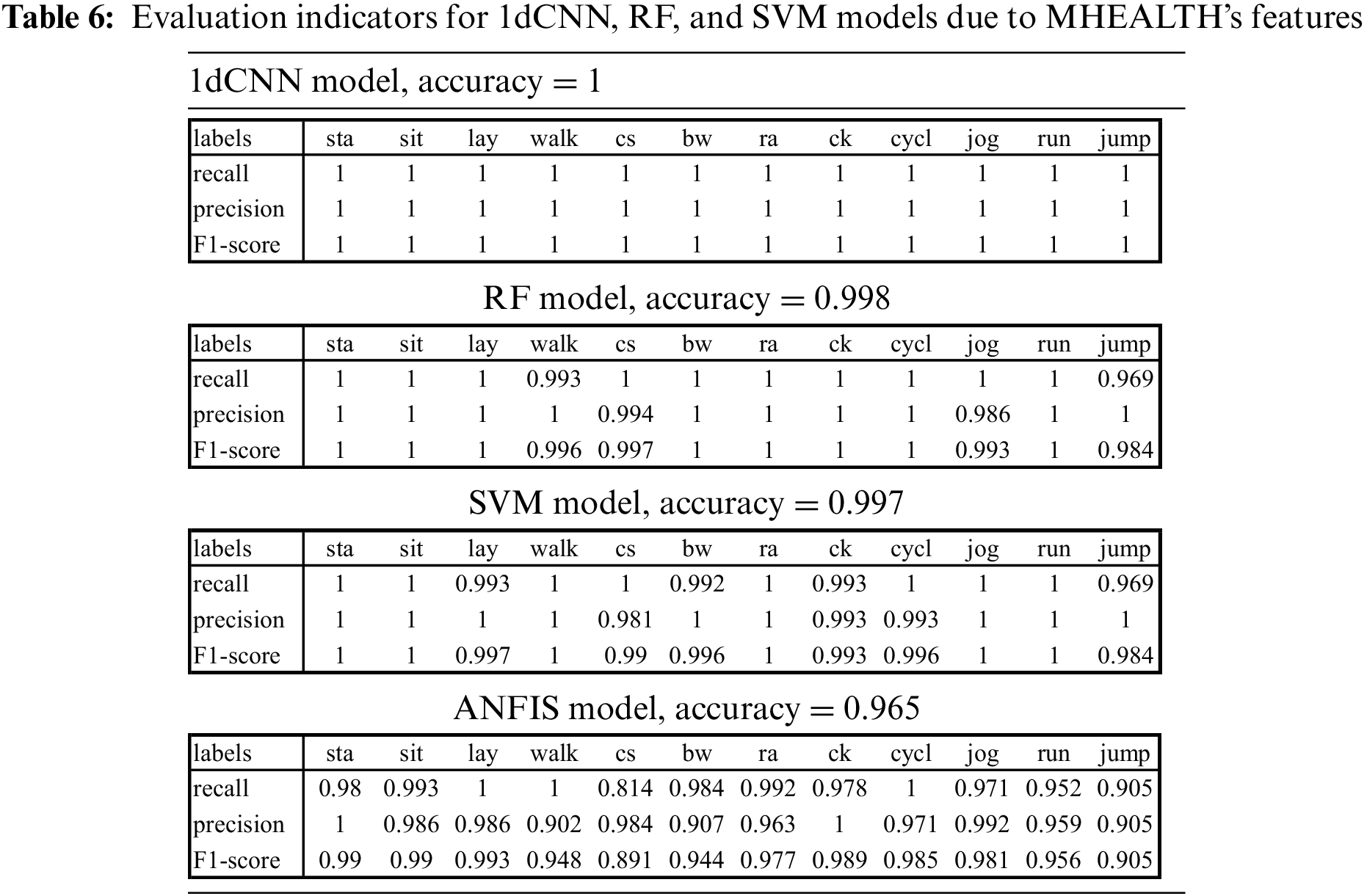
The 1dCNN model achieved an overall accuracy of 100% for the 12 labels validated by the previous study [11], i.e., all activities were perfectly recognized. Considering 336 features derived from eight types of functions in time and frequency domains for training the ML models, the RF and SVM models reached overall accuracies of 99.8% and 99.7%, respectively. We further explored the performance using the single-functioned feature to train the SVM model. The accuracies corresponding to {mean, std, mad, max, min, energy, iqr, kurtosis} were {99.6%, 99.6%, 95.2%, 91.7%, 99.6%, 98.0%, 99.9%, 91.8%}, respectively. We experienced that the features derived by specific functions could reach a good accuracy over 91.7%. Consequently, we used 84 time-domain features derived by mean, std, min, and iqr functions, which obtained excellent performance for SVM, to train the ANFIS model and achieved an accuracy of 96.5%. The results of comparative modeling approved the coupling analysis framework with proper feature selection.

Each algorithm is applicable in some fields but is probably limited in others. We proposed the coupling analysis framework that recruited the UCI-HAR and MHEALTH open data to train the HAR models based on four classic ML and DL methods for comparison. The modeling process could concurrently evaluate and provide the comparative models with the best approaches as a reference for the implementation of AI-enabled healthcare systems.

4  Discussions

This study developed a coupling analysis framework to build the HAR models by exploring the methods of ANFIS, SVM, RF, and hybrid CNN sequentially the representative techniques for each decade in the past four decades. The framework can generate suitable models with efficient modeling process and adapt to AI-enabled applications. After coupling analysis, the efficacies of four HAR models corresponding to the open databases were compared. The limitations, findings, comparisons, and applications are discussed below.

4.1 Limitations

We employed MATLAB’s neuro-fuzzy designer toolbox to establish the ANFIS models, which were limited by the software’s calculation capability. If UCI-HAR’s 561 features for 7532 data pairs were trained, the array size would be 226.3 GB, which exceeds MATLAB’s maximum preference. The RFE method was then considered for feature selection to reduce computing resources. In addition, a DL model usually requires extra GPU to improve computing performance. We therefore added a video card with chips of NVidia GeForce RTX 2070 plus 8 GB RAM on the desktop computer embedded with Intel® Core™ i7-7700 CPU @ 3.60 GHz and 64 GB RAM.

4.2 Findings

All of the suggested methods could achieve an overall accuracy of 90%, which is acceptable for HAR, by selecting the proper features for the ML-based models or designing the network architecture for the DL-based models. We were interested in evaluating the model’s efficacy.

(1) Evaluating optimal features for improving the model’s efficacy. Proper feature selection could improve the model’s efficacy in machine learning for clinical applications on disease prediction [32]. With UCI-HAR datasets, we compared the ML-based models trained by three sets of 100, 110, and 120 features, as shown in Table 4 for the study. The SVM, RF, and ANFIS models could attain about 90% accuracy without using 561 features. The 110 features were enough for ANFIS to obtain acceptable accuracy (91.4%) with efficient computing resources for the proposed models in the UCI-HAR case. The SVM model’s best accuracy (94.6%) was only 1.2% to 95.8% of the model trained by 561 features. For MHEALTH datasets, we experienced poor features, causing SVM’s difficulty separating complex dimensional spaces during training. With the chosen 336 features, the SVM and RF models achieved higher than 99% accuracy. Meanwhile, the ANFIS model was improved to reach an accuracy of around 97%.

(2) Evaluating time efficiency of iteration and non-iteration models. From the machine learning aspect, the non-iterative algorithms benefit from efficient calculation for the non-NN-based models. In contrast, the iterative algorithms are computationally stable for the NN-based models [33]. For the UCI-HAR case, the study took about 20–25 s to train non-iterative SVM and RF models with 561 features. In addition, the iterative RFE+SVM method spent 42 min selecting 110 optimal features, which reduced training time to less than 12 s for SVM and RF models. However, the iterative ANFIS model required more than 5 h for training in 300 epochs, which initially created the FIS with these features in clustering by at most 100 iterations. All well-trained models could complete recognition for a feature set in a few millisecond. For deep learning, the 1dCNN model took about three to four minutes for data training in 300 epochs. In general, four models can achieve at least 90% of accuracy. If the quality of HAR data were good, then the non-iterative algorithms would be suggested to train the model for efficient, time-consuming tasks. However, when analyzing the complex activities that caused ambiguous data quality, the iterative algorithms would be helpful to explore proper features to improve the model’s recognition capability.

(3) Evaluating featuring modes due to DL-based and ML-based models. The DL-based models were known to extract concealed features in training while the ML models requested selecting possible features for learning. With UCI-HAR’s features, each model’s average accuracies are shown in Fig. 3 and Table 4. The DL-based 1dCNN model reached an accuracy of about 93%, slightly higher than the ML-based RF and ANFIS models (approximately 90%) but lower than ML-based SVM models (about 95%). Our previous study suggested multiple heterogeneous inputs in hybrid CNNs with hierarchical modeling to reach an accuracy of 96% for UCI-HAR [34]. The recent study proposed a DL-based model, which coupled optimal features due to data pre-processing with deep convolutional neural network (DCNN) and long short-term memory (LSTM) methods for data training, could achieve an overall accuracy of 99.9% for UCI-HAR [35]. Furthermore, the innovative HAR technique could drive the multi-head CNN with convolution block attention module and LSTM to recognize multi-level features with the time-sensitive multi-source sensor information [36]. Besides, the advanced method of fusion features could concatenate the features derived for the conventional ML model with the DL feature maps in the CNN structure [37]. The studies approved that manual and automatic operations can help extract appropriate features for training the ML and DL models.

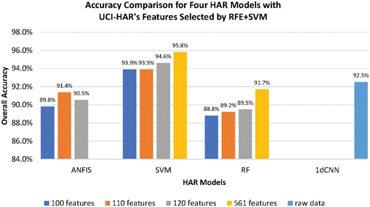
Figure 3: Overall accuracies of the ML and DL models trained by the UCI-HAR database

(4) Evaluating the model’s accuracy according to RFE’s estimator. Redundant features usually increase dimensional complexity to reduce machine learning effectiveness. The RFE was known to remain a subset of the most relevant features for a dataset by incorporating the proper ML model as an estimator to repeatedly classify all features through cross-validation and regression [38]. In regression, all features were ranked by calculating the importance scores, e.g., information gain; then, the lower-ranked features standing for the most irrelevant features in each cross-validation epoch could be eliminated recursively [39]. Machine learning has challenges for HAR in irregular movements implying specific features of high dimensionality [40]. We were interested in the performance of the selected features due to RFE’s ML estimators. For the UCI-HAR case, we used RF as RFE’s estimator (i.e., RFE+RF) to select features for comparison with RFE+SVM. The optimal features due to RFE+RF, as referred to in Table S4, were partially different from that of RFE+SVM. The accuracies of the RF model due to the feature sets by RFE+RF, as shown in Fig. 4, were approximately 1% better than the feature sets by RFE+SVM. The accuracies of SVM models due to the 100, 110, and 120 optimal features of RFE+RF were similar to the feature sets of RFE+SVM. However, the SVM models trained by 130, 140, and 150 features based on RFE+RF could reach an accuracy of around 96%, the same as using 561 features. In this case, the SVM models performed with better accuracy than the RF models due to the features selected by both RFE methods.

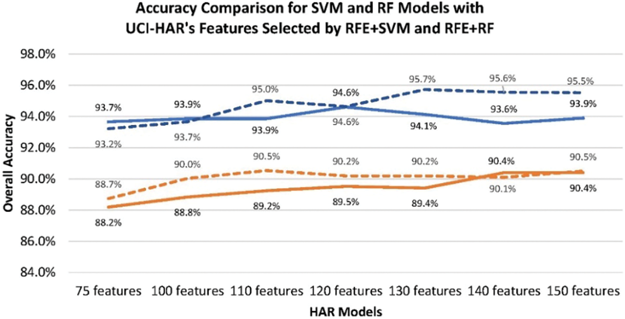
Figure 4: Accuracies of the SVM and RF models due to UCI-HAR’s features selected by RFE

(5) Evaluating comparative analyses with UCI-HAR and MHEALTH datasets. The UCI-HAR study was initially considered a subject-oriented analysis that split the subjects into training and testing groups (i.e., 7:3) to recognize six labels. For the MHEALTH case that provided few subjects, we proposed a label-oriented analysis, i.e., split all features of each label into the training and testing groups randomly, to ensure the model could learn the subject’s habitual motions and a perfect accuracy (i.e., 100%) was obtained by 1dCNN. If the MHEALTH trained the 1dCNN model with subject-oriented analysis (i.e., 7 subjects for training and 3 subjects for testing), the overall accuracy was 0.9. With the same analysis for the SVM and RF models, the accuracies due to MHEALTH’s selected features were 0.878 and 0.953, respectively. Therefore, we adopted label-oriented analysis for the 1dCNN modeling with UCI-HAR. The overall accuracy was improved to 0.979. Similarly, the accuracies of the ANFIS, SVM, and RF models trained by the 100 optimal features were increased to 0.954, 0.975, and 0.963, respectively, as shown in Table S5.

4.3 Comparisons

We initially considered merging the UCI-HAR and MHEALTH datasets labeled the same activities for advanced analysis. However, the collected datasets of the two projects could not be unified since their subjects wore the sensors at different locations. The models trained by the UCI-HAR and MHEALTH datasets could not identify each other’s features. For comparing various data measurements, we considered the subject-and label-oriented analyses for the modeling with both datasets. In comparison, the ANFIS model provides adaptive interpretation capabilities to infer complex patterns for nonlinear relationships, but it remains a challenge in computation for the curse of dimensionality [41]. The SVM model benefits from calculating high-dimensional data but is quite sensitive to noise and outliers. In contrast, the RF model can compute various data types and eliminate outliers and missing values. Still, it is unsuitable for inferring a variable’s significance [42]. The CNN model automatically filters underlying features to deliver high accuracy in recognition tasks but requires more hardware capacity for large network size and complexity [43]. In practice, every learning algorithm is available for implementation in a relatively suitable field to perform good results. We suggested a personalized healthcare program for the HAR applications that can collect universalized datasets from the subjects to ensure reliable HAR quality. The users can choose the appropriate model based on the requirement level.

4.4 Applications

We finally evaluated the framework’s robustness and versatility by applying the proposed coupling analysis to a WISDM database, which offered lifestyle surveillance for 51 subjects with a smartwatch on hand and a smartphone in pocket to measure 18 activities. Our approaches, as shown in Table S6, yielded 91.4% and 87.3% accuracy for the 1dCNN and RF models, respectively, trained by the datasets due to the phone’s and watch’s accelerometers; conversely, 83.1% and 72.4% for the gyroscopes. The framework’s robustness was confirmed by a recent study indicating that DL-based convolutional LSTM and ML-based RF models achieved accuracies of 84.1% and 61.1% for the smartwatch, respectively, as well as 84.9% and 75.4% for the smartphone [44].

The framework would be produced as the modular package via Python’s “Model.save” functionality or MATLAB’s “library compiler” toolbox. The packages can be adapted to the artificial intelligence of things (AIoT) system developed in our previous study for physiotherapy programs to track rehabilitation motions [45]. Due to an exercise guideline for rehabilitation management in healthcare services, the patient used to rehab the injured limbs with simple actions. The modeling with label-oriented analysis that trains a personalized model to recognize the subject’s activities can be practically utilized to track whether the patient obeys the guideline. For example, the subject can easily wear bracelets to collect signals of specified rehab exercises. The personal HAR model of a surveillance system can be pre-trained within the framework. Then, the exercise labels can be quickly recognized, and feedback can be given when receiving the signals. The results can be displayed on the real-time dashboard for advanced healthcare management.

The above discussions revealed four AI-available HAR models in detail for data training on the classic ML and DL methods. The well-trained models could accomplish recognition for a set of hundred features around a few milliseconds. The performance metrics were compared with previous studies, as shown in Table S7. Past studies have usually applied wearable sensors for HAR applications in daily activity, self-harming, sleep management, and physical manipulation [46]. Based on the advantage of the coupling analysis process in testing three HAR open databases, the framework can discover proper features for the ML methods and involve effective layers in the DL structures for the diverse HAR models with adaptability to the above applications in the real world. The process can also derive the analytical features with comprehensive data preprocessing and training due to the datasets for reproducing the HAR models with computational efficiency. The proposed models were expandable for AI-enabled health promotion and management, e.g., incorporating AIoT in rehabilitation and self-fitness programs to utilize the HAR functionality for an advanced surveillance and healthcare system.

5  Conclusion

A coupling analysis framework of multiple HAR models investigated the ML and DL methods with the proper featuring process to attain good performance. The UCI-HAR was first employed to train the proposed models through the conventional ML and DL algorithms, including SVM, RF, ANFIS, and 1dCNN. Besides, the RFE method was applied to eliminate the features recursively from the datasets and retain the optimal features for data training. The MHEALTH was then recruited to follow the modeling process for comparison. The WISDM was finally applied to approve the framework’s robustness and versatility.

For the UCI-HAR, the SVM and RF models achieved accuracy at about 95% and 90%, respectively, with efficient computing time. The ANFIS model restricted to the number of fuzzy logic rules could reach 91% with a proper clustering process and RFE operations. Compared with the ML-based model, the 1dCNN model stably filtered the raw datasets through convolution operations to perform an accuracy of around 93%. Furthermore, the MHEALTH datasets were recruited using the same process to train the ML and DL models for comparison. With RFE, 336 features were adopted for ML-based modeling, in which the accuracy of SVM and RF models could achieve more than 99%. By selecting the 84 time-domain features, the ANFIS model could reach an accuracy of 96.5%. The DL-based 1dCNN model could perform a perfect accuracy of 100%. The comparative modeling consequently approved the feasibility of the proposed coupling analysis framework. Finally, for the WISDM, the ML-based and DL-based models could reach 87.3% and 91.4% accuracy, respectively, due to data measured by the accelerometers of the smartphone and smartwatch.

In conclusion, the proposed HAR models, which performed well, were suitable for AI-enabled applications. We finally contributed a coupling analysis framework with the computing processes of four HAR models based on classic machine learning methods. The analysis is flexible in exploring more novel datasets, which measure complex signals, images, or videos in various dimensions, for creating diverse HAR models in the extended study. The model can be modularly adapted to AI-enabled home healthcare services for health management by tracking daily activity, self-harming, physical manipulation, etc. The framework will be integrated with emerging technologies in the future, e.g., joining artificial intelligence of things (AIoT) with personalized HAR functionality on smart medicine, self-fitness, and rehabilitation programs for health promotion challenges.

Acknowledgement: The authors extend their gratitude to Brady Ling, a senior student at the Foster School of Business, University of Washington at Seattle, USA, for his hard work and commitment as an English volunteer editorial reviewer.

Funding Statement: This research was funded by the National Science and Technology Council, Taiwan (Grant No. NSTC 112-2121-M-039-001) and by China Medical University (Grant No. CMU112-MF-79).

Author Contributions: Y. -C. Lai conducted data analysis and implemented machine learning techniques in the study. S. -Y. Chiang provided expert guidance on the application of machine learning methods. Y. -C. Kan offered insights on data pre-processing for modelling processes. H. -C. Lin, as the corresponding author, conceived the study, contributed to its investigation, development, and coordination, and wrote the original draft. All authors have reviewed and approved the final version of the manuscript for publication.

Availability of Data and Materials: This study used the UCI-HAR, the MHEALTH, and the WISDM open databases that are available online–https://archive.ics.uci.edu/dataset/240/human+activity+recognition+using+smartphones. https://archive.ics.uci.edu/dataset/319/mhealth+dataset. https://archive.ics.uci.edu/dataset/507/wisdm+smartphone+and+smartwatch+activity+and+biometrics+dataset.

Conflicts of Interest: The authors declare they have no conflicts of interest to report regarding the present study.

Supplementary Materials: The supplementary material is available online at https://doi.org/10.32604/cmc.2024.050376.

References

1. N. Gupta, S. K. Gupta, R. K. Pathak, V. Jain, P. Rashidi and J. S. Suri, “Human activity recognition in artificial intelligence framework: A narrative review,” Artif. Intell. Rev., vol. 55, no. 6, pp. 4755–4808, 2022. doi: 10.1007/s10462-021-10116-x. [Google Scholar] [PubMed] [CrossRef]

2. L. Ling et al., “An efficient method for identifying lower limb behavior intentions based on surface electromyography,” Comput. Mater. Contin., vol. 77, no. 3, pp. 2771–2790, 2023. doi: 10.32604/cmc.2023.043383. [Google Scholar] [CrossRef]

3. G. Bhola and D. K. Vishwakarma, “A review of vision-based indoor HAR: State-of-the-art, challenges, and future prospects,” Multimed. Tools Appl., vol. 83, no. 1, pp. 1965–2005, 2024. doi: 10.1007/s11042-023-15443-5. [Google Scholar] [PubMed] [CrossRef]

4. Z. Meng et al., “Recent progress in sensing and computing techniques for human activity recognition and motion analysis,” Electronics, vol. 9, no. 9, pp. 1357, 2020. doi: 10.3390/electronics9091357. [Google Scholar] [CrossRef]

5. S. B. Kotsiantis, “Supervised machine learning: A review of classification techniques,” Information, vol. 31, pp. 249–268, 2007. [Google Scholar]

6. D. Anguita, A. Ghio, L. Oneto, X. Parra, and J. L. Reyes-Ortiz, “Human activity recognition on smartphones using a multiclass hardware-friendly support vector machine,” in Lecture Notes in Computer Science (LNCS), Berlin, Heidelberg: Springer, 2012, vol. 7657, pp. 216–223. 10.1007/978-3-642-35395-6_30. [Google Scholar] [CrossRef]

7. F. Attal, S. Mohammed, M. Dedabrishvili, F. Chamroukhi, L. Oukhellou and Y. Amirat, “Physical human activity recognition using wearable sensors,” Sensors, vol. 15, no. 12, pp. 31314–31338, 2015. doi: 10.3390/s151229858. [Google Scholar] [PubMed] [CrossRef]

8. D. Karaboga and E. Kaya, “Adaptive network based fuzzy inference system (ANFIS) training approaches: A comprehensive survey,” Artif. Intell. Rev., vol. 52, no. 4, pp. 2263–2293, 2019. doi: 10.1007/s10462-017-9610-2. [Google Scholar] [CrossRef]

9. O. S. Ajani and H. El-Hussieny, “An ANFIS-based human activity recognition using IMU sensor fusion,” presented at the 2019 Novel Intell. Lead. Emerg. Sci. Conf. (NILESGiza, Egypt, 2019, pp. 34–37. doi: 10.1109/NILES.2019.8909289. [Google Scholar] [CrossRef]

10. Y. LeCun, Y. Bengio, and G. Hinton, “Deep learning,” Nature, vol. 521, no. 7553, pp. 436–444, 2015. doi: 10.1038/nature14539. [Google Scholar] [PubMed] [CrossRef]

11. M. Gholamrezaii and S. M. T. Al Modarresi, “A time-efficient convolutional neural network model in human activity recognition,” Multimed. Tools Appl., vol. 80, no. 13, pp. 19361–19376, 2021. doi: 10.1007/s11042-020-10435-1. [Google Scholar] [CrossRef]

12. D. Anguita, A. Ghio, L. Oneto, X. Parra Perez, and J. L. Reyes-Ortiz, “A public domain dataset for human activity recognition using smartphones,” presented at the Eur. Symp. Artif. Neural Netw., Comput. Intell. Mach. Learn. (ESANN 2013Bruges, Belgium, Apr. 2013, pp. 24–26. [Google Scholar]

13. O. Banos et al., “Design, implementation and validation of a novel open framework for agile development of mobile health applications,” Biomed. Eng., vol. 14, no. 2, pp. 1–20, 2015. doi: 10.1186/1475-925X-14-S2-S6. [Google Scholar] [PubMed] [CrossRef]

14. G. Weiss, “WISDM Smartphone and Smartwatch Activity and Biometrics Dataset,” in UCI Machine Learning Repository, Irvine, California, USA: UCI Donald Bren School of Information & Computer Sciences, 2019. doi: 10.24432/C5HK59. [Google Scholar] [CrossRef]

15. A. Jović, K. Brkić, and N. Bogunović, “A review of feature selection methods with applications,” presented at the 2015 38th Int. Convent. Inf. Commun. Technol., Electron. Microelectron. (MIPROOpatija, Croatia, May 25–29, 2015. doi: 10.1109/MIPRO.2015.7160458. [Google Scholar] [CrossRef]

16. G. Chandrashekar and F. Sahin, “A survey on feature selection methods,” Comput. Electr. Eng., vol. 40, no. 1, pp. 16–28, 2014. doi: 10.1016/j.compeleceng.2013.11.024. [Google Scholar] [CrossRef]

17. H. Jeon and S. Oh, “Hybrid-recursive feature elimination for efficient feature selection,” Appl. Sci., vol. 10, no. 9, pp. 3211, 2020. doi: 10.3390/app10093211. [Google Scholar] [CrossRef]

18. M. Islam, S. Nooruddin, F. Karray, and G. Muhammad, “Human activity recognition using tools of convolutional neural networks: A state of the art review, data sets, challenges, and future prospects,” Comput. Biol. Med., vol. 149, pp. 106060, 2022. doi: 10.1016/j.compbiomed.2022.106060. [Google Scholar] [PubMed] [CrossRef]

19. K. He, X. Zhang, S. Ren, and J. Sun, “Deep residual learning for image recognition,” presented at the 2016 IEEE Conf. Comput. Vis. Pattern Recognit. (CVPRLas Vegas, NV, USA, Jun. 27–30, 2016, pp. 770–778. doi: 10.1109/CVPR.2016.90. [Google Scholar] [CrossRef]

20. J. Hu, L. Shen, and G. Sun, “Squeeze-and-excitation networks,” presented at the IEEE Conf. Comput. Vis. Pattern Recognit. (CVPRSalt Lake City, UT, USA, Jun. 19-21, 2018. [Google Scholar]

21. A. Ukil, “Support vector machine,” in Intelligent Systems and Signal Processing in Power Engineering. Power Systems (POWSYS), Berlin, Heidelberg, Germany: Springer, 2007, pp. 161–226. 10.1007/978-3-540-73170-2_4. [Google Scholar] [CrossRef]

22. M. Belgiu and L. Drăguţ, “Random forest in remote sensing: A review of applications and future directions,” ISPRS J. Photogramm. Remote Sens., vol. 114, pp. 24–31, 2016. doi: 10.1016/j.isprsjprs.2016.01.011. [Google Scholar] [CrossRef]

23. M. Golosovskiy, A. Bogomolov, and M. Balandov, “Algorithm for configuring sugeno-type fuzzy inference systems based on the nearest neighbor method for use in cyber-physical systems,” in Cyber-Phys. Syst.: Intell. Models Algorithms. Stud. Syst., Decis. Control (SSDC), Switzerland, Cham, Springer, 2022, vol. 417, pp. 83–97. doi: 10.1007/978-3-030-95116-0_7. [Google Scholar] [CrossRef]

24. A. Senthilselvi, J. S. Duela, R. Prabavathi, and D. Sara, “Performance evaluation of adaptive neuro fuzzy system (ANFIS) over fuzzy inference system (FIS) with optimization algorithm in de-noising of images from salt and pepper noise,” J. Ambient Intell. Hum. Comput., vol. 52, no. 12, pp. 1–6, 2021. doi: 10.1007/s12652-021-03024-z. [Google Scholar] [CrossRef]

25. K. Benmouiza and A. Cheknane, “Clustered ANFIS network using fuzzy c-means, subtractive clustering, and grid partitioning for hourly solar radiation forecasting,” Theor. Appl. Climatol., vol. 137, no. 1–2, pp. 31–43, 2019. doi: 10.1007/s00704-018-2576-4. [Google Scholar] [CrossRef]

26. H. Zhang, L. Feng, X. Zhang, Y. Yang, and J. Li, “Necessary conditions for convergence of CNNs and initialization of convolution kernels,” Digit. Signal Process., vol. 123, no. 4, pp. 103397, 2022. doi: 10.1016/j.dsp.2022.103397. [Google Scholar] [CrossRef]

27. X. Glorot and Y. Bengio, “Understanding the difficulty of training deep feedforward neural networks,” presented at the 13th Int. Conf. Artif. Intell. Stat., Sardinia, Italy, May 13–15, 2010. [Google Scholar]

28. X. Wang, M. Kan, S. Shan, and X. Chen, “Fully learnable group convolution for acceleration of deep neural networks,” presented at the 2019 IEEE/CVF Conf. Comput. Vis. Pattern Recognit. (CVPRLong Beach, CA, USA, Jun. 15–20, 2019. doi: 10.1109/CVPR.2019.00926. [Google Scholar] [CrossRef]

29. S. Ioffe and C. Szegedy, “Batch normalization: Accelerating deep network training by reducing internal covariate shift,” presented at the 32nd Int. Conf. Mach. Learn. (ICMLLille, France, Jul. 6–11, 2015. doi: 10.48550/arXiv.1502.03167. [Google Scholar] [CrossRef]

30. X. Lin et al., “A support vector machine-recursive feature elimination feature selection method based on artificial contrast variables and mutual information,” J. Chromatogr. B, vol. 910, no. 1, pp. 149–155, 2012. doi: 10.1016/j.jchromb.2012.05.020. [Google Scholar] [PubMed] [CrossRef]

31. G. Apicella, G. D’Aniello, G. Fortino, M. Gaeta, R. Gravina and L. G. Tramuto, “An adaptive neuro-fuzzy approach for activity recognition in situation-aware wearable systems,” presented at the 2022 IEEE 3rd Int. Conf. Human-Mach. Syst. (ICHMSOrlando, FL, USA, Nov. 17–19, 2022. doi: 10.1109/ICHMS56717.2022.9980773. [Google Scholar] [CrossRef]

32. T. Vivekanandan and N. C. S. N. Iyengar, “Optimal feature selection using a modified differential evolution algorithm and its effectiveness for prediction of heart disease,” Comput. Biol. Med., vol. 90, no. 1, pp. 125–136, 2017. doi: 10.1016/j.compbiomed.2017.09.011. [Google Scholar] [PubMed] [CrossRef]

33. O. E. Mountassir, B. G. Stewart, A. J. Reid, and S. G. McMeekin, “Quantification of the performance of iterative and non-iterative computational methods of locating partial discharges using RF measurement techniques,” Electr. Power Syst. Res., vol. 143, no. 3, pp. 110–120, 2017. doi: 10.1016/j.epsr.2016.10.036. [Google Scholar] [CrossRef]

34. Y. C. Lai, Y. C. Kan, K. C. Hsu, and H. C. Lin, “Multiple inputs modeling of hybrid convolutional neural networks for human activity recognition,” Biomed. Signal Process. Control, vol. 92, no. 9, pp. 106034, 2024. doi: 10.1016/j.bspc.2024.106034. [Google Scholar] [CrossRef]

35. S. Jameer and H. Syed, “A DCNN-LSTM based human activity recognition by mobile and wearable sensor networks,” Alex. Eng. J., vol. 80, no. 1, pp. 542–552, 2023. doi: 10.1016/j.aej.2023.09.013. [Google Scholar] [CrossRef]

36. M. Islam, S. Nooruddin, F. Karray, and G. Muhammad, “Multi-level feature fusion for multimodal human activity recognition in Internet of Healthcare Things,” Inf. Fusion, vol. 94, no. 12, pp. 17–31, 2023. doi: 10.1016/j.inffus.2023.01.015. [Google Scholar] [CrossRef]

37. D. Thakur and S. Biswas, “Feature fusion using deep learning for smartphone based human activity recognition,” Int. J. Inf. Tecnol., vol. 13, no. 4, pp. 1615–1624, 2021. doi: 10.1007/s41870-021-00719-6. [Google Scholar] [PubMed] [CrossRef]

38. B. F. Darst, K. C. Malecki, and C. D. Engelman, “Using recursive feature elimination in random forest to account for correlated variables in high dimensional data,” BMC Genet., vol. 19, no. Suppl 1, pp. 65, 2018. doi: 10.1186/s12863-018-0633-8. [Google Scholar] [PubMed] [CrossRef]

39. N. S. Escanilla, L. Hellerstein, R. Kleiman, Z. Kuang, J. Shull and D. Page, “Recursive feature elimination by sensitivity testing,” presented at the 17th IEEE Int. Conf. Mach. Learn. App. (ICMLAOrlando, FL, USA, Dec. 17–20, 2018, 40–47. doi: 10.1109/ICMLA.2018.00014. [Google Scholar] [CrossRef]

40. S. Crase, B. Hall, and S. N. Thennadil, “Feature selection for cluster analysis in spectroscopy,” Comput. Mater. Contin., vol. 71, no. 2, pp. 2435–2458, 2022. doi: 10.32604/cmc.2022.022414. [Google Scholar] [CrossRef]

41. S. Chopra, G. Dhiman, A. Sharma, M. Shabaz, P. Shukla and M. Arora, “Taxonomy of adaptive neuro-fuzzy inference system in modern engineering sciences,” Comput. Intell. Neurosci., vol. 2021, no. 14, pp. 1–14, 2021. doi: 10.1155/2021/6455592. [Google Scholar] [PubMed] [CrossRef]

42. I. Ahmad, M. Basheri, M. J. Iqbal, and A. Rahim, “Performance comparison of support vector machine, random forest, and extreme learning machine for intrusion detection,” IEEE Access, vol. 6, pp. 33789–33795, 2018. doi: 10.1109/ACCESS.2018.2841987. [Google Scholar] [CrossRef]

43. M. Jogin, M. S. Mohana, G. D. Divya, R. K. Meghana, and S. Apoorva, “Feature extraction using convolution neural networks (CNN) and deep learning,” presented at the 2018 3rd IEEE Int. Conf. Recent Trends Electron., Inform. Commun. Technol. (RTEICTBangalore, India, May 18–19, 2018, pp. 2319–2323. doi: 10.1109/RTEICT42901.2018.9012507. [Google Scholar] [CrossRef]

44. A. J. M. K. Salman and H. K. M. Al-Chalabi, “Daily routine monitoring using deep learning models,” presented at the Comput. Sci. On-Line Conf. CSOC 2023: Netw. Syst. Cybern., Apr. 3–5, 2023, pp. 300–315. doi: 10.1007/978-3-031-35317-8_28. [Google Scholar] [CrossRef]

45. Y. C. Lai, Y. C. Kan, Y. C. Lin, and H. C. Lin, “AIoT-enabled rehabilitation recognition system—exemplified by hybrid lower-limb exercises,” Sensors, vol. 21, no. 14, pp. 4761, 2021. doi: 10.3390/s21144761. [Google Scholar] [PubMed] [CrossRef]

46. S. K. Yadav, K. Tiwari, H. M. Pandey, and S. A. Akbar, “A review of multimodal human activity recognition with special emphasis on classification, applications, challenges and future directions,” Knowl. Based Syst., vol. 223, no. 8, pp. 106970, 2021. doi: 10.1016/j.knosys.2021.106970. [Google Scholar] [CrossRef]