Research on the IL-Bagging-DHKELM Short-Term Wind Power Prediction Algorithm Based on Error AP Clustering Analysis

1  Introduction

With global climate change, the increase of energy consumption, deepening of electric energy substitution and the continuous improvement of electrification level, wind power forecasting technology has been widely used, which has significantly promoting the consumption of wind power [1]. Moreover, As the continuous improvement of wind power permeability, it is necessary to improve the accuracy of wind power forecasting under the constraint of uncertainty tolerance of power system [2].

In terms of wind power prediction methods, the mainstream AI-based methods have been extensively studied [3]. Among these, there are applications based on deep learning and machine learning [4,5]. Zhou et al. [6] proposed an implementation of ultra-short-term offshore wind power prediction using an improved long-term recurrent convolutional neural network (LRCN). However, the study does not consider the influence of the operating conditions of the unit on wind power output. Chang et al. [7] proposed an ultra-short-term wind power prediction method based on completing ensemble empirical mode decomposition with adaptive noise (CEEMDAN), permutation entropy (PE), wavelet packet decomposition (WPD), and multi-objective optimization. Improved wind power prediction performance of ETSSA-LSTM model. Most short-term forecasting models focus only on the correlation between a numerical weather prediction (NWP) and wind power, ignoring the temporal autocorrelation of wind power. Considering Li et al. [8] proposed a short-term wind power combined prediction model that integrates bidirectional LSTM (Bi-LSTM) and Gaussian kernel (GKs) continuous conditional random fields (CCRF). However, with the rapidly development of machine learning and artificial intelligence algorithms, many traditional learning algorithms have become difficult to adapt to the current application needs of wind power prediction [9,10]. However, most of the learning algorithms used in the above literature adopt batch learning, which has the problem of terminating its own learning process after the model training is completed, making it impossible to correct the model [11]. However, in practical applications, sample data is not obtained at once, which needs to be collected continuously [12,13]. And with the development of big data, higher requirements have been put forward for data storage space, so it is necessary to continuously update and correct prediction models to improve their generalization ability.

One of the hot topics in current research is considering what experience to use to update the model. Pan et al. [14] proposed using an incremental update mechanism based on hedging algorithms and online learning for optimizing and iterating wind power prediction models. Ye et al. [15] proposed utilizing swing window segmentation for analyzing wind power prediction errors and achieve model correction. Song et al. [16] proposed a gradient transfer learning strategy that effectively solves the problem of insufficient historical data and feature transfer difficulties faced by new wind farms in power prediction. However, the above literature is correcting the probability characteristics of model prediction errors. The correlation between wind power and meteorology is extremely strong [17]. Therefore, on the basis of avoiding inherent errors, the correlation between meteorological factors and wind power prediction errors is also one of the factors that cannot be ignored [18]. However, the correlation between wind power prediction errors and weather has not been deeply studied as an experience for model updating.

Therefore, based on the above analysis, this article proposes an IL-Bagging-DHKELM short-term wind power prediction algorithm, which is underpinned by error affinity propagation (AP) clustering analysis.

1)   Considering the correlation between wind power prediction error and NWP. Then according to the weather process, the error classification is realized by AP clustering based on Euclidean morphological distance.

2)   Incremental learning strategy is adopted as the overall framework of the prediction model, and the actual wind power corresponding to different error categories is used as increments to realize the effective combination of artificial experience and machine learning.

3)   The purpose of this paper is to realize the comprehensive application of deep learning and integrated learning strategies with DHKELM model as the basic model and Bagging as the framework of integrated strategy.

Practical case analysis shows that the method proposed in this article can effectively improve the accuracy of short-term wind power prediction. The remainder of this paper is organized as follows: Section 2 describes the framework of the proposed algorithm. The experimental design and details of the proposed algorithm are elaborated in Sections 3–5, respectively. Section 6describes the experimental results and analyses. Finally, Section 7 details the conclusions.

2  Description of Research Methods

The short-term wind power prediction method based on the correlation characteristics of meteorological information and prediction errors proposed in this paper has the following specific research ideas: Firstly, the initial prediction error layer is established. Based on Bagging-DHKELM model, the wind power data of the first year and the corresponding NWP data are used as the training set for training, and then the initial prediction model is obtained. In addition, the wind power in the second year is predicted according to the initial forecasting model, and the prediction error of wind power in the second year based on the initial Bagging-DHKELM forecasting model is obtained. Secondly, the prediction error classification layer is established. The wind power prediction error obtained in the initial prediction error layer is clustered based on Euclidean morphological distance AP, and the corresponding NWP data is labeled by the error classification results. Furthermore, the incremental update layer is established. The actual power and corresponding NWP data under different error classes are used as increments to realize the Incremental learning of different Bagging-DHKELM prediction models. Finally, the model prediction layer is established. The NWP data of the test set is classified and analyzed, and input into the corresponding incremental learning model. The obtained prediction results are spliced in the time series to obtain the final wind power prediction results. The overall research ideas are shown in Fig. 1.

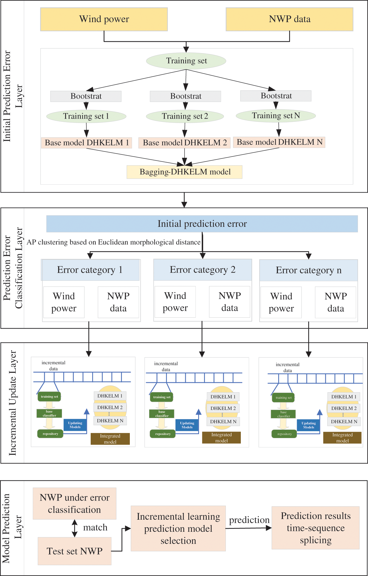
Figure 1: Full-text idea framework

3  Bagging-DHKELM Initial Wind Power Prediction Model

In this paper, the ensemble learning strategy is adopted as the framework for constructing the initial model, that mainly combines multiple base models into an ensemble model. Since individual learners may have their own defects, multiple models can comprehensively integrate the performance of multiple learners and have more comprehensive and robust performance. Different application scenarios can offer solutions using various combination strategies, and most ensemble models can solve problems that cannot be solved by individual learners.

Typically, the establishment of set model requires two stages, including basic model generation and set. There are significant differences in performance between different methods used to combine integrated models.

In the selection of base models, the DHKELM network among deep learning networks is selected as the basic model. Kernel Extreme Learning Machine (KELM) is a single hidden layer feedforward neural network based on kernel function. As the weights and deviations of hidden layers are randomly generated in extreme learning machines, the output may have collinearity problems. This leads to the decrease of algorithm accuracy. The introduction of kernel function can effectively overcome this randomness [19]. The kernel function plays an important role affecting the performance of KELM. A single kernel function is difficult to fully learn wind power historical data with nonlinear characteristics. Using different kernel functions is an effective way to improve the performance of prediction models. Considering that wavelet kernel function has good nonlinear ability, and RBF kernel function is a typical global function, this paper jointly constructs a mixed kernel function by combining wavelet kernel function and RBF kernel function. The wavelet kernel function expression is as follows:

kwt(xi,xj)=∏i=1ncos[p3(xi−xj)p2exp⁡(xi−xj22p12)](1)

where, kwt(xi,xj)—wavelet kernel function, which has good non-linear ability; p1, p2 and p3—wavelet kernel parameters.

The RBF kernel function expression is:

kRBF(xi,xj)=exp⁡(xi−xj2γ2)(2)

where, kRBF(xi,xj) —RBF kernel function, which has strong global characteristics; γ—kernel parameter of RBF. After weighted summation, the hybrid kernel function is shown in Eq. (3).

kD(xi,xj)=α⋅kwt(xi,xj)+(1−α)⋅kRBF(xi,xj)(3)

where, α—weight coefficient of the mixed kernel function. After introducing kD(xi,xj) kernel function, the kernel mapping is used to replace the random mapping, and the actual output of HKELM is:

{f(x)=h(x)HT(HHT+I/M)−1Y[KD(x,xj)⋮KD(x,xn)](ΩELM+I/M)−1Y(4)

{ΩEL.M=HHTΩ(i,j)=h(xi)h(xj)=k(xi,xj)(5)

where, ΩELM represents kernel matrix; M represents regularization coefficient; Y represents target matrix; I represents identity matrix.

In terms of learning ability and generalization ability, deep learning has strong advantages. Apply the idea of automatic encoder (AE) to ELM to form an ELM-AE structure, which is similar to an approximator and used to make the input and output of the network the same [20]. Multiple ELM-AE stacks form a deep learning network, and then the hybrid kernel mapping is used to replace the random mapping to form DHKELM. Compared to traditional deep learning algorithms, DHKELM adopts hierarchical unsupervised training, which can greatly reduce reconstruction error and achieve similarity between model input and output data. Its model is shown in Fig. 2.

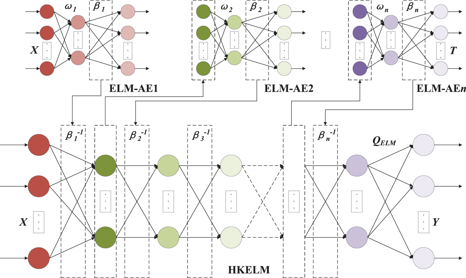
Figure 2: Network structure diagram of DHKELM

During the training process of the DHKELM network, the input data X is first sent to ELM-AE1 for training, and the output weight β1 is processed and sent to the underlying HKELM. The output matrix of the first hidden layer is used as the input of the second ELM-AE2, and after training, the output weight β2 is obtained. The system is sent to the underlying HKELM after processing, and several ELM-AEs are trained in turn. Finally, multiple cores are used for weighting to form a ΩELM kernel matrix, which replaces the random matrix HHT to obtain the output of DHKELM [21].

In the selection of integration method of integration model, considering the high demand of wind power data environment for model response speed, parallel direct integration method and integrates multiple basic models by Bagging-DHKELM algorithm are selected. Parallel integration method can effectively shorten the overall training time of model establishment. Moreover, it can be more efficient when the integrated model is dynamically updated and reconstructed. Fig. 3 is a schematic diagram of the Bagging-DHKELM Initial Wind Power Prediction Model.

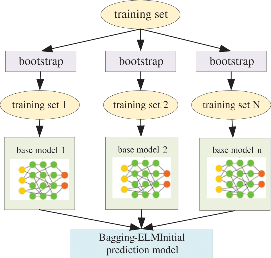
Figure 3: Bagging-DHKELM initial wind power prediction model

Based on the above Bagging-DHKELM initial wind power prediction model, the wind power data is trained and predicted to obtain the wind power prediction results for the second year, and the wind power prediction error for the second year is obtained based on the actual power and predicted power.

4  Cluster Analysis of Power Prediction Errors

This paper employs Affinity Propagation (AP) clustering method based on Euclidean morphological distance for clustering analysis of prediction error results. The AP clustering algorithm believes that all samples have the potential to become cluster centers. It selects a set of high-quality samples as cluster centers through “election” [22]. Compared to traditional clustering algorithms, the AP clustering algorithm can automatically determine the number of clusters and has higher stability [23,24]. On this basis, this article introduces Euclidean morphological distance to measure the similarity of error curves, further improving the clustering effect.

Firstly, concerning the determination of the number of error clusters, this paper opts for the count of clusters that corresponds to the superior clustering quality as the definitive quantity of error clusters. In terms of evaluating clustering quality, we select the DB index from the internal evaluation index and the modified index based on Euclidean morphological distance. The specific formula is as follows:

1)   DB indicator.

DB index can comprehensively consider the degree of agglomeration within clusters and the degree of separation between clusters, and its calculation formula is as follows:

IDB=1K∑k=1KRk(6)

Rk=maxk≠jd(Xk)+d(Xj)d(Ck,Cj)(7)

where, d(Xk) and d(Xj) are the average Euclidean distance between the sample points and the sample center in cluster Ck and cluster Cj, respectively, indicating the degree of aggregation between samples within a cluster; d(Ck,Cj) is the average Euclidean distance between the sample centers in cluster Ck and cluster Cj, indicating the degree of separation between two different clusters.

2)   Modified DB (MDB) index based on Euclidean morphological distance.

IMDB=1K∑k=1Kmaxk≠jdemd(Xk)+demd(Xj)demd(Ck,Cj)(8)

Both IDB and IMDB calculate the ratio of within-cluster similarity and between-cluster dissimilarity between any two clusters, so the lower the value, the higher the clustering quality. When selecting the optimal number of clusters, it is generally necessary to find its minimum point.

Secondly, in the implementation process of AP clustering algorithm, the similarity matrix S composed of the distance between pairs of samples is used as the input. The matrix element s(i,j) is generally a negative value of the Euclidean distance between sequences X and Y. The larger s(i,j), the more similar sequences X and Y. In this paper, the negative value of the Euclidean morphological trend distance is taken, as shown in Eq. (9).

s(i,j)=−Demd(X,Y)(9)

In addition to configuring similarity measurement schemes, the AP clustering scheme also controls the clustering effect of the algorithm by referring to the degree of reference p and damping coefficient λ. The reference degree is the diagonal element s(i,j) of the similarity matrix. In the algorithm, the final clustering result can be controlled by adjusting the reference degree. The larger the reference degree, the smaller the number of clusters. In order to avoid parameter oscillations during the clustering process, the default value of λ is set to 0.9 in this article.

5  Incremental Learning of Wind Power Prediction Model

After clustering the errors, corresponding NWP data labels are given according to the error categories, and different types of NWP data and their corresponding actual wind power prediction data are used as increments to update the initial model.

When a new incremental set Di is input, the base model of the integrated DHKELM model is continuously updated to ensure the stability of the integrated model. Integrated incremental learning usually requires a forgetting mechanism to remove the base model from the integrated model and add new base models to adapt to new data. In order to avoid catastrophic forgetting of knowledge, this paper dynamically reconstructs the integrated model Ei and uses eMAPE and R2 as indicators to achieve the optimization of the weight of the base learner integration. The optimization is solved using MPA, thus obtaining the optimal integration weight strategy between the base learners and the final prediction result. The method proposed in this article makes full use of the performance differences and complementary capabilities between the base learners. When facing different data sets, it can obtain the optimal integrated strong learner model through simple optimization, which has better performance than traditional average integration methods. The base learner integration weight optimization model based on eMAPE and R2 can be written as

{minJ=eMAPE(w1,w2,…,wm)+(1−R2(w1,w2,…,wm))s.t.∑i=1mwi=1eMAPE(w1,w2,…,wm)=1T∑t=1T|(w1lRVM1,t+w2lRVM2,t+…+wnlRVMm,t)−lreal,tlreal,t|∗100%R2(w1,w2,…,wm)=1−∑t=1T((w1lRVM1,t+w2lRVM2,t+…+wnlRVMm,t)−lreal,t)2∑t=1T(lmean,t−lreal,t)2}(10)

where, eMAPE and R2 represent the average absolute percentage error and coefficient of determination of the integrated prediction, respectively. The smaller eMAPE and the larger R2 indicate better wind power prediction performance. Both eMAPE and R2 have a value range of [0, 1]; w1,…,wn represent the integration weights of DHKELM1,t…DHKELMM,t, respectively. T is the number of samples. lDHKELM1,t, lDHKELM2,t,…,lDHKELMM,t represent the predicted values of each base learner for the t-th sample. lreal,t is the true value of the t-th wind power sample, and lmean,t is the average value of wind power samples.

For the newly input incremental sample set Di, eMAPE and R2 consider the accuracy of each DHKELM’s mapping learning for each sample, making the prediction results more objective and accurate. Additionally, the weight of each DHKELM in the integrated model Ei can be used to measure its importance in integrated decision-making. The performance of individual base models in the integrated model is measured using the results of integrated output. The DHKELM with the largest eMAPE and the smallest R2 value is considered to be the worst-performing base model for the new incremental set. This allows better performance evaluation of individual DHKELMs in the integrated model and enables identification and deletion of the worst-performing DHKELM during dynamic incremental updates. In each incremental step, the entire new incremental set is used as a validation set for dynamic ensemble reconstruction. As shown in Fig. 4, whenever a new input incremental set is input, the worst-performing DHKELMr is identified by calculating eMAPE and R2 values, and it is deleted when eMAPE > 0.03 and R2 < 0.95. At the same time, a new DHKELMDi is trained on the incremental set to replace it. By dynamically reconstructing the integrated model using eMAPE and R2 values for each integrated component DHKELM on the new incremental set, model obsolescence can be effectively avoided. Fig. 4 illustrates a schematic diagram of implementing incremental updates for models under a class by taking a type of NWP and corresponding actual wind power data as input.

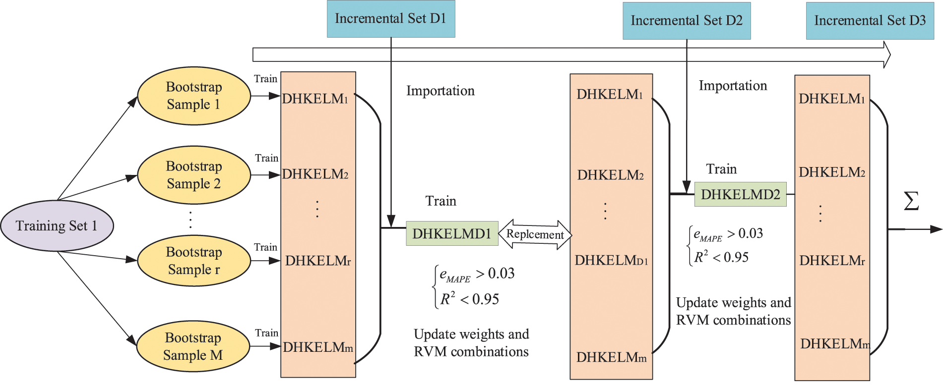
Figure 4: Schematic diagram of dynamic incremental learning of model

The evaluation indicators for prediction error are the standard root mean square error (INRMSE) and the standard mean absolute error (INMAE), namely

{INRMSE=∑k=1N(pk−pk,pre)2CapN×100%INMAE=∑k=1N|pk−pk,pre|CapN×100%∣(11)

where, pk and pk, pre are the measured and predicted values of wind power at time k, respectively; Cap is the installed capacity of the wind farm; N is the sample size of the prediction segment. The monthly standard root mean square error is taken as the evaluation criterion for improving prediction accuracy.

6  Experimental Results and Analysis

The hardware platform configuration of this paper is as follows: The processor is an i9-14900HX, the memory is 32 GB, the solid-state disk capacity is 1 TB, and the GPU graphics card is an RTX4060. The simulation software uses Python to build a deep neural network, with Keras as the front end and TensorFlow as the back end to write a software framework. A calculus analysis was conducted on 10 wind farms in a province in northeastern China, with a total installed capacity of 752.3 MW. The actual and predicted power for the entire year of 2021 were used as the data samples for the initial model, while the actual and predicted power from January to November of 2022 was used as the data samples for incremental model updates. The actual and predicted power for December 2022 were used as the test set, with a time resolution of 15 min and a prediction time scale of 1 day before, that is, the power from 0–24 h of the next day was predicted in the morning of each day.

6.1 Determination of the Number of Error Clusters

Using the AP clustering algorithm with Euclidean morphological distance, a clustering test was conducted on the error curve. The weight coefficients a and β for the two similarity measurement schemes were calculated using the entropy weight method, and were taken to be 0.6832 and 0.5275, respectively. The damping coefficient was set to 0.95, and the corresponding number of clusters was obtained by adjusting the reference degree p. The optimal number of clusters was selected using the DB index and MDB index. Fig. 5 shows the relationship between the number of clusters and clustering indicators.

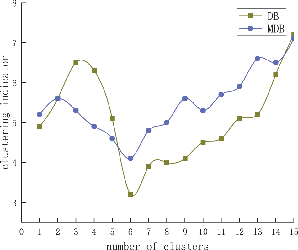
Figure 5: Relationship between the number of clusters and the clustering validity index

As shown in Fig. 5, when K = 6, both the DB and MDB metrics have the minimum value, so the errors are clustered into six categories. Fig. 6 shows the effect of error clustering.

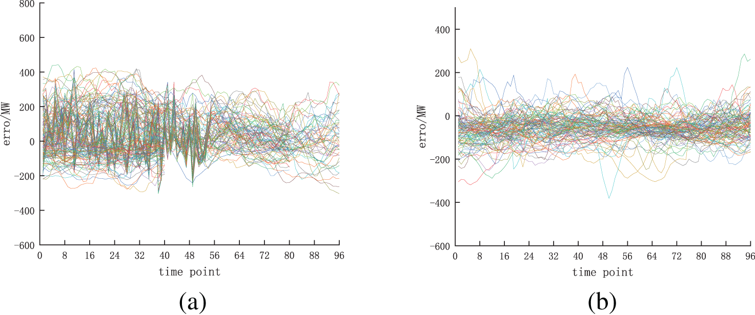
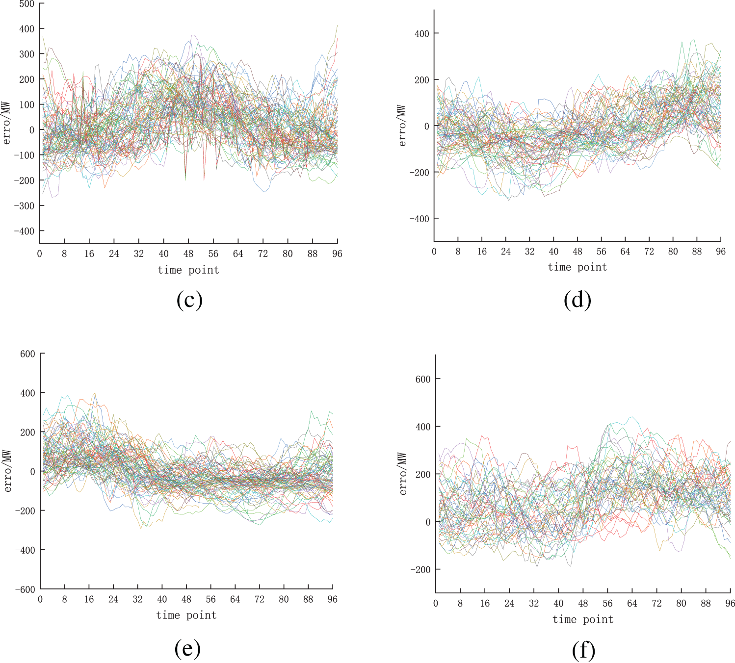
Figure 6: Error clustering effect

From the results shown in Fig. 6, it can be seen that the error in category c is relatively large, and the error in category f has a large fluctuation. By performing correlation analysis on NWP data under different error categories, it can be concluded that the average wind speed in NWP under categories c and f is the largest. This also proves that determining NWP data categories based on error classification is analyzable.

6.2 Analysis of Short-Term Wind Power Prediction Results

Mark NWP data under the above classification errors, and add the actual power and NWP data corresponding to each error as increments to the initial model for updating. Therefore, six types of incremental updating prediction models are produced. In addition, the test set NWP data is matched with the optimal prediction model based on correlation, and obtain the prediction results as shown in Fig. 7 and Table 1.

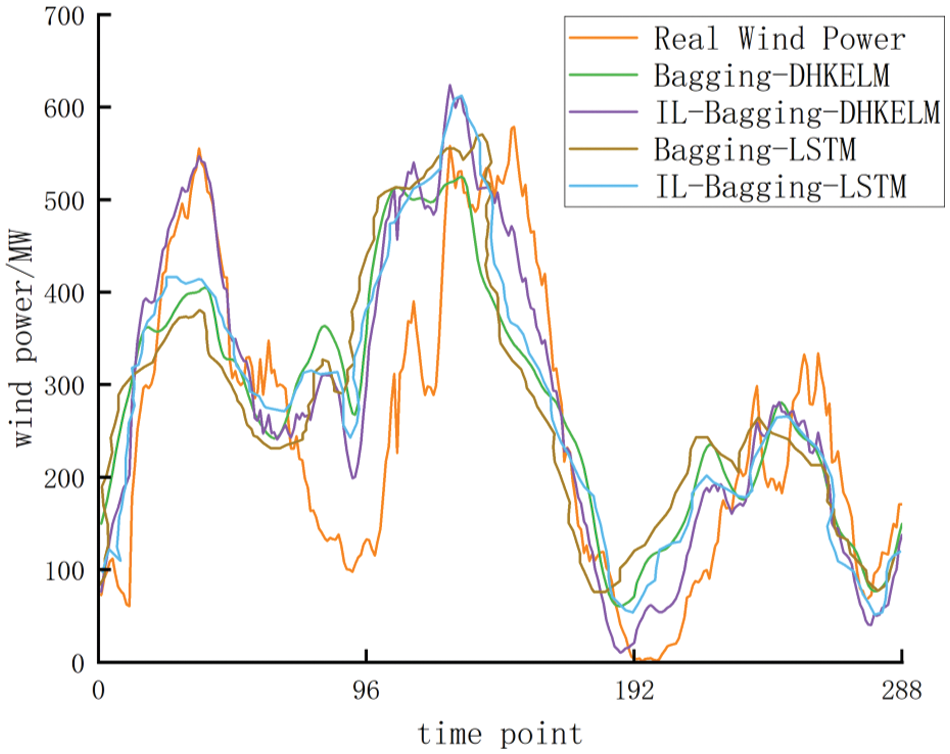
Figure 7: Results of wind forecasting curve

It can be seen from the prediction curve that using DHKELM as the basic model has better prediction performance than using LSTM as the basic model. Incremental learning is introduced into the initial set prediction model to improve the prediction accuracy. This can better track the wind power curve during the peak wind power period. Furthermore, it can be seen from the error index that compared with the initial model, INMSE and INRMSE of the incremental updating model based on integrated learning strategy have increased by 1.9 percentage points and 2.1 percentage points, respectively. Based on the above analysis, it can be concluded that the prediction model can effectively improve the accuracy of wind power forecasting.

7  Conclusion

An IL-Bagging-DHKELM short-term wind power prediction model based on error AP clustering analysis is proposed. An IL-Bagging-DHKELM short-term wind power forecasting model based on error AP clustering analysis is proposed. That model is suitable for current wind power, and it has the characteristics of strong randomness and large amount of data. The following conclusions can be drawn:

1)   AP clustering of input meteorological data using error features can deeply explore the influence of meteorological data on the accuracy of wind power prediction and effectively improve the accuracy of wind power prediction.

2)   In comparison with deep learning or ensemble learning, DHKELM model has more reliable prediction performance. Through the DHKELM model as the basic model and Bagging as the ensemble strategy framework, an effective combination of deep learning and ensemble learning strategies can be achieved.

3)   Wind power data and NWP data are used as incremental updates of Bagging DHKELM model, which effectively solves the problem of data redundancy. More importantly, the model parameters are updated, which effectively improves the generalization ability and prediction efficiency of the model.

Acknowledgement: Authors thank those who contributed to write this article and give some valuable comments.

Funding Statement: This work was funded by Liaoning Provincial Department of Science and Technology (2023JH2/101600058).

Author Contributions: Study conception and design: Jing Gao, Hongjiang Wang, Mingxuan Ji; data collection: Jing Gao, Mingxuan Ji; analysis and interpretation of results: Jing Gao, Mingxuan Ji; draft manuscript preparation: Jing Gao, Mingxuan Ji, Zhongxiao Du. All authors reviewed the results and approved the final version of the manuscript.

Availability of Data and Materials: If readers need data, they can contact my email: 1822682156@qq.com.

Conflicts of Interest: The authors declare that they have no conflicts of interest to report regarding the present study.

References

1. R. McKenna et al., “High-resolution large-scale onshore wind energy assessments: A review of potential definitions, methodologies and future research needs,” Renew. Energy, vol. 182, no. 10, pp. 659–684, Jan. 2022. doi: 10.1016/j.renene.2021.10.027. [Google Scholar] [CrossRef]

2. Z. Zhou, N. Zhang, X. Xie, and H. Li, “Key technologies and developing challenges of power system with high proportion of renewable energy,” Autom. Electr. Power Syst., vol. 45, no. 9, pp. 171–191, May 2021. doi: 10.7500/AEPS20200922001. [Google Scholar] [CrossRef]

3. S. M. Lin, S. Wang, X. F. Xu, R. X. Li, and P. M. Shi, “An adaptive spatiotemporal feature fusion transformer utilizing GAT and optimizable graph matrixes for offshore wind speed prediction,” Energy, vol. 292, no. 10, pp. 130404, Apr. 2024. doi: 10.1016/j.energy.2024.130404. [Google Scholar] [CrossRef]

4. X. F. Xu, S. T. Hu, P. M. Shi, H. S. Shao, R. X. Li and Z. Li, “Natural phase space reconstruction-based broad learning system for short-term wind speed prediction: Case studies of an offshore wind farm,” Energy, vol. 262, no. 11, pp. 125342, 2023. doi: 10.1016/j.energy.2022.125342. [Google Scholar] [CrossRef]

5. N. Li, L. B. Ma, G. Yu, B. Xue, M. J. Zhang and Y. C. Jin, “Survey on evolutionary deep learning: Principles, algorithms, applications and open issues,” ACM Comput. Surv., vol. 56, no. 2, pp. 1–34, Sep. 2023. doi: 10.48550/arXiv.2208.10658. [Google Scholar] [CrossRef]

6. Y. L. Zhou, G. Z. Yu, J. F. Liu, Z. H. Song, and P. Kong, “Offshore wind power prediction based on improved long-term recurrent convolutional neural network,” Autom. Elect. Power Syst., vol. 45, no. 3, pp. 183–191, Mar. 2021. doi: 10.7500/AEPS20191212003. [Google Scholar] [CrossRef]

7. Y. F. Chang, Z. X. Yang, F. Pan, Y. Tang, and W. C. Huang, “Ultra-short-term wind power prediction based on CEEMDAN-PE-WPD and multi-objective optimization,” Power Syst. Technol., vol. 47, no. 12, pp. 5015–5026, Dec. 2023. doi: 10.13335/j.1000-3673.pst.2022.1367. [Google Scholar] [CrossRef]

8. M. Li, M. Yang, Y. Yu, P. Li, and Q. Wu, “Short-term wind power forecast based on continuous conditional random field,” IEEE Trans. Power Syst., vol. 39, no. 1, pp. 2185–2197, Jan. 2024. doi: 10.1109/TPWRS.2023.3270662. [Google Scholar] [CrossRef]

9. X. M. Ma and D. Xu, “Incremental learning for robots: A survey,” Control and Decision, vol. 39, no. 5, pp. 1409–1423, 2023. doi: 10.13195/j.kzyjc.2023.0631. [Google Scholar] [CrossRef]

10. L. Ma et al., “Pareto-wise ranking classifier for multi-objective evolutionary neural architecture search,” in IEEE Transactions on Evolutionary Computation, Sep. 2023. doi: 10.1109/TEVC.2023.3314766. [Google Scholar] [CrossRef]

11. Z. Tian, C. Shen, H. Chen, and T. He, “FCOS: Fully convolutional one-stage object detection,” in 2019 IEEE/CVF Int. Conf. Comput. Vis. (ICCV), Seoul, Korea (South2019, pp. 9626–9635. doi: 10.1109/ICCV.2019.00972. [Google Scholar] [CrossRef]

12. S. Ren, K. He, R. Girshick, and J. Sun, “Faster R-CNN: Towards real-time object detection with region proposal networks,” IEEE Trans. Pattern Anal. Mach. Intell., vol. 39, no. 6, pp. 1137–1149, Jun. 2017. doi: 10.1109/TPAMI.2016.2577031. [Google Scholar] [PubMed] [CrossRef]

13. L. Ma, H. Kang, G. Yu, Q. Li, and Q. He, “Single-domain generalized predictor for neural architecture search system,” IEEE Trans. Comput., vol. 73, no. 5, pp. 1400–1413, May 2024. doi: 10.1109/TC.2024.3365949. [Google Scholar] [CrossRef]

14. C. Y. Pan, W. L. Wen, M. Zhu, C. C. Hou, J. J. Ma and X. P. Kong, “Online ultra-short-term wind power forecasting based on concept drift detection and incremental updating mechanism,” (in ChineseProc. CSEE. Accessed: Feb. 19, 2024. [Online]. Available: https://link.cnki.net/urlid/11.2107.TM.20231227.0928.002 [Google Scholar]

15. L. Ye, B. H. Dai, Z. Li, M. Pei, Y. N. Zhao and P. Lu, “An ensemble method for short-term wind power prediction considering error correction strategy,” Appl. Energy, vol. 322, no. 1, pp. 119475, Sep. 2022. doi: 10.1016/j.apenergy.2022.119475. [Google Scholar] [CrossRef]

16. J. F. Song et al., “Short-term wind power prediction based on deviation compensation TCN-LSTM and step transfer strategy,” Southern Power Syst. Technol., vol. 17, no. 12, pp. 71–79, Dec. 2024. doi: 10.13648/j.cnki.issn1674-0629.2023.12.009. [Google Scholar] [CrossRef]

17. C. Li, G. Tang, X. Xue, A. Saeed, and X. Hu, “Short-term wind speed interval prediction based on ensemble GRU model,” IEEE Trans. Sustain. Energy, vol. 11, no. 3, pp. 1370–1380, Jul. 2020. doi: 10.1109/TSTE.2019.2926147. [Google Scholar] [CrossRef]

18. L. B. Ma, X. Y. Wang, X. W. Wang, L. Wang, L. Shi and M. Huang, “TCDA: Truthful combinatorial double auctions for mobile edge computing in industrial internet of things,” IEEE Trans. Mob. Comput., vol. 21, no. 11, pp. 4125–4138, Nov. 2022. doi: 10.1109/TMC.2021.3064314. [Google Scholar] [CrossRef]

19. C. S. Zhu and K. P. Zhao, “Wind power prediction of kernel extreme learning machine based on improved grey wolf algorithm,” Comput. Appl. Softw., vol. 39, no. 5, pp. 291–298, May 2022. doi: 10.3969/j.issn.1000-386x.2022.05.044. [Google Scholar] [CrossRef]

20. F. H. Li and Y. Q. Xiao, “Short-term power load forecasting based on EMD-TCN-ELM,” Comput. Syst. & Appl., vol. 31, no. 11, pp. 223–229, Nov. 2022. doi: 10.15888/j.cnki.csa.008781. [Google Scholar] [CrossRef]

21. L. Q. Shang, C. H. Huang, Y. D. Hou, H. B. Li, Z. Hui and J. T. Zhang, “Short-term wind power prediction by using the deep kernel extreme learning machine with well-selected and optimized features,” (in ChineseJ. Xi’an Jiaotong Univ., vol. 57, no. 1, pp. 66–77, Jan. 2023. doi: 10.7652/xjtuxb202301007. [Google Scholar] [CrossRef]

22. J. Q. Lai, “Research on adaptive AP clustering algorithm,” Comput. Era, no. 4, pp. 38–42, Apr. 2022. doi: 10.16644/j.cnki.cn33-1094/tp.2022.04.010. [Google Scholar] [CrossRef]

23. L. Ye et al., “Wind power time series aggregation approach based on affinity propagation clustering and MCMC algorithm,” (in ChineseProc. CSEE, vol. 40, no. 12, pp. 3745–3753, Jun. 2020. doi: 10.13334/j.0258-8013.pcsee.190788. [Google Scholar] [CrossRef]

24. Z. Z. Chu, J. Liang, X. Zhang, X. M. Dong, and Y. L. Zhang, “Modeling of generalized load steady-state characteristics based on affinity propagation clustering algorithm and its application,” Elect. Power Autom. Equip., vol. 36, no. 3, pp. 115–123, Mar. 2016. doi: 10.16081/j.issn.1006-6047.2016.03.018. [Google Scholar] [CrossRef]