Enhancing Hyper-Spectral Image Classification with Reinforcement Learning and Advanced Multi-Objective Binary Grey Wolf Optimization

1  Introduction

The classification of hyperspectral (HS) images stands as a vital process in extracting meaningful information from the vast and complex data these images provide [1]. HS imaging gathers data over a broad portion of the electromagnetic spectrum, extending well past the visual capabilities of the human eye, and records the distinctive spectral fingerprint of every pixel [2]. The classification task involves assigning each pixel to a specific class based on its spectral signature, effectively differentiating between various materials or objects within the scene. The use of HS image classification, coupled with the ever-growing computational power and advanced analytical techniques, presents a paradigm shift in how we observe and interpret the world around us. It allows for an unprecedented level of detail in analysis, which, in turn, translates into better decision-making across a spectrum of applications, from managing natural resources to enhancing various communication infrastructure security [3–6].

This technique is particularly potent due to its fine spectral resolution, which allows for the discrimination between objects that would appear identical in traditional RGB imagery. For instance, in precision agriculture, this granularity enables farmers to distinguish between plant species and their respective health statuses, allowing for targeted interventions that can optimize yield and reduce waste [7]. HS image classification in urban areas serves as a transformative tool for urban management by providing a detailed spectral understanding of the cityscape. This detailed view is essential for urban planners, policymakers, and environmentalists who strive to enhance the livability, sustainability, and resilience of urban environments. In the urban context, the ability to classify the different elements of an urban landscape allows for efficient land-use planning. Urban sprawl can be monitored, and the encroachment of built-up areas on natural environments can be tracked with precision [8].

Multispectral (MS) and HS imaging are key techniques in agriculture for crop monitoring, disease detection, and yield estimation, capturing data at multiple wavelengths [3]. MS imaging uses fewer spectral bands (3–10) covering broader wavelength ranges, making data processing easier and faster, suitable for real-time applications with limited resources. In contrast, HS imaging uses hundreds of narrower bands, providing finer spectral resolution and more detailed spectral signatures, but requires more complex data processing due to larger data volumes. While HS offers more precise and accurate analysis, MS is still accurate enough for many applications and offers advantages in cost, simplicity, and speed. The choice between MS and HS imaging depends on the application’s specific needs for detail, accuracy, and operational constraints [7].

The classification of HS images inherently deals with the intricate task of sifting through an abundance of data contained within numerous spectral bands. Each band represents a narrow wavelength interval of the electromagnetic spectrum and potentially holds crucial information about the material properties within the imaged scene. However, not all bands contribute meaningful data for classification purposes; some may carry redundant information or noise that can convolute the analysis and lead to less accurate outcomes [9–11]. In scenarios where the primary goal is to classify objects or materials within an image, the effectiveness of classifiers is highly contingent upon the quality and the dimensionality of the feature space. A feature space bloated with a high number of spectral bands can overwhelm classifiers, leading to the Hughes phenomenon. This phenomenon highlights a paradox in pattern recognition: With an increase in dimensionality, the classifier’s performance can degrade unless there is a proportionate increase in the training samples. The reason for this degradation is that with more dimensions, the volume of the feature space increases exponentially, and the available training samples become sparse, making it difficult for the classifier to generalize from the training data to new, unseen data [12–14].

Moreover, the presence of redundant bands in HS images can have several detrimental effects on the classification process. It can exponentially increase the computational burden, as the algorithms have to process a larger volume of data. This not only slows down the analysis but also requires more computational resources, which may not be feasible in all application scenarios [15–17]. Moreover, the existence of noise and closely linked bands may conceal the actual signal, complicating the task of classifiers in precisely differentiating between various classes. This can result in lower precision and recall rates in classification tasks, reducing the overall reliability of the analysis.

The act of band selection or dimensionality reduction, therefore, becomes a pivotal step in the preprocessing of HS data. By employing feature selection techniques, researchers aim to extract the most informative and discriminative bands for the task at hand [9–12]. This process not only simplifies the classifier’s model by reducing the complexity of the feature space but also enhances the classifier’s ability to make accurate predictions by focusing on the most relevant information. Additionally, the removal of redundant bands leads to faster processing times and less demanding storage requirements, facilitating more efficient and scalable applications of HS imaging in diverse fields [17–19].

1.1 Related Works

The utilization of meta-heuristic algorithms like the gray wolf optimizer (GWO) in the selection of optimal bands for HS images is a response to the inherent complexity and high dimensionality of HS data [5,9–12]. HS images can contain hundreds of bands, and not all of these bands are equally useful for classification tasks. Some bands may contain redundant information, while others may contain noise that obscures the meaningful data. Meta-heuristic algorithms, which are inspired by natural processes and behaviors, provide a way to navigate the vast search space efficiently and effectively [20–23]. GWO imitates the social structure and predatory strategies of gray wolves in nature. GWO is especially valuable because it balances exploration and exploitation: It explores the search space to avoid local minima and exploits the best solutions to converge upon an optimal set of bands [24–26]. By doing so, it eliminates unnecessary bands, thereby reducing computational load, improving classification accuracy, and enhancing the overall efficiency of the HS image processing [17–19].

Reinforcement learning (RL), such as deep Q-learning (DQL), offers a different approach to HS image classification [27–31]. The classification of HS images through DQL represents a significant leap in the analytical capabilities of remote sensing (RS). HS images, with their high-dimensional spectral information, pose a unique challenge. Traditional methods can become overwhelmed by the sheer volume and complexity of the data, leading to inefficiencies or inaccuracies in classification [32]. DQL, a sophisticated machine learning (ML) technique, brings a dynamic approach to tackling this challenge, fundamentally altering the way we process and interpret HS data. DQL distinguishes itself by learning to make decisions. It does this by interacting with the environment and learning from the outcomes of its actions [33]. In an HS image, each pixel can be considered an agent that needs to be classified based on its spectral signature. DQL navigates through this multidimensional space and incrementally improves its classification decisions through trial and error, guided by a reward system. This system penalizes the algorithm for incorrect classifications and rewards it for correct ones, leading to a continuous refinement of the decision-making policy. What makes DQL particularly well-suited to HS image classification is its ability to handle the complexity and subtlety of the data. HS images are not just large; they contain subtle spectral differences that can be crucial for accurate classification. The depth of layers in a deep learning (DL) model [34–38] allows for the extraction of high-level features from raw spectral data, which is essential when dealing with fine-grained differences between classes [39–41]. Moreover, DQL does not require pre-labeled data to the same extent as supervised learning algorithms, which is a significant advantage when such labels are scarce or expensive to obtain.

The combination of DQL with meta-heuristic methods like GWO can be particularly potent for HS image classification. Meta-heuristic approaches can be used to diminish the complexity of the feature space by choosing the most suitable bands. The reduced, more relevant feature space can then be processed using DQL, which benefits from the cleaner, more focused data to improve its classification performance. This synergistic approach leverages the strengths of both methods: The global search capabilities of GWO for feature selection and the adaptive, learning-based nature of DQL for classification. By integrating these two approaches, the combined method can handle the vast data volumes and complexity of HS images more effectively than either approach could alone. It allows for the processing of HS data in a way that is both computationally efficient and highly accurate, making it well-suited for real-world applications where speed and precision are of the essence.

In numerous studies, researchers have employed meta-heuristic algorithms to identify the most effective spectral bands, while machine learning architectures have been utilized to categorize HS images [5,42–45]. Ghadi et al. [5] developed an innovative migration-based particle swarm optimization (MBPSO) tailored for the optimal selection of spectral bands. They utilized the variance-based J1 criteria as a fitness function in MBPSO and leveraged a support vector machine (SVM) for classification purposes. The efficacy of their proposed method was tested across four different HS datasets. The findings indicated that their MBPSO algorithm outperformed competing algorithms in terms of numerical performance, achieving higher accuracy with a reduced set of features.

Reddy et al. [17] developed a compressed synergic deep convolution neural network enhanced with Aquila optimization (CSDCNN-AO) for HS image classification, which incorporates a novel optimization technique known as AO. Their experimental evaluation encompassed four datasets. Testing across these four HS datasets revealed that this innovative approach surpassed traditional methods in standard evaluation metrics, including average accuracy (AA), overall accuracy (OA), and Kappa coefficient (KC). Furthermore, this technique significantly shortened the training time and reduced computational requirements, resulting in enhanced training stability, optimal performance, and outstanding training accuracy. Dhingra et al. [18] explored a range of meta-heuristic strategies combined with neural networks for classifying HS images, frequently employing the cuckoo search (CS) optimization algorithm. They enhanced the capability of CS by incorporating the fitness function from the genetic algorithm (GA). This hybrid CS-GA algorithm was responsible for feature selection, and the selected features were subsequently used to train and classify using an artificial neural network (ANN). Their algorithms were evaluated on the Indian Pines dataset. The innovative approach of combining CS and GA with ANN surpassed two previously established methods, achieving an OA of 97.30% and KC of 97.60%.

Sawant et al. [19] introduced an innovative band selection method using a novel meta-heuristic to address the challenge of the curse of dimensionality. They developed a modified wind-driven optimization (MWDO) technique for band selection, designed to prevent premature convergence and balance the exploration-exploitation trade-off in searching. To enhance classification performance further, the selected bands were incorporated into a DL model for extracting high-level, useful features. The results demonstrated that their approach effectively chose an optimal subset of bands, achieving superior classification accuracy with fewer bands compared to other methods. Their suggested approach achieved OA of 93.26%, 94.76%, and 95.96% for the Indian Pines, Pavia University, and Salinas datasets, respectively.

Wang et al. in their study [42] presented a technique termed region-aware hierarchical latent feature representation. This technique involves initially segmenting HS images into various regions using a superpixel segmentation algorithm, ensuring the preservation of spatial data. The procedure concludes by implementing k-means clustering on a unified feature representation matrix, leading to the creation of multiple clusters. From there, the band with the greatest information entropy is selected to form the final band subset. Extensive experimental findings indicate that this clustering method surpasses existing top techniques in selecting bands. Tang et al. [43] introduced a self-representation model for selecting bands in HS images without relying on labeled data, briefly named S4P. This technique stands out from previous methods because it does not convert each band into a feature vector. Rather, it employs the first principal component of the original HS cube, segmented into multiple superpixels, to capture the spatial configuration of homogeneous areas. To validate the efficacy of S4P, comprehensive experiments and analyses were carried out on three public datasets, demonstrating its enhanced performance over other prominent methods in the discipline.

In the aforementioned studies, the significance of employing meta-heuristic algorithms and ML architectures is consistently emphasized. Consequently, in our paper, we have adopted a novel approach by utilizing a multi-objective binary gray wolf optimizer deep Q-learning (MOBGWO-DQL) for the selection of optimal spectral bands. To validate the efficacy of our methodology, we conducted experiments on widely recognized HS image datasets, specifically the Pavia University and Indian Pines datasets. Our findings will be benchmarked against traditional DL models and other meta-heuristic methods to ascertain the relative performance and effectiveness of the proposed MOBGWO-DQL framework.

1.2 Paper Contributions

•   This paper investigates a novel MOBGWO for optimal band selection and uses a DQL model to further enhance the accuracy of HS image classification. The primary objective of this model is to reduce the number of bands while maximizing classification accuracy.

•   In the suggested MOBGWO, a new sigmoid function is introduced as a transfer function to modify the wolves’ position. The core advantage of MOBGWO lies in its adeptness at maintaining equilibrium between exploration and exploitation.

•   The performance of the proposed MOBGWO-DQL is compared against nine ML algorithms, namely standard MOGWO, multi-objective orchard algorithm (MOOA), multi-objective beluga whale optimization (MOBWO), MOGA, recurrent neural network (RNN), long short-term memory (LSTM), deep neural network (DNN), SVM, and random forest (RF).

•   To evaluate the proposed models, three well-known datasets, Pavia University, Washington Mall, and Indian Pines, are utilized. Furthermore, the analysis of the results employs several criteria, including class accuracy, OA, KC, receiver operating characteristic (ROC) curves, root mean square error (RMSE), and convergence curves. The results of the simulations show that the MOBGWO-DQL model outperforms other models in terms of performance.

1.3 Paper Organization

The layout of the paper is structured as follows: Section 2 provides an overview of the dataset and the MOBGWO-DQL model being proposed. Section 3 focuses on the comparative performance analysis of the suggested algorithm for HS image classification relative to nine different algorithms. Concluding remarks are offered in Section 4.

2  Research Method

Fig. 1 depicts the workflow of the research approach, which is segmented into four principal phases. The first phase is dedicated to preprocessing, involving the removal of noisy and water-absorption bands from the HS images. The next phase proceeds with implementing the proposed band selection technique on the previously prepared test and training samples. During this phase, various meta-heuristic algorithms are employed on these samples to evaluate their efficiency in identifying the optimal bands. The third phase capitalizes on the results from the band selection phase, where the optimal spectral bands selected for each dataset are utilized in both RL and DL classifiers. The workflow culminates in an exhaustive evaluation of the outcomes, providing a comprehensive analysis of the band selection methods and their impact on classification accuracy.

Figure 1: The block diagram of the research method

2.1 Standard GWO

GWO [21] is an algorithm inspired by the behavior and social structure of grey wolves. It is a meta-heuristic approach used for solving optimization challenges, replicating the way wolf packs interact and hunt. The algorithm employs a group of wolves, symbolizing possible solutions, to navigate complex optimization spaces. It incorporates the pack’s social order, with alpha (α), beta (β), delta (δ), and omega (ω) wolves, each playing a leadership role (Fig. 2). These leaders influence the exploration process, adjusting their strategies according to their own effectiveness and the movements of fellow wolves.

Figure 2: Gray wolf hierarchy

Within a wolf pack, leadership is typically assumed by an alpha male and female pair, who make key decisions about hunting, resting places, and daily activities. These alphas, while often leading, also show a level of democratic behavior by considering the input of other pack members. They alone have the right to mate within their group. Beta wolves, who are second in the hierarchy, support the alphas in their decision-making processes and can be of either gender. They are the likely successors to the alphas and must balance respect for them with authority over the lower-ranking wolves [21].

At the bottom of the social structure is the omega wolf, the most submissive and often the last to eat, obliged to follow the commands of those higher in rank. Omegas play a vital role in preserving the peace and stability of the pack, as their presence helps to mitigate conflicts and maintain the social order. Additionally, there are subordinate or delta wolves, assuming various roles such as scouts, guards, elders, hunters, and caretakers. They operate under the direction of the alphas and betas, while also exerting control over the omegas. These roles are critical for the overall functioning of the pack, encompassing duties like monitoring the territory’s borders, ensuring safety, and caring for the weak or injured members. GWO progresses through three primary stages in each cycle:

•   Initialization Stage: This involves randomly assigning initial positions to α, β, and δ wolves within the search area. These positions symbolize potential solutions to the problem at hand.

•   Search Phase: During this phase, the rest of the wolf pack adjusts their positions in relation to α, β, and δ wolves. This movement is guided by the pack’s social structure and the principles of exploration (searching new areas) and exploitation (focusing on promising areas). The algorithm is designed to find an equilibrium between these two strategies for efficient problem-solving.

•   Update Process: In this final stage, the positions of α, β, and δ wolves are revised according to their performance and the positions of other pack members. This step is crucial for improving the leaders’ positions, thereby steering the entire group towards more optimal solutions.

The mathematical framework of the GWO is outlined below. In this algorithm, the hunting process is led by α, β, and δ wolves, with ω wolves following the lead of these three groups. Reflecting the behavior observed in grey wolves, where they surround their prey during a hunt, a set of Eqs. (1)–(4) are introduced to mathematically model this encircling action [21]:

D→=C→X→p(t)−X→(t)(1)

X→(t+1)=C→X→p(t)−A→.D→(2)

A→=2a→r→1−a→(3)

C→=2r→2(4)

where X→p is hunting position vector, X→ is the position vector of a gray wolf, A→ and C→ are coefficient vectors, r→1 and r→2 are random vectors in the interval [0, 1], the a→ vector is linearly reduced from 2 to 0 during the repetition.

In modeling the hunting tactics of gray wolves mathematically, it is presupposed that α, together with the β and δ wolves, possess an enhanced knowledge of the prey’s potential location. Consequently, the algorithm preserves the three leading solutions identified and mandates that other searching agents, including ω wolves, adjust their positions in accordance with the top-performing agents. This strategy is captured in Eqs. (5)–(7), designed to support this facet of the simulation.

D→α=|C→1X→α−X→|,D→β=|C→2X→β−X→|,D→δ=|C→3X→δ−X→|(5)

X→1=X→α−A→1.(D→α)X→2=X→β−A→2.(D→β),X→3=X→δ−A→3.(D→δ)(6)

X→(t+1)=X→1+X→2+X→33(7)

Fig. 3 demonstrates how a search agent’s position is modified in 2D search space, guided by the positions of α, β, and δ wolves. Essentially, the new position of the search agent falls within a randomly chosen area inside a circle, the size of which is dictated by where α, β, and δ are located. Fundamentally, the alpha, beta, and delta wolves estimate the location of the prey, leading the other wolves to intermittently reposition themselves in the area around the prey [21].

Figure 3: Updating the position in the standard GWO

2.2 Proposed MOBGWO

The development of a new binary variant of the GWO is driven by the increasing demand for robust and versatile optimization algorithms across various scientific, engineering, and industrial domains. Originally modeled after the social hunting strategies of grey wolves, the conventional GWO has proven successful in addressing continuous optimization challenges. However, its application to problems involving discrete variables remains limited. This gap highlights the need to enhance the GWO framework, allowing it to effectively tackle discrete optimization issues through a bi-nary adaptation.

Moreover, optimization algorithms are crucial in managing multi-objective and high-dimensional problems, which are typically resource-intensive and time-consuming [46,47]. Consequently, there is a continuous effort among researchers and industry experts to refine existing methods or develop new strategies to boost optimization processes in terms of both efficiency and effectiveness. The introduction of a new MOBGWO is an endeavor to harness the algorithm’s potential for resolving discrete and multi-objective optimization tasks, thereby providing a robust instrument for a broader spectrum of practical implementations. In binary meta-heuristic algorithms [48] such as the BGWO, the transfer function is essential for shifting from a continuous to a discrete search space, where it deals with binary decision variables (0 and 1 s). This function is crucial as it facilitates the algorithm’s ability to toggle between binary states, adapting to situations where traditional algorithms are more geared towards continuous variables.

Acting as a pivotal decision-making entity, this function evaluates the probability of changing binary values, taking into account the algorithm’s present condition, the effectiveness of the solutions, and potential random factors. Its design is integral to the algorithm’s strategy in navigating the search space, striking a balance between uncovering new possibilities (exploration) and honing in on viable options (exploitation). In essence, it serves as a regulatory tool, guiding the algorithm in sifting through various potential solutions, with the aim of optimizing binary variables to enhance results while adeptly moving through the discrete search environment.

The development and refinement of this transfer function are key to crafting a successful binary meta-heuristic algorithm, as they play a significant role in its search performance and ability to converge effectively. Current research highlights the importance of sigmoid functions in developing these transfer functions. In line with this, our paper presents a novel application of sigmoid functions to tailor the GWO algorithm for binary optimization challenges. The innovative approach introduced in the MOBGWO centers around the development of a position update equation, detailed in Eq. (8). This is accomplished through the application of a novel sigmoid function, which serves as the transfer mechanism and is outlined in Eq. (9).

Xdt+1={1 if sigmoid(X1+X2+X33)≥R0otherwise(8)

Sigmoid(x)=11+γe−τ(x−μ)(9)

where Xdt+1 is the updated binary position; Sigmoid(x) is the novel transfer functions; μ is a random number ∈[0.37,0.63]; τ is a threshold number ∈(20,21,22,23); R is a random number ∈[0,1];γ is a random number ∈[0.93,1].

The aim of this paper is to identify the smallest set of optimal bands that yield the highest classification accuracy. In this context, a wolf represents an array of K features, as depicted in Fig. 4 (using binary coding). Within this array, each gene assigned a value of 1 signifies the inclusion of that band for classification purposes, whereas a gene with a value of zero indicates that the band is not chosen.

Figure 4: Definition of a wolf in the MOBGWO

In this paper, we employed two objective functions for HS image classification: Achieving the highest OA and minimizing the number of bands. To combine these objectives, we utilized the weighted sum method. Consequently, we defined the fitness function, which is presented as Eq. (10).

Fitness Function(j)=φ.OA(j)+(1−φ).log10⁡Kk(j)(10)

where OA(j) is the OA of the jth  wolf, K= number of bands, and k(j) is the number of bands selected in the jth  wolf. Moreover, the weight parameter φ is assigned a value of 0.89. This specific value for φ was determined through a process of trial and error. In order to identify the optimal setting for each parameter, all other variables were held constant while the objective function was tested with various parameter values.

2.3 DQL

RL is a method of ML that utilizes a trial-and-error approach. In this technique, an agent, which is the entity executing actions, responds to situations and in return, obtains a numerical reward. The agent’s objective is to optimize the accumulation of these reward points. A comprehensive discussion of RL is presented in references [31–33]. The fundamental elements of RL include:

•   The Environment: This pertains to the artificial physical environment in which the agent functions. It allows the agent to predict the rewards and outcomes of its actions prior to their execution.

•   The Agent: This is the key component in RL that engages in learning and action execution. The goal of an RL agent is to maximize the rewards it gains over time.

The Policy: This aspect dictates the possible actions (a) the agent may choose at any given moment. The policy (π) is elaborated in Eq. (11).

a=π(s)(11)

The Reward: The reward in RL is the score that an agent receives from the environment after taking an action. This value is indicative of the action’s effectiveness, serving as a gauge of its quality. In this context, the reward is essentially the environment’s reaction or feedback to the agent’s action. The agent uses this reward to comprehend the consequences of its actions and to formulate a model of the environment. This aspect is vital for the learning process. Particularly in the context of managing traffic signals to improve traffic flow, the reward is determined by different measures of traffic efficiency, including delay, waiting time, average speed, and the volume of vehicles passing through an intersection. This approach helps the agent to determine if a particular action (a) either diminishes or boosts the efficiency of an intersection. The reward Rsa, associated with a state s and an action a, is detailed in Eq. (12).

Rsa=E[Rt+1|st=s,At=a](12)

The State: The state in RL symbolizes the agent’s perception of the environment at each step. The value of the state denoted as V(s), is articulated in Eq. (13), where γ represents the discount factor, ranging between 0 and 1.

V(s)=E[Rt+1+γ.Rt+2+γ2.Rt+3|st=s](13)

Fig. 5 shows the interaction between an RL agent and the environment. RL algorithms can be broadly classified into three main types: Value-based, policy-based, and model-based algorithms. Each type has its own unique approach to learning and decision-making. Each of these algorithms has its strengths and weaknesses. Value-based methods excel in problems with a discrete and not too large action space. Policy-based approaches excel in environments with high-dimensional or continuous action spaces. On the other hand, model-based strategies can efficiently use fewer samples but depend on having an accurate model of the environment, which may be challenging to achieve in intricate settings. In this paper, the DQL algorithm is employed [31–33].

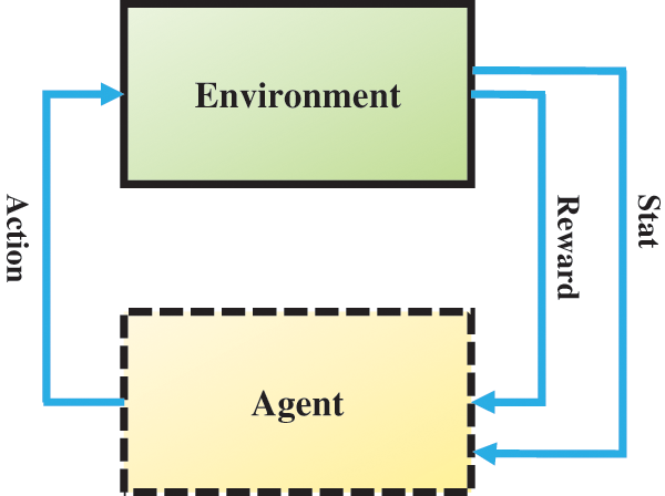
Figure 5: Schematic view of the RL tasks

Q-Learning is a type of RL that does not rely on a predefined model of the environment. It employs a trial-and-error method to navigate through environments that are both complex and unpredictable. The goal of Q-Learning is to develop a learning mechanism based on pairs of situations and actions, which are then evaluated through positive or negative rewards. In this approach, a distinct table is maintained to keep track of Q-values, which correspond to the states and actions of the agent. These Q-values are revised continuously throughout the learning process. The agent utilizes this table to select the most suitable action. DQL, which integrates RL and DL, employs DNNs as function approximators to identify the optimal Q-values for actions. The Q-values are determined using DL techniques [49,50].

2.4 Datasets

This paper utilizes three HS images, namely Indian Pine, Pavia University, and Washington Mall, which are commonly used as benchmark images in band selection studies. Table 1 displays the total number of samples for these HS images, along with the division into training and testing sets.

The first dataset in this study features HS images captured by AVIRIS sensor at the Indian Pines test site in northwest Indiana. This dataset is particularly notable for its detailed representation of a diverse landscape, primarily consisting of agricultural land and natural vegetation. Here is a more in-depth look at its characteristics:

•   Land composition: Over 60% of the area is agricultural, while the remaining 30% comprises forests and other types of natural vegetation. This varied landscape makes the dataset ideal for studies in land cover classification and agricultural monitoring.

•   Spectral bands and resolution: The image from this dataset has 220 spectral bands. This high number of bands is due to the sensor’s spectral resolution of 10 nanometers, allowing for a detailed spectral analysis across a wide range of wavelengths.

•   Wavelength coverage: The dataset encompasses the full range of electromagnetic waves from 400 to 2400 nanometers. This broad wavelength range includes both the visible and the near-infrared parts of the spectrum, providing comprehensive information about the surface characteristics.

•   Preprocessing and band removal: Due to factors like noise and water vapor absorption, certain spectral bands (specifically bands 1–3, 103, 109–112, 148–149, 164–165, 217–219, 104–108, 150–163, and 220) were identified as unreliable and subsequently removed from the analysis. This preprocessing step is crucial for enhancing the quality and reliability of the data.

•   Subset and pixel size: The specific subset used in this study consists of 145 ×145 pixels, each with a size of 20 meters. This resolution offers a balance between detailed surface information and manageable data size for analysis.

•   Classes and land cover types: The dataset is classified into 16 different categories, representing a mix of agricultural lands, forest areas, and urban regions. This classification provides a comprehensive understanding of the land cover types in the area, useful for applications in environmental monitoring, urban planning, and resource management.

Overall, the Indian Pines dataset, with its varied landscape, high spectral resolution, and comprehensive wavelength coverage, serves as a valuable resource for advanced RS research and applications, particularly in the fields of agriculture, forestry, and land cover analysis. Fig. 6a shows the ground truth image of Indian Pines dataset.

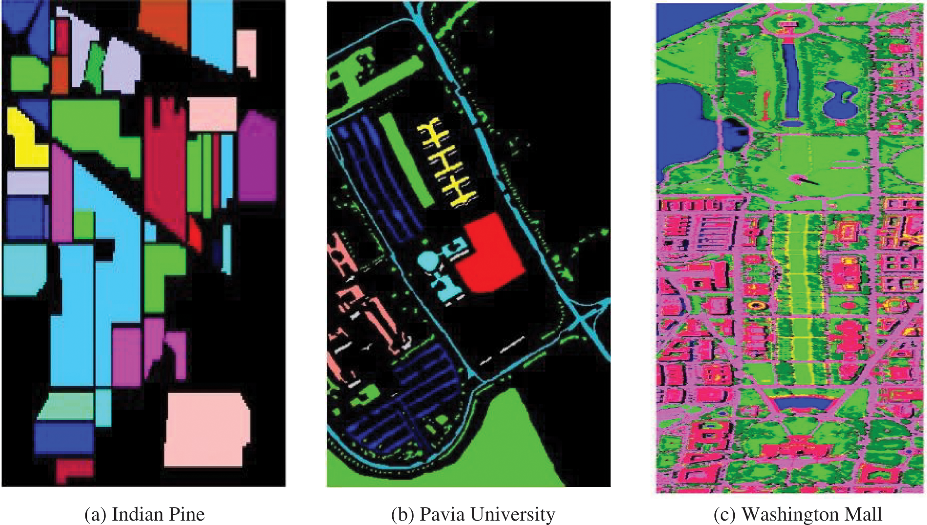
Figure 6: The ground truth of HS datasets: (a) Indian Pines, (b) Pavia University, (c) Washington Mall

The Pavia University dataset, selected as one of the datasets for implementation in this study, offers an insightful example of urban HS imaging. This dataset was captured using the ROSIS sensor over an urban area close to the University of Pavia in Italy. Key characteristics of this HS image include:

•   Pixel Size: The image is composed of pixels measuring 1.3 meters square, providing a detailed view of the urban landscape.

•   Spectral Bands: It contains 103 spectral bands. Each spectral band captures a different wavelength of light, giving a comprehensive spectrum of information about the area imaged.

•   Image Dimensions: The subset of the image used in this study measures 610 by 610 pixels, offering a substantial area for analysis.

A notable aspect of the Pavia University dataset is the need to preprocess the image by removing certain pixels. This is because some parts of the image lack adequate reflectivity information, which is crucial for HS analysis. These areas are typically marked or represented in black in the images, indicating pixels that have been excluded from the dataset due to their lack of information. The dataset is divided into nine distinct classes, each representing a different type of land cover or urban feature. These classes are visually represented in Fig. 6b. The classification of these classes is significant in urban planning and analysis, as it helps in understanding the composition and distribution of various elements in an urban setting.

The Washington Mall HS image dataset refers to a collection of HS images captured over the Washington D.C. Mall area. This dataset is widely used in remote sensing and image processing research, particularly for studies in HS image classification, feature selection, and land cover analysis. Here are the key aspects of this dataset:

•   Data Acquisition and Sensor: The dataset is typically captured using advanced HS sensors like HYDICE. These sensors are capable of capturing images across a wide range of spectral bands, providing detailed information not visible to the naked eye.

•   Spectral Bands: The images in this dataset usually contain a high number of spectral bands, often spanning from 400 to 2400 nanometers (nm). This broad spectrum allows for the detailed analysis of various materials and features present in the urban landscape.

•   Spatial Resolution: The spatial resolution of these images can be quite high. For example, some datasets offer a resolution where each pixel corresponds to a 3-meter area on the ground. This high resolution allows for the detailed examination of features within the urban environment.

•   Area Coverage: The images cover the Washington D.C. Mall, an area with a mix of natural and man-made features. This includes landmarks, green spaces, water bodies, and urban infrastructure. The diversity of this area makes the dataset particularly useful for testing classification algorithms across different types of terrain and objects.

•   Common Usage: Researchers utilize this dataset for various purposes, including but not limited to: Testing and developing new algorithms for HS image analysis, studying urban land cover and land use patterns, conducting environmental monitoring and analysis, and exploring advanced feature extraction methods.

•   Benchmarking and Comparison: Due to its comprehensive and challenging nature, the Washington Mall dataset serves as an excellent benchmark for comparing different image processing techniques and algorithms. It provides a standardized base for researchers to evaluate the effectiveness of their methods.

In summary, the Washington Mall HS image dataset is a valuable resource in the field of remote sensing, offering rich, multi-spectral data that enables detailed analysis and development of sophisticated image processing techniques. Its use in various studies contributes significantly to advancements in HS imaging applications. Fig. 6c shows the ground truth image of Washington Mall dataset.

3  Experimental Results

This section evaluates the efficiency of the MOBGWO-DQL approach in band selection. Its efficacy is gauged using six sophisticated and well-regarded ML algorithms: MOOA, MOBWO, MOGWO, MOGA, RNN, DNN, LSTM, RF, and SVM. For detailed specifics about the calibration settings associated with these algorithms, refer to Table 2. Fine-tuning the parameters of these algorithms is crucial for achieving peak performance. This process involves identifying the best combination of parameter values for the smooth operation of the algorithms. Establishing these optimal configurations is a critical step before proceeding to evaluate the algorithm’s performance.

In this study, we utilize a systematic trial-and-error method for parameter tuning, carefully adjusting each parameter individually and observing its effect while keeping all other variables constant. For example, in an algorithm that involves multiple parameters like learning rates, criteria for convergence, or the size of the population, we examine each parameter in isolation to determine its influence on the algorithm’s performance. To evaluate the effectiveness of these parameter settings, we employ a fitness function, which acts as a metric to assess the algorithm’s output across different parameter configurations. Although the possible variations for each parameter are extensive, practical limitations necessitate the selection and demonstration of a confined set of different parameter scenarios. Table 2 presents this methodology, providing insights into the trial-and-error process by highlighting the parameter values that have either improved or reduced the algorithm’s efficiency in certain cases.

In this study, the analysis of the outcomes was conducted using three key metrics: Accuracy, KC, and RMSE. To compute these criteria, one can refer to Eqs. (14) to (16).

Kappa=N∑i=1rxii−∑i=1r(xi+⋅x+i)N2−∑i=1r(xi+⋅x+i)(14)

RMSE=(1N∑i=1N[Pi−Oi]2)12(15)

Accuracy=TP+TNTP+FN+FP+TN(16)

where r is the number of rows in confusion matrix, xii is entry (i, i) of the confusion matrix, xi+.x+i is the marginal total of column i, row i, respectively, N number of observations, Oi observed parameter, Pi calculated parameter, TP = True positive, FN = False negative, TN = True negative, FP = False positive.

Table 3 indicates the classification accuracy of algorithms for Pavia University dataset. The MOBGWO-DQL exhibits higher class accuracy in the majority of the classes compared to other algorithms. For classes like Asphalt, Meadows, and Gravel, MOBGWO-DQL provides high accuracy rates of 98.41%, 99.32%, and 90.12%, respectively, indicating its effectiveness in correctly classifying these categories. However, the algorithm shows slightly lower accuracy for the Painted Metal Sheets and Bitumen classes, with values of 96.74% and 94.12%, respectively, which are surpassed by MOGWO-DQL, MOBWO-DQL, and MOOA-DQL algorithms in those specific classes. Despite this, MOBGWO-DQL still maintains competitive accuracy rates in these categories. Overall, the MOBGWO-DQL algorithm stands out for its consistent performance, especially when considering the complexity of the dataset, which includes a variety of urban materials and natural elements. Its robustness is particularly notable in classes such as Bare Soil and Self-Blocking Bricks, where it outperforms other algorithms with accuracy rates of 92.27% and 95.71%, respectively. The MOBGWO-DQL has proven to be highly accurate in classifying the majority of the classes within the Pavia University dataset. While it has been outperformed in a couple of classes, its overall performance suggests that it is a strong candidate for effective classification in complex datasets, offering a balance between precision and general applicability across different types of classes.

Table 4 offers a detailed comparative analysis of classification accuracies for different algorithms when evaluated using the Washington Mall dataset. Apart from the category of Trees, the MOBGWO-DQL algorithm exhibits greater accuracy in classification tasks compared to other algorithms. MOBGWO-DQL stands out in its ability to classify numerous classes with higher precision, especially notable in the Water, Grassland, and Street categories, where it consistently achieves top accuracy rates. This underscores MOBGWO-DQL’s exceptional performance in classifying a significant portion of the dataset accurately. Some classes like Water, Grassland, and Tree have high accuracy across all algorithms, suggesting these classes are easier to classify correctly. Other classes like Path, and Shadow have a wider range of accuracies, indicating these may be more challenging to classify. Algorithms like MOBGWO-RNN, MOBGWO-LSTM, MOBGWO-DNN, MOBGWO-RF, and MOBGWO-SVM have some of the lowest accuracies in several classes, indicating they might be less effective for this particular dataset or require further tuning.

Table 5 provides an insightful comparison of class accuracy for various algorithms tested against the Indian Pine dataset. With the exception of corn-Min, corn, Grass/Tree, and stan-steel-to classes, MOBGWO-DQL demonstrates higher precision in classifying than its counterparts. For several classes, MOBGWO-DQL outperforms its counterparts, marking its superiority in accurately classifying the majority of the dataset. This is particularly evident in the classes of Alfalfa, corn-notil, Gross/Pastur, Grass/Pasture, Hay-Windrawed, Oats, Soybeans-nati, Soybeans-clea, Soybean-min, and woods, where MOBGWO-DQL consistently posts higher accuracy percentages. The results imply that the MOBGWO-DQL algorithm is adept at navigating the complexities inherent in the Indian Pine dataset, which could include a wide array of spectral characteristics associated with different crops and natural vegetation.

Table 6 presents the performance metrics of various models on the Indian Pine, Pavia University, and Washington Mall datasets. The metrics used to evaluate model performance include the KC, OA, and RMSE. For the Indian Pine dataset, the MOBGWO-DQL architecture stands out with a KC of 97.68% and an OA of 94.32%, coupled with the lowest RMSE of 0.94. These figures indicate a very high level of agreement between the classifications made by the model and the actual data, with minimal deviation. In comparison, the MOGWO-DQL model shows a decrease in both KC and OA, with a significant increase in RMSE, suggesting less agreement and greater prediction error. The MOOA-DQL, MOBWO-DQL, MOGWO-DQL, and MOGA-DQL models display moderate performance with KCs over 89% and OAs around 86%–90%, but with higher RMSEs, indicating a moderate level of classification error. Notably, as we move down the table to models like MOBGWO-RNN, MOBGWO-LSTM, and MOBGWO-DNN, there is a consistent decline in both KC and OA, along with a substantial rise in RMSE, highlighting a trend of decreasing performance. Turning to the Pavia University dataset, the MOBGWO-DQL model again demonstrates excellent performance, with the highest KC at 98.72% and an impressive OA of 96.01%. It also maintains the lowest RMSE at 0.63, which points to very accurate predictions with minimal error. The remaining models follow a similar trend to that observed with the Indian Pine dataset.

In the Washington Mall dataset, the MOBGWO-DQL achieved the highest accuracy (96.74%). This represents the peak performance of the proposed algorithm across various datasets. Additionally, it boasts the lowest RMSE (0.51) value. The RMSE values are noticeably higher for the Indian Pine dataset across all models except for MOBGWO-DQL, indicating greater prediction errors for this dataset compared to the Pavia University dataset. This could be due to the inherent complexity or the different nature of the Indian Pine dataset, which might present more challenging classification tasks for the models. In assessing the computational efficiency of various algorithms, we average the run times over 20 distinct trials. This average indicates that MOBGWO-DQL outperforms others in terms of speed. The rankings also include MOOA-DQL, MOBWO-DQL, MOGWO-DQL, MOGA-DQL, MOBGWO-RNN, MOBGWO-LSTM, MOBGWO-DNN, MOBGWO-RF, and MOBGWO-SVM algorithms.

Fig. 7 illustrates the comparison of the KC and OA criteria among various algorithms. The MOBGWO-DQL demonstrates superior performance on three datasets, affirming its robustness and effectiveness in HS image classification. The consistent superiority across different metrics suggests that this model can be reliably used for tasks requiring high accuracy and minimal error. According to the results, the use of the DQL architecture for classification yields better outcomes compared to other architectures.

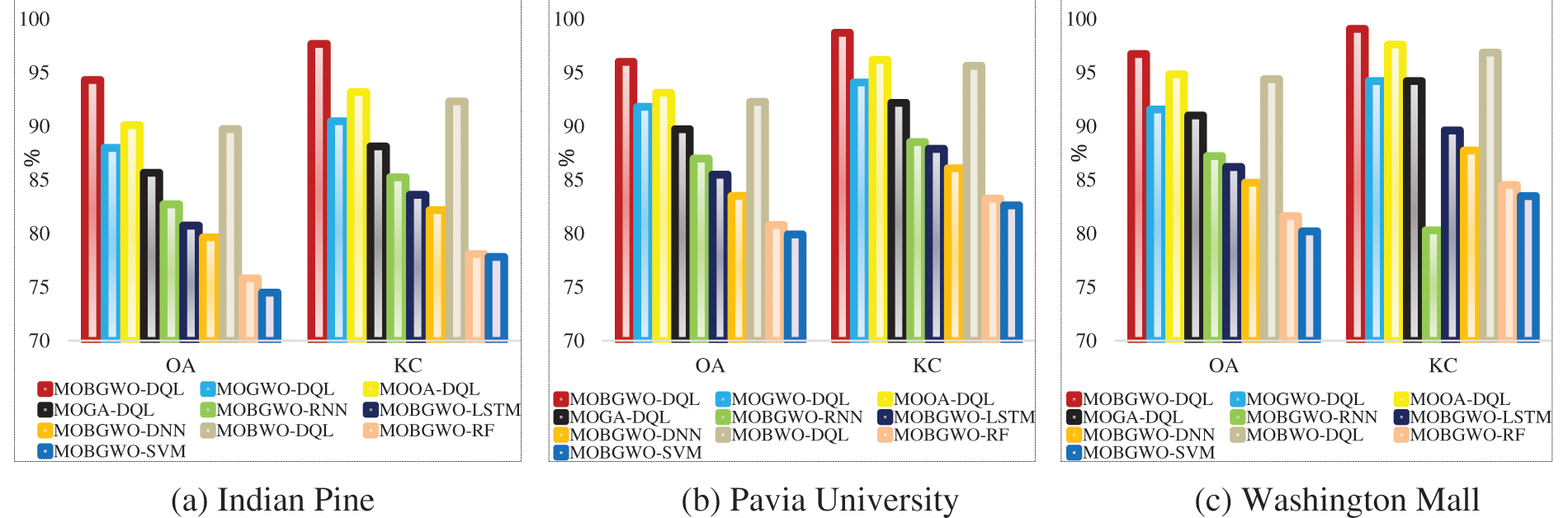
Figure 7: The comparison of algorithms in: (a) Indian Pine, (b) Pavia University, (c) Washington Mall datasets

Table 7 presents comparative results for various ML models with regard to the OA of classifications on three different datasets. The performance is compared across two scenarios based on the ratio of training samples used. From the table, we see that models employing DQL, like MOBGWO-DQL, exhibit relatively stable performance as the training sample size increases. There are improvements, but they are modest compared to the other models. This stability might indicate that DQL-based models can learn effective policies with fewer samples, possibly due to their ability to make better use of sequential decision-making information inherent in the datasets. On the other hand, models such as RNN, LSTM, DNN, RF, and SVM show significant performance improvements as the training samples are increased from 30% to 70%. In conclusion, the results suggest that reinforcement learning algorithms with DQL do not depend heavily on the amount of training data for their performance, unlike traditional ML algorithms. This could be due to the difference in learning paradigms RL models learn policies that generalize across states, while traditional models may need more data to capture the underlying distribution accurately.

Fig. 8 displays a comparative visualization of the ROC curves for various architectures. The examination of the graph in Fig. 8 clearly shows that the area under the curve (AUC) for MOBGWO-DQL, a specific architecture, exceeds that of other architectures. The AUC is an important indicator of a classifier’s overall effectiveness, reflecting the probability that a randomly chosen positive instance will be ranked higher than a randomly chosen negative instance. In this context, the higher AUC associated with MOBGWO-DQL suggests a greater accuracy in classification and a better ability to distinguish between classes compared to the competing architectures.

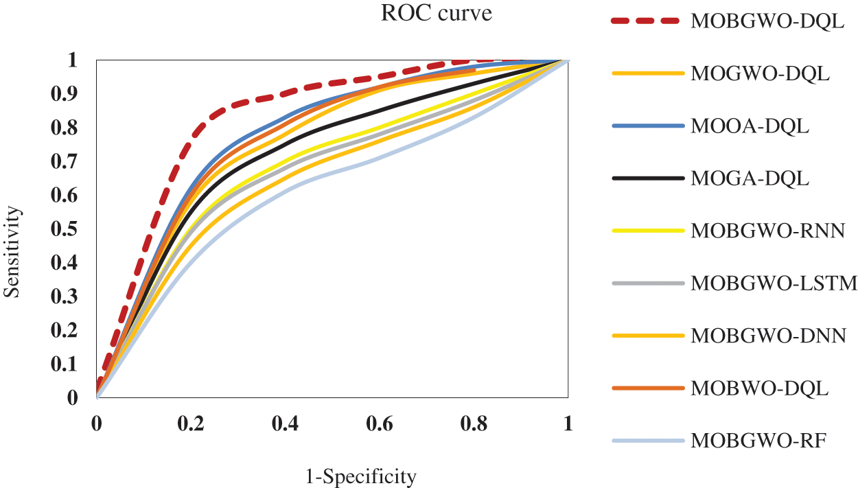
Figure 8: Comparison of the AUC for various models (for Pavia University dataset)

The RMSE criterion is a standard statistical measure used to evaluate the accuracy of a model, particularly in regression analysis and classification. The value of RMSE is always non-negative, and a lower RMSE value indicates a better fit. RMSE is particularly useful because it gives a relatively high weight to large errors. This means that RMSE is sensitive to outliers and can be used to assess the quality of a model in terms of how it handles extreme cases or anomalies. Table 5 clearly indicates that the MOBGWO-DQL architecture surpasses its counterparts, highlighting its superiority for the specific problem at hand. This design’s performance advantage over other architectures underscores its efficacy in addressing the problem. Fig. 9 illustrates the convergence trends of various machine learning architectures in terms of the RMSE over epochs. The MOBGWO-DQL architecture, indicated by the blue line with triangle markers, showcases a leading performance by consistently maintaining the lowest RMSE across all epochs. This suggests that the MOBGWO-DQL architecture not only converges to a more accurate model faster but also sustains its lead in performance throughout the training process. Its sharp decline in RMSE from the outset indicates a robust learning capability, and the maintenance of this low error rate implies excellent generalization over the dataset. In contrast, other architectures, while showing a general trend of improvement, do not reach the low RMSE values exhibited by MOBGWO-DQL. MOBGWO-SVM and MOBGWO-RF, for instance, show a more gradual descent in RMSE, implying a slower learning rate. MOBGWO-LSTM and MOBGWO-RNN also display significant improvements over epochs; however, they plateau at higher RMSE levels compared to MOBGWO-DQL. MOOA-DQL, MOBWO-DQL, MOGWO-DQL, and MOGA-DQL architectures have similar trajectories and demonstrate moderate learning rates. They achieve a respectable reduction in RMSE, but their convergence curves suggest that they might require more epochs to potentially match the performance of MOBGWO-DQL.

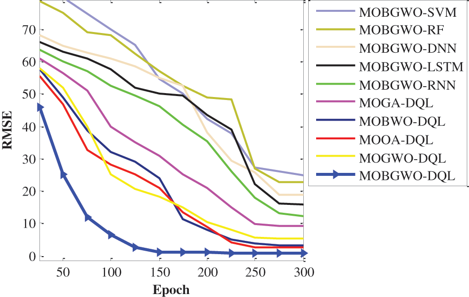
Figure 9: The convergence curve of proposed architectures (for Indian Pine dataset)

4  Conclusion

This paper has presented a novel approach to HS image classification. The key innovation lies in the integration of DQL with a newly developed MOBGWO. This combination aims to optimize band selection in HS images, which is essential for increasing the efficiency and accuracy of image classification. Our experimental results, obtained from publicly available datasets, demonstrate the efficacy of the MOBGWO-DQL algorithm. Compared to other ML models such as LSTM, DNN, RNN, SVM, and RF, our approach shows superior performance in terms of classification accuracy. Specifically, for the Indian Pine dataset, MOBGWO-DQL achieved a KC of 97.68%, an OA of 94.32%, and the lowest RMSE of 0.94. Similarly, for the Pavia University dataset, the model exhibited the highest KC at 98.72%, an impressive OA of 96.01%, and the lowest RMSE at 0.63.

While the MOBGWO-DQL outperforms other methods in most classes, it displays slightly lower OA in certain categories, such as Painted Metal Sheets and Bitumen. Despite this, the algorithm maintains competitive accuracy rates, highlighting its robustness, especially in complex classes such as Bare Soil and Self-Blocking Bricks. Another key observation is the consistent performance of the MOBGWO-DQL across different datasets. The algorithm not only converges to a highly accurate model more quickly but also maintains superior performance throughout the training process. This is evidenced by the lower RMSE values and the sharp decline in error rates from the outset, as seen in the convergence trends.

However, there are limitations and challenges to this approach. The MOBGWO-DQL, while effective, may not be universally superior in all classes, as indicated by its slightly lower performance in specific categories. Additionally, the complexity of datasets like Indian Pine presents a challenge, as indicated by the generally higher RMSE values across models for this dataset compared to Pavia University. Future work should focus on addressing these limitations. Further refinement of the MOBGWO-DQL algorithm could improve its performance in the less accurately classified categories. Additionally, adapting the model to handle the complexities of different datasets more effectively would be beneficial. Investigating the application of this approach in other fields beyond RS, agriculture, and environmental monitoring could also be explored to expand its utility. In conclusion, the MOB-GWO-DQL architecture offers a significant advancement in the field of HS image classification. Its ability to optimize band selection effectively and achieve high accuracy rates makes it a promising tool for various applications. Despite its current limitations, the potential for further improvements and wider applications makes it a valuable contribution to the domain of image classification and ML.

Acknowledgement: The work described in this paper has been developed within the project PRESECREL (PID2021-124502OB-C43). We would like to acknowledge the financial support of the Ministerio de Ciencia e Investigación (Spain), in relation to the Plan Estatal de Investigación Científica y Técnica y de Innovación 2017–2020.

Funding Statement: The authors received no specific funding for this study.

Author Contributions: The authors confirm contribution to the paper as follows: Study conception and design: M. Shoeibi, M. M. Sharifi Nevisi, R. Salehi, D. Martín; data collection: M. Shoeibi, M. M. Sharifi Nevisi, Z. Halimi, S. Baniasadi; analysis and interpretation of results: M. M. Sharifi Nevisi, R. Salehi, Z. Halimi; draft manuscript preparation: M. Shoeibi, D. Martín, S. Baniasadi; supervision: D. Martín. All authors reviewed the results and approved the final version of the manuscript.

Availability of Data and Materials: The datasets generated during and/or analyzed during the current study are available from the corresponding author on reasonable request.

Conflicts of Interest: The authors declare that they have no conflicts of interest to report regarding the present study.

References

1. H. Huang, Z. Liu, C. P. Chen, and Y. Zhang, “Hyperspectral image classification via active learning and broad learning system,” Appl. Intell., vol. 53, no. 12, pp. 15683–15694, 2023. doi: 10.1007/s10489-021-02805-5. [Google Scholar] [CrossRef]

2. B. Alwadei, M. L. Mekhalfi, Y. Bazi, M. M. Al Rahhal, and M. Zuair, “Open set classification of Hyperspectral images with energy models,” Int. J. Remote Sens., vol. 44, no. 24, pp. 7876–7888, 2023. doi: 10.1080/01431161.2023.2288950. [Google Scholar] [CrossRef]

3. X. Dai, W. Lai, N. Yin, Q. Tao, and Y. Huang, “Research on intelligent clearing of weeds in wheat fields using spectral imaging and machine learning,” J. Clean. Prod., vol. 428, pp. 139409, 2023. doi: 10.1016/j.jclepro.2023.139409. [Google Scholar] [CrossRef]

4. M. Kaveh, Z. Yan, and R. Jäntti, “Secrecy performance analysis of RIS-aided smart grid communications,” IEEE Trans. Ind. Inform., vol. 20, no. 4, pp. 5415–5427, 2023. [Google Scholar]

5. F. R. Ghadi, M. Kaveh, and D. Martín, “Performance analysis of RIS/STAR-IOS-aided V2V NOMA/OMA communications over composite fading channels,” IEEE Trans. Intell. Vehicles, vol. 9, no. 1, pp. 279–286, 2023. doi: 10.1109/TIV.2023.3337898. [Google Scholar] [CrossRef]

6. M. Kaveh, M. R. Mosavi, D. Martín, and S. Aghapour, “An efficient authentication protocol for smart grid communication based on on-chip-error-correcting physical unclonable function,” Sustain. Energy Grids Netw., vol. 36, pp. 101228, 2023. [Google Scholar]

7. M. Vahidi, S. Aghakhani, D. Martín, H. Aminzadeh, and M. Kaveh, “Optimal band selection using evolutionary machine learning to improve the accuracy of hyper-spectral images classification: A novel migration-based particle swarm optimization,” J. Classif., vol. 40, no. 3, pp. 1–36, 2023. doi: 10.1007/s00357-023-09448-w. [Google Scholar] [CrossRef]

8. H. Feng, Y. Wang, Z. Li, N. Zhang, Y. Zhang and Y. Gao, “Information leakage in deep learning-based hyperspectral image classification: A survey,” Remote Sens., vol. 15, no. 15, pp. 3793, 2023. doi: 10.3390/rs15153793. [Google Scholar] [CrossRef]

9. W. Sun and Q. Du, “Hyperspectral band selection: A review,” IEEE Geosci. Remote Sens. Mag., vol. 7, no. 2, pp. 118–139, 2019. doi: 10.1109/MGRS.2019.2911100. [Google Scholar] [CrossRef]

10. H. Yang, Q. Du, H. Su, and Y. Sheng, “An efficient method for supervised hyperspectral band selection,” IEEE Geosci. Remote Sens. Lett., vol. 8, no. 1, pp. 138–142, 2010. doi: 10.1109/LGRS.2010.2053516. [Google Scholar] [CrossRef]

11. Q. Wang, F. Zhang, and X. Li, “Optimal clustering framework for hyperspectral band selection,” IEEE Trans. Geosci. Remote Sens., vol. 56, no. 10, pp. 5910–5922, 2018. doi: 10.1109/TGRS.2018.2828161. [Google Scholar] [CrossRef]

12. Q. Wang, Q. Li, and X. Li, “Hyperspectral band selection via adaptive subspace partition strategy,” IEEE J. Sel. Top. Appl. Earth Obs. Remote Sens., vol. 12, no. 12, pp. 4940–4950, 2019. doi: 10.1109/JSTARS.2019.2941454. [Google Scholar] [CrossRef]

13. X. Li et al., “Multi-view learning for hyperspectral image classification: An overview,” Neurocomputing, vol. 500, pp. 499–517, 2022. doi: 10.1016/j.neucom.2022.05.093. [Google Scholar] [CrossRef]

14. D. Ibanez, R. Fernandez-Beltran, F. Pla, and N. Yokoya, “Masked auto-encoding spectral-spatial transformer for hyperspectral image classification,” IEEE Trans. Geosci. Remote Sens., vol. 60, pp. 1–14, 2022. doi: 10.1109/TGRS.2022.3217892. [Google Scholar] [CrossRef]

15. J. Yao et al., “Semi-active convolutional neural networks for hyperspectral image classification,” IEEE Trans. Geosci. Remote Sens., vol. 60, pp. 1–15, 2022. doi: 10.1109/TGRS.2022.3230411. [Google Scholar] [CrossRef]

16. L. Zhao, W. Luo, Q. Liao, S. Chen, and J. Wu, “Hyperspectral image classification with contrastive self-supervised learning under limited labeled samples,” IEEE Geosci. Remote Sens. Lett., vol. 19, pp. 1–5, 2022. [Google Scholar]

17. T. S. Reddy et al., “Hyperspectral image classification with optimized compressed synergic deep convolution neural network with aquila optimization,” Comput. Intell. Neurosci., vol. 2022, pp. 6781740, 2022. [Google Scholar]

18. S. Dhingra and D. Kumar, “Hyperspectral image classification using meta-heuristics and artificial neural network,” J. Inf. Optim. Sci., vol. 43, no. 8, pp. 2167–2179, 2022. doi: 10.1080/02522667.2022.2133222. [Google Scholar] [CrossRef]

19. S. S. Sawant and P. Manoharan, “New framework for hyperspectral band selection using modified wind-driven optimization algorithm,” Int. J. Remote Sens., vol. 40, no. 20, pp. 7852–7873, 2019. doi: 10.1080/01431161.2019.1607609. [Google Scholar] [CrossRef]

20. M. Kaveh and M. S. Mesgari, “Application of meta-heuristic algorithms for training neural networks and deep learning architectures: A comprehensive review,” Neural Process. Lett., vol. 55, pp. 4519–4622, 2022. doi: 10.1007/s11063-022-11055-6. [Google Scholar] [PubMed] [CrossRef]

21. S. Mirjalili, S. M. Mirjalili, and A. Lewis, “Grey wolf optimizer,” Adv. Eng. Softw., vol. 69, pp. 46–61, 2014. doi: 10.1016/j.advengsoft.2013.12.007. [Google Scholar] [CrossRef]

22. M. Kaveh, M. S. Mesgari, D. Martín, and M. Kaveh, “TDMBBO: A novel three-dimensional migration model of biogeogra-phy-based optimization (case study: Facility planning and benchmark problems),” J. Supercomput., vol. 79, no. 9, pp. 1–56, 2023. doi: 10.1007/s11227-023-05047-z. [Google Scholar] [CrossRef]

23. M. Khishe and M. R. Mosavi, “Chimp optimization algorithm,” Expert. Syst. Appl., vol. 149, no. 1, pp. 113338, 2020. doi: 10.1016/j.eswa.2020.113338. [Google Scholar] [CrossRef]

24. H. Yang, M. Chen, G. Wu, J. Wang, Y. Wang and Z. Hong, “Double deep Q-network for hyperspectral image band selection in land cover classification applications,” Remote Sens., vol. 15, no. 3, pp. 682, 2023. doi: 10.3390/rs15030682. [Google Scholar] [CrossRef]

25. M. Kaveh, R. F. Ghadi, R. Jäntti, and Z. Yan, “Secrecy performance analysis of backscatter communications with side information,” Sens., vol. 23, no. 20, pp. 8358, 2023. doi: 10.3390/s23208358. [Google Scholar] [PubMed] [CrossRef]

26. J. Feng et al., “Deep reinforcement learning for semisupervised hyperspectral band selection,” IEEE Trans. Geosci. Remote Sens., vol. 60, pp. 1–19, 2021. [Google Scholar]

27. S. Wang et al., “Deep reinforcement learning enables adaptive-image augmentation for automated optical inspection of plant rust,” Front. Plant Sci., vol. 14, pp. 1142957, 2023. doi: 10.3389/fpls.2023.1142957. [Google Scholar] [PubMed] [CrossRef]

28. L. Mou, S. Saha, Y. Hua, F. Bovolo, L. Bruzzone and X. X. Zhu, “Deep reinforcement learning for band selection in hyperspectral image classification,” IEEE Trans. Geosci. Remote Sens., vol. 60, pp. 1–14, 2021. [Google Scholar]

29. U. Patel and V. Patel, “Active learning-based hyperspectral image classification: A reinforcement learning approach,” J. Supercomput., vol. 80, no. 2, pp. 2461–2486, 2024. doi: 10.1007/s11227-023-05568-7. [Google Scholar] [CrossRef]

30. L. Zhao et al., “Hyperspectral feature selection for SOM prediction using deep reinforcement learning and multiple subset evaluation strategies,” Remote Sens., vol. 15, no. 1, pp. 127, 2022. doi: 10.3390/rs15010127. [Google Scholar] [CrossRef]

31. A. Michel, W. Gross, F. Schenkel, and W. Middelmann, “Hyperspectral band selection within a deep reinforcement learning framework,” in 2020 IEEE Int. Geoscience and Remote Sensing Symp. (IGARSS), Waikoloa, Hawaii, USA, Sep. 2020, pp. 52–55. [Google Scholar]

32. H. Wang, Y. Yuan, X. T. Yang, T. Zhao, and Y. Liu, “Deep Q learning-based traffic signal control algorithms: Model development and evaluation with field data,” J. Intell. Transp. Syst., vol. 27, no. 3, pp. 314–334, 2023. doi: 10.1080/15472450.2021.2023016. [Google Scholar] [CrossRef]

33. B. Arslan and B. Y. Ekren, “Transaction selection policy in tier-to-tier SBSRS by using deep Q-learning,” Int. J. Prod. Res., vol. 61, no. 21, pp. 7353–7366, 2023. doi: 10.1080/00207543.2022.2148767. [Google Scholar] [CrossRef]

34. S. S. Fard, M. Kaveh, M. R. Mosavi, and S. B. Ko, “An efficient modeling attack for breaking the security of XOR-Arbiter PUFs by using the fully connected and long-short term memory,” Microprocess. Microsyst., vol. 94, pp. 104667, 2022. doi: 10.1016/j.micpro.2022.104667. [Google Scholar] [CrossRef]

35. X. Ma, J. Geng, and H. Wang, “Hyperspectral image classification via contextual deep learning,” EURASIP J. Image Video Process, vol. 2015, no. 1, pp. 1–12, 2015. doi: 10.1186/s13640-015-0071-8. [Google Scholar] [CrossRef]

36. S. M. H. Azhdari, A. Mahmoodzadeh, M. Khishe, and H. Agahi, “Pulse repetition interval modulation recognition using deep CNN evolved by extreme learning machines and IP-based BBO algorithm,” Eng. Appl. Artif. Intell., vol. 123, pp. 106415, 2023. doi: 10.1016/j.engappai.2023.106415. [Google Scholar] [CrossRef]

37. M. Kaveh, M. S. Mesgari, and A. Khosravi, “Solving the local positioning problem using a four-layer artificial neural network,” Eng. J. Geospatial Inf. Sci. Eng., vol. 7, no. 4, pp. 21–40, 2020. [Google Scholar]

38. Y. Zhan, D. Hu, H. Xing, and X. Yu, “Hyperspectral band selection based on deep convolutional neural network and distance density,” IEEE Geosci. Remote Sens. Lett., vol. 14, no. 12, pp. 2365–2369, 2017. doi: 10.1109/LGRS.2017.2765339. [Google Scholar] [CrossRef]

39. X. Zhang, T. Lin, J. Xu, X. Luo, and Y. Ying, “DeepSpectra: An end-to-end deep learning approach for quantitative spectral analysis,” Anal. Chim. Acta, vol. 1058, pp. 48–57, 2019. doi: 10.1016/j.aca.2019.01.002. [Google Scholar] [PubMed] [CrossRef]

40. Y. Chen, Z. Lin, X. Zhao, G. Wang, and Y. Gu, “Deep learning-based classification of hyperspectral data,” IEEE J. Sel. Top. Appl. Earth Obs. Remote Sens., vol. 7, no. 6, pp. 2094–2107, 2014. doi: 10.1109/JSTARS.2014.2329330. [Google Scholar] [CrossRef]

41. A. Sellami, M. Farah, I. R. Farah, and B. Solaiman, “Hyperspectral imagery classification based on semi-supervised 3-D deep neural network and adaptive band selection,” Expert. Syst. Appl., vol. 129, pp. 246–259, 2019. doi: 10.1016/j.eswa.2019.04.006. [Google Scholar] [CrossRef]

42. J. Wang et al., “Region-aware hierarchical latent feature representation learning-guided clustering for hyperspectral band selection,” IEEE Trans. Cybern., vol. 53, no. 8, pp. 5250–5263, 2022. doi: 10.1109/TCYB.2022.3191121. [Google Scholar] [PubMed] [CrossRef]

43. C. Tang et al., “Spatial and spectral structure preserved self-representation for unsupervised hyperspectral band selection,” IEEE Trans. Geosci. Remote Sens., vol. 61, pp. 1–13, 2023. doi: 10.1109/TGRS.2023.3331236. [Google Scholar] [CrossRef]

44. M. Vahidi, S. Shafian, S. Thomas, and R. Maguire, “Pasture biomass estimation using ultra-high-resolution RGB UAVs images and deep learning,” Remote Sens., vol. 15, no. 24, pp. 5714, 2023. doi: 10.3390/rs15245714. [Google Scholar] [CrossRef]

45. M. Vahidi, S. Shafian, S. Thomas, and R. Maguire, “Estimation of bale grazing and sacrificed pasture biomass through the integration of sentinel satellite images and machine learning techniques,” Remote Sens., vol. 15, no. 20, pp. 5014, 2023. doi: 10.3390/rs15205014. [Google Scholar] [CrossRef]

46. C. Zhong, G. Li, and Z. Meng, “Beluga whale optimization: A novel nature-inspired metaheuristic algorithm,” Knowl. Based Syst., vol. 251, pp. 109215, 2022. doi: 10.1016/j.knosys.2022.109215. [Google Scholar] [CrossRef]

47. M. Kaveh, M. S. Mesgari, and B. Saeidian, “Orchard algorithm (OAA new meta-heuristic algorithm for solving discrete and continuous optimization problems,” Math. Comput. Simul., vol. 208, pp. 19–35, 2023. doi: 10.1016/j.matcom.2022.12.027. [Google Scholar] [CrossRef]

48. J. Wang, M. Khishe, M. Kaveh, and H. Mohammadi, “Binary chimp optimization algorithm (BChOAA new binary meta-heuristic for solving optimization problems,” Cognitive Computation, vol. 13, pp. 1297–1316, 2021. doi: 10.1007/s12559-021-09933-7. [Google Scholar] [CrossRef]

49. G. G. Devarajan, S. M. Nagarajan, T. V. Ramana, T. Vignesh, U. Ghosh and W. Alnumay, “DDNSAS: Deep reinforcement learning based deep Q-learning network for smart agriculture system,” Sust. Comput.: Informat. Syst., vol. 39, no. 4, pp. 100890, 2023. doi: 10.1016/j.suscom.2023.100890. [Google Scholar] [CrossRef]

50. N. Gholizadeh, N. Kazemi, and P. Musilek, “A comparative study of reinforcement learning algorithms for distribution network reconfiguration with deep Q-learning-based action sampling,” IEEE Access, vol. 11, pp. 13714–13723, 2023. doi: 10.1109/ACCESS.2023.3243549. [Google Scholar] [CrossRef]