Recommendation System Based on Perceptron and Graph Convolution Network

1  Introduction

The Internet has brought great convenience to people, while it has also significantly increased the amount of data, creating information overload. Therefore, people find it challenging to choose the items that best suit their needs. As a significant tool, recommendation systems can address this issue. It performs information filtering, evaluates users’ interests based on past activity, and generates customized recommendations [1]. Recommendation systems are being used extensively in e-commerce, social networking, entertainment, education, and other domains. Well-known applications that rely on recommendation systems have emerged, including WeChat, Taobao, Tmall, and so forth.

Deep learning approaches have recently been widely used in natural language, speech, image, and video [2]. Most conventional recommendation system algorithms use deep learning to extract hidden user and item features from the user ID, comment text, and other data and predict users’ ratings of the item based on these features to provide suggestions. Following its proposal, researchers discovered that the GCN (graph convolution network) was able to extract user-item connection information that was beyond the reach of conventional recommendation algorithms. Using GCN to create recommendation algorithms has gained increasing popularity in today’s recommendation algorithm research.

Presently, most GCN-based recommendation algorithms neglect the unique characteristics of perceptron when extracting user and item features in favor of using the ID of the user’s items to capture user features and then using the matrix correlation operation to determine the user’s score of related items. Inspired by LightGCN [3], we proposed a novel recommendation method called LGAM (LightGCN Attention Mechanism and MLP) is proposed. The proposed method can more effectively integrate higher-order information from user entries, according to experimental data. It not only achieves a better representation of user characteristics but also significantly enhances the effectiveness of recommendations. The main work of this study is as follows:

(1) The proposed LGAM model designed three main modules: The embedding layer, forward propagation layer, and score prediction layer. The LGAM is built upon the foundation of multi-layer perceptron and GCN. Ultimately, the perceptron, adept at capturing user’s interests and preferences, determines the final score.

(2) An attention-integrating GCN is used to implement the forward propagation layer. In order to fully mine the interaction data information between users and items, it can utilize collaborative signals and explicitly encode them in the form of high-order connections by embedded propagation. This reduces both overfitting and data sparsity, better representing user interests and preferences.

(3) Experiments on three standard datasets show that the recall rate and normalized discounted cumulative gain (NDCG) of the proposed LGAM are higher than those of similar algorithms.

2  Related Work

Presently, the techniques for implementing recommendation algorithms mainly include matrix decomposition and deep learning approaches.

2.1 Recommendation Algorithm Basis of Matrix Decomposition

Most conventional recommendation algorithms map users and items to an n-dimensional space using MF (matrix factorization) and then use the mapping to determine the preferences of users for the items—a process known as score prediction. To significantly increase prediction accuracy, recommendation systems, which use MF and biased terms, often use LFM (Latent-Factor Models) [4]. SVD++ (A derivation of the Singular Value Decomposition model) [5] aims to add implicit feedback information based on LFM to correct the prediction results. PMF (Probabilistic Matrix Factorization) model [6] is advanced to improve the missing service score records of the users by updating feature and service feature matrices. Hyper SVD method [7] based on MF using PCA (Principal Component Analysis) for dimensionality reduction is proposed, which is a new method involving the gradual adjustment of the parameters. According to experiment results, the Hyper SVD produces more accurate results than other recommended movies. In order to address the privacy and efficiency challenges faced by MF in collaborative filtering recommendation systems, DS-ADMM (Distributed quantized alternative direction method of multipliers)++ [8] is proposed. DS-ADMM++ integrates differential privacy and utilizes quantized techniques to compress data, which is proven effective by experiments. LSMaOA (Large-Scale Many-Objective Optimization Algorithm) [9] is advanced to improve the MF model for personalized recommendation in the intelligent IoT (Internet of Things). The experimental findings demonstrate the robustness and efficaciousness of LSMaOA in optimizing the six objectives of the model.

2.2 Recommendation Algorithm Basis of Deep Learning

In contrast to deep learning recommendation algorithms, this study investigates GNN (graph neural network), as it can recognize relationships between items and users that deep learning algorithms are unable to. The method basis of neural networks and deep learning is the mainstream direction of recommendation algorithm research. It has been proved that GNN is beneficial for recommendation systems [10]. GCN is one of many GNN implementation techniques that have been widely applied in recommendation systems because of their ability to gradually mine higher-level graph characteristics by adopting multi-layer graph convolution operations [11]. To simulate the high-order relevance of user projects and provide suggestions appropriately, the NGCF (Neural Graph Collaborative Filtering) model [12] is proposed, which introduces GCN into the recommendation algorithm. A-PGNN (A Personalized GNN) [13] is a novel personalized session-aware recommendation approach that primarily combines the Dot-Product attention mechanism and PGNN. Numerous tests demonstrate that A-PGNN performs better than the most advanced related techniques. ExpGCN (Explanation-aware GCN) [14] is advanced and adapted in heterogeneous graph convolutional modeling of recommendation systems, which addresses the limits of computational efficiency and message-passing style. Extensive experiments validate the effectiveness of ExpGCN in explainable recommendations. The attention mechanism is used by the BGANR (Bias-based graph attention neural network recommender) [15] method, which increases the bias term and improves the ability to capture high-order connectivity between nodes. The nia-GCN (Neighbor interaction aware GCN) method [16] takes into account the interaction between neighbor nodes based on GCN, which can effectively collect neighbor node information of all depths. According to the GCN-ONCF (GCN based on Collaborative filtering) model [17], GCN used cross-product operation to convert the coding vector into a two-dimensional feature matrix and a convolution auto-encoder to decompose the convolution matrix. LightGCN, which is based on NGCF, uses a binary graph to reduce the redundant elements of GCN, increasing the model’s effectiveness and performance.

3  LGAM Model Design

3.1 Problem Description and Related Definition

As depicted in Fig. 1, the study’s core task is to train a model according to all the users u interact with all of the items i to learn the relationship in user u, item i, and besides, according to a multi-layer embedding information user u and item i to further get the user u through the MLP layer and characteristic vector of item i, in the end, get score yui.

Figure 1: Model’s core method

The same method is used to yield the u user’s score on all items, and the first K items are recommended to the user u according to the score. The final task is to set the recommendation closer to the u user’s future purchase behavior.

3.2 LGAM Model

3.2.1 LGAM Model Overall Introduction

Taking item i4 and user u1 as examples, the LGAM (LightGCN Attention Mechanism and MLP) model detailed structure is shown in Fig. 2. The model consists of three main modules: Embedding layer, forward propagation layer, and score prediction layer. Modeling users and objects using interaction data is the role of the embedding layer. In the forward propagation layer, ei4(0) and eu1(0) are passed into two parallel GCN with self-connection and weight matrix removed to extract high-order information of user and item, where superscript 0 represents initial embedding. That is the 0 hop expression in the forward propagation layer. Then the final expression of the user and item and ei4 and eu1 is yielded by high-order relation. Lastly, in the score prediction layer, a perceptron extracts the features of the items and users individually. Thus, the prediction score of the user u1 to i4 is calculated, and the score of the user u1 to different items is predicted. According to the prediction score of this set, the first K item contents recommended by the user u1 are given.

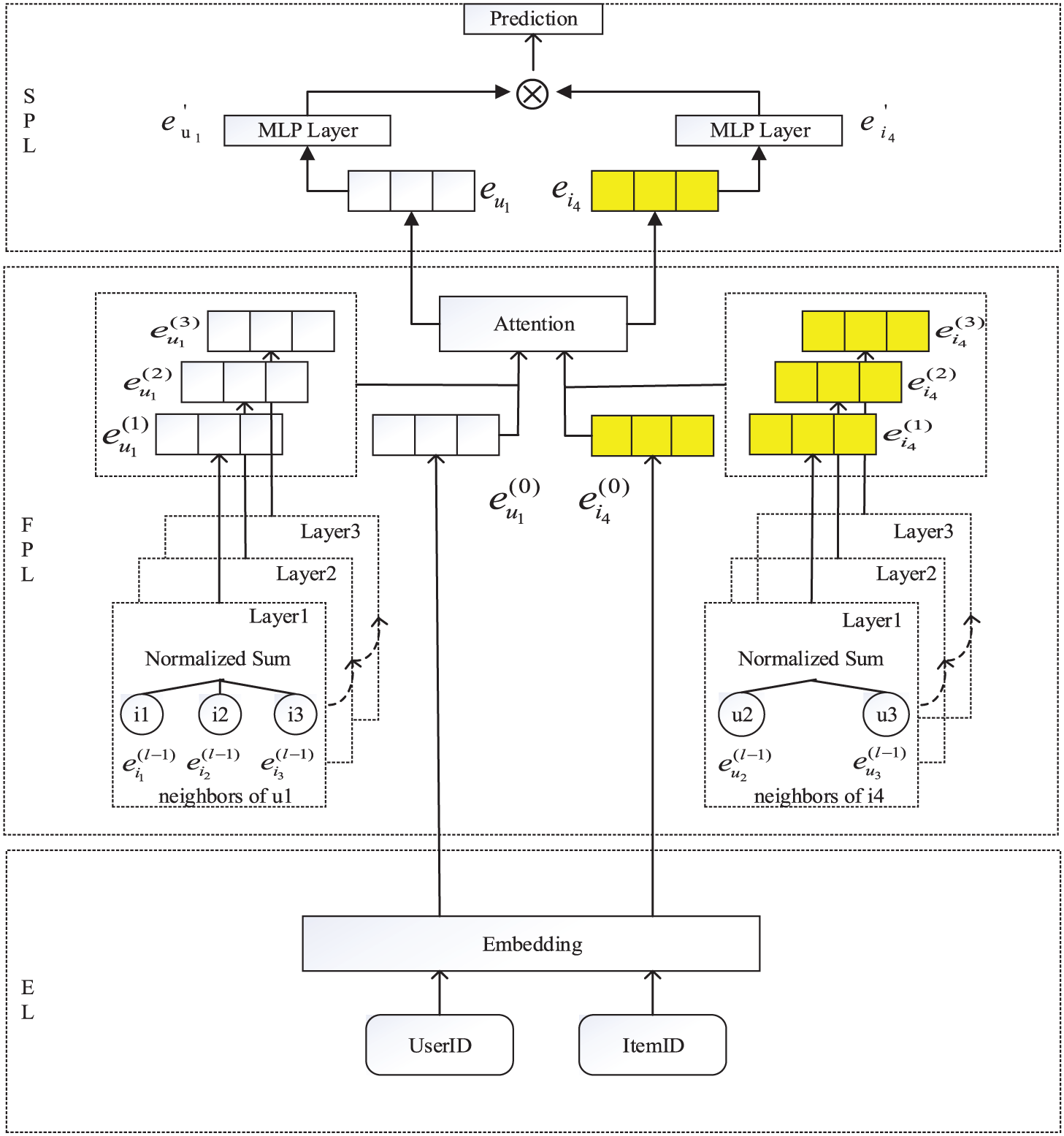
Figure 2: LGAM model structure

3.2.2 Embedded Layer (EL)

The embedding layer is responsible for inputting user and item ID information into the model, and the description of feature embedding is as follows.

Set N users and M items, the ID embedding vector of the ith user is expressed as eui(0)∈Rd, and the ID embedding vector of the jth item is expressed as eij(0)∈Rd, where d is the dimension of the embedding vector, which is a regulable hyperparameter. The ID embedding vector of all users forms a set eu(0)∈RN×d, that is:

eu(0)=[eu1(0),…,eui(0),…,euN(0)](1)

The ID of all items is embedded into the vector to form the set ei(0)∈RM×d, that is:

ei(0)=[ei1(0),…,eij(0),…,eiM(0)](2)

The ID embedding vector of both the item and the user is in the initial state, which is further optimized by the forward propagation layer, which enables the ID embedding vector to convey the association relationship it contains more effectively.

3.2.3 Forward Propagation Layer (FPL)

The forward propagation layer is divided into two parallel frameworks to capture the correlation relation between users and items, respectively.

Suppose the dichotomous graph G of all known associations. The method is similar to LightGCN and extracts the association relation between users and items. Taking user ui and item ij as examples, the calculation rules of user ui’s ID embedded in GCN network to propagate once (i.e., one-hop) are as follows:

eui(1)=∑ij∈Nu1|Nu||Ni|eij(0)(3)

where in eui(1) represents the expression of the first hop of the user ui in GCN network, and eui(0) represents the expression of the zero hop of the item ij, that is the ID embedding of the embedding layer. 1/(|Nu||Ni|) follows the aggregation operation in GCN’s original design, where Nu represents the set of all neighbor nodes that contain user ui, and Ni represents the set of all neighbor nodes that contain the item ij. Eq (3) aggregates the initial ID embedding of all item nodes in all neighbor nodes of the user ui, thereby yielding the embedding expression of the first hop of the user ui in graph convolution. Similarly, the calculation rule for embedding the ID of the item ij in the network is as follows:

eij(1)=∑ui∈Ni1|Nu||Ni|eui(0)(4)

First-order propagation (Eqs. (3) and (4)) of nodes in the GCN network models the features of first-order relevance between users and items. The multi-level graph convolution can be stacked in a GCN network to model the features of high-order correlation between users and items by using the computing method of first-order propagation. It can be inferred that the user ui and item ij perform convolution operations in the forward propagation layer, and the forward propagation rule for the hop from k to k + 1 is defined as follows:

{eui(k+1)=∑ij∈Nu1|Nu||Ni|eij(k)eij(k+1)=∑ui∈Ni1|Nu||Ni|eui(k)(5)

where eui(k+1) and eij(k+1) respectively represent the embedded expression of the (k+1) hop of the user ui and item ij in graph convolution, eui(k) and eij(k) respectively represent the embedded expression of the k-hop of the user ui and item ij in graph convolution operations.

By using the first-order propagation calculation method, stacking multi-layer graph convolution in the GCN network may be used to model the properties of high-order correlation between users and objects. The problem description is depicted in Fig. 3.

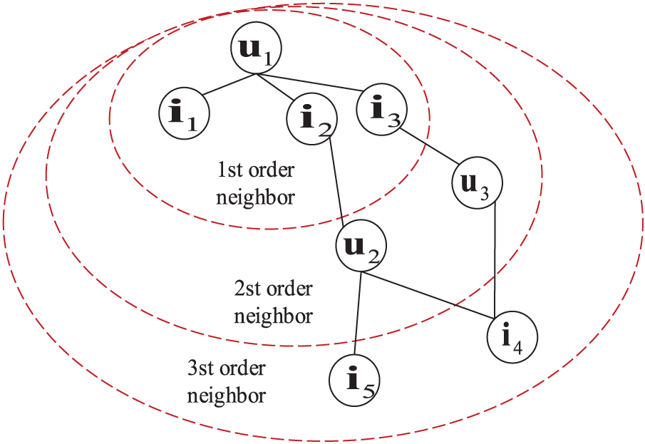
Figure 3: High-level propagation of users and items

User u1 interacts directly with items i1, i2, and i3; Item i2 interacts directly with the user u1 and u2; Item i3 directly interacts with the user u1 and u3, user u2 directly interacts with the item i2, i4 and i5, and user u3 directly interacts with the item i3 and i4.

It can be known from Eq. (5), let 1|Ni||Nu|=P, although the Ni and Nu of each node are different, this does not affect the expression of the formula. This step is only for symbolic convenience and has no specific meaning. Therefore, both are set as P and then the target node u1 is taken as an example to express:

k = 0:

eu1(1)=P(ei1(0)+ei2(0)+ei3(0))(6)

Eq. (6) represents all the direct neighbor relationships between users and items and the items that the user likes.

k = 1:

eu1(2)=P(ei1(1)+ei2(1)+ei3(1))(7)

Eq. (7) represents all the second-order neighbor relationships between the users and the items, such as the item that the user likes being liked by other users.

In the expression of Eqs. (6) and (7), ei1(1)=Peu1(0), ei2(1)=P(eu1(0)+eu2(0)), and ei3(1)=P(eu1(0)+eu3(0)), since the value of P only affects the coefficient and does not affect the relationship between nodes, it is deleted here. Finally, the statement of eu1(2) is as follows:

eu1(2)=P(eu1(0)+eu2(0)+eu3(0))(8)

k = 2:

eu1(3)=P(ei1(0)+ei2(0)+ei3(0)+ei4(0)+ei5(0))(9)

Eq. (8) represents all the third-order neighbor relationships between the users and the items, such as the popular items among users and friends.

Therefore, each additional layer merges the information of the next layer. Attention factor αk is introduced to better extract features. Finally, the expression e^ui of user ui and item ij is obtained, and e^ij is:

{e^ui=∑k=0Kαkeu(k)e^ij=∑k=0Kαkei(k)(10)

where αk≥0 represents the importance of kth layer embedding in forming the final embedding, which can be regarded as the model parameter of automatic optimization. In this experiment, the acquisition of αk using the attentional mechanism results in a satisfactory performance. For user ui, the attention αk∈R1×K of its GCN can be calculated as follows:

αui(k)=softmax(ω1⊗tanh⁡(ω2⊗eui(T)))(11)

Among them, the ω1∈R1×t, ω2∈Rt×d, t is a super parameter that can be adjusted, αuik contains 0 layer to the first k embedded representation of the weight of αui(0) ~ αui(k), softmax () function is used to the weight of k layer embedded normalization.

The weighted sum of embedding vectors of each layer by using the attention vector can yield the final embedding representation eui∈Rd of the correlation relation of user ui:

eui=∑k=0Kαuikeui(k)(12)

Similarly, the embedding representation eij∈Rd of the correlation relation of end-user ij:

eij=∑k=0Kαijkeuij(k)(13)

There are several reasons for the executive-layer composition to achieve the final representation:

(1) The embedding gets excessively smooth as the number of layers rises. Thus, it is challenging to just use the last layer.

(2) Different layers of embedding capture different semantics. As an example, the first layer requires smoothing for users and interactive objects, the second layer smooths users (items) that overlap with users (interactive items), and the higher level records a higher degree of proximity. Therefore, combining them will make the presentation more comprehensive.

(3) The effect of graph convolution and self-connection can be captured by fusing the embeddings of different layers in the form of the weighted sum.

3.2.4 Score Prediction Layer (SPL)

Through the forward propagation layer, the feature vectors eui, eij∈Rd of the association relation between user ui and item ij can be obtained. Then, the vectors eui′ and eij′ of user and item can be yielded through the MLP layer, respectively. Finally, the vector of the user ui is zui ∈Rd, and the calculation of zui is shown as follows:

{z1=ϕ1(eui)z2=α2(W2Tz1+b2)⋯zL−1=αL(WLTzL−2+bL−1)eui′=αL(WLTzL−1+bL)(14)

Similarly, the final form zij ∈Rd of object ij is:

zij=αL(WLTzL−1+bL)(15)

The final score is predicted to be:

y^ui=zui⊗zij(16)

where ϕx denotes the mapping function of the xth layer, WxT represents the characteristic transformation matrix of the xth layer, bx stands for the bias of the xth layer, αx represents the activation function of the xth layer, σ represents the activation function of the output layer, ⊗ represents matrix multiplication, For the activation function of the MLP layer of perceptron, choose sigmoid, hyperbolic tangent (tanh) and Rectifier (ReLU) can also be freely chosen. Each function was analyzed:

1) The sigmoid function constrains each neuron to the range of (0,1), which may limit the performance of the model. It is also prone to overfitting, whereby neurons stop learning when their output approaches zero or one.

2) Tanh is a better choice and has been widely adopted [18,19], but it can only partially alleviate the sigmoid problem because it can be deemed a re-scaled version(tanh(x/2) = 2σ(x) − 1) of sigmoid.

3) Accordingly, ReLU was chosen as the most biologically reasonable [20]. Furthermore, it promotes sparse activation, which works well with sparse data and reduces the likelihood of overfitting in the model. In conclusion, the empirical results demonstrate that the performance of ReLU is marginally better than that of tanh, while tanh significantly outperforms sigmoid. Finally, the activation function used in this paper is ReLU.

3.2.5 Model Optimization

This paper uses BPR [21] loss, which is often applied in recommendation systems, to learn model parameters and improve the model’s ability to express the features of users and items. The foundation of this loss is Bayesian ordering, which considers the relative order of user interactions with objects that are observable and unobservable. It is believed that interactions that are observed have a greater significance than interactions that are not observed. BPR loss is calculated as follows:

Loss=−∑u=1M∑i∈Nu∑j∉Nulnδ(y^ui−y^uj)+λ‖E(0)‖2(17)

where δ denotes the activation function, the sigmoid() function is used, and λ denotes the adjustable regularization coefficient, which controls L2 regularization. The Adam method [22] is used to optimize it and train it with the mini-batch method y^ui denotes the predicted score value of the positive sample, and y^uj denotes the predicted score value of the negative sample.

4  Experimental Analysis

4.1 Preparation

4.1.1 Dataset

To validate the LGAM model, experiments were conducted on three benchmark datasets: Gowalla, Yelp2018, and Amazon-book, which can be open access and differ in domain, size, and sparsity. The statistics for the three datasets are summarized in Table 1.

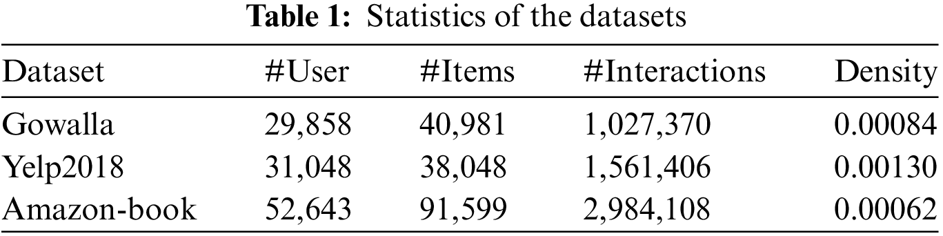
Gowalla: This is the check-in data obtained from Gowalla [23], through which users share their location. To ensure the quality of the data set, 10-core settings were adopted [24], that is, keeping at least 10 interacting users and items.

Yelp2018: This data set was taken from the 2018 version of the Yelp Challenge. Among them, local businesses such as restaurants and bars are considered projects. The same 10-core setup was adopted to ensure data quality.

Amazon-book: Amazon-review is a widely adopted product recommendation data set [25]. Amazon-book was chosen from our collections. Similarly, a 10-core setting was adapted to ensure data quality. For each type of data set, 80% of the historical interaction data of each user was randomly selected as the training set and the rest as the test set. From the training set, 10% of the interactions were randomly selected as the training set to adjust the hyperparameters. For each pair of observed user-item interactions, it was treated as a positive sample. A negative sampling strategy was subsequently performed, pairing it with a negative sample that the user had not previously interacted with.

4.1.2 Evaluation Indicators

For each user in the test set, this article treats all items with which the user does not interact as negative samples. Then, each method outputs the user preference score for all items except the positive sample adopted in the training set. To assess the effectiveness of top-K recommendation and preference ranking, this paper adopted the top-K recommendation method for the recommendation, where K = 20, Recall rate, and NDCG were used to evaluate the model’s performance. Recall is used to evaluate the proportion of the number of interactive items used by users in the list of Top20 recommendations to the number of interactive items used by users in the test set. The Recall rate was directly proportional to a better model effect. Assuming that all user sets in the test set are U, for any user u ∈ U, the recommended list of Top20 is Lu, and the real interaction list of user u in the test set is Lutest, the model recall rate calculation is shown in Eq. (18).

recall@20=∑u∈U1|U||Lu⋂Lutest||Lutest|(18)

The correlation score of the recommendation results at different points in the recommendation list is measured by the NDCG. The higher the ranking, the greater the suggestion effect, and the higher the score of an item, the more relevant it is to the user. Assuming Lui is the recommendation for the ith position in the Top20 recommendation list, f(x) is set to 1 when x > 0, and 0 when vice versa. Set the correlation score rel∈{0,1}, the NDCG calculation method is shown in Eq. (19).

NDCG@20=∑u∈U1|U|DCGu@20IDCGu@20=∑u∈U1|U|∑i=120f(Lu⋂Lutest)log2⁡(i+1)∑i=120f(Lutesti)log2⁡(i+1)(19)

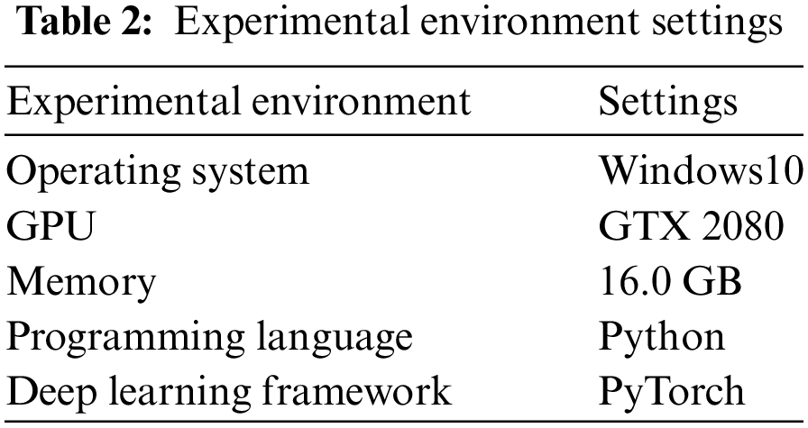
4.1.3 Experimental Environment

GPU can execute high-intensity matrix operations in parallel, completing more computations in the same amount of time because the proposed model requires a lot of computation. GPU is capable of using bigger datasets, increasing training speed, enhancing model performance, and making better use of computational resources. Therefore, this paper chooses to conduct corresponding experimental training on GPU. Table 2 describes the experimental environment settings.

4.2 Compare the Model

The main comparison method is LightGCN, outperforming a variety of methods, including the graph convolutional matrix completion (GC-MC) model [26], PinSage [27], NeuMF basis of the neural network [28], the collaborative memory network model (CMN) [29], factorization-based models MF and Hop-Rec [30]. Comparisons are made under the same assessment criteria as follows:

(1) Mult-VAE [31] is designed based on item-based Collaborative Filtering (CF) and variational automatic coding (VAE), which supposes that data is produced from polynomial distribution and uses variational inference for parameter evaluation.

(2) NGCF successfully integrates GCN into the recommendation system by adhering to the conventional GCN concept. To forecast scores, it effectively extracts embedded interactions (correlation relationships) between users and objects using binary graphs.

(3) Based on NGCF, LightGCN eliminates redundant feature transformation and activation functions, which significantly improves the efficiency and prediction accuracy of the model.

(4) Graph regularized matrix factorization (GRMF) [32] is a way of smoothing matrix decomposition by adding graph Laplacian regularization.

(5) The LII-GCCF (linear transformation, initial residual, identity mapping, graph convolutional collaborative filtering) model [33] is an improved recommendation algorithm using GCN.

4.3 Hyperparameter Adjustment of Experimental Scheme and Model

The embedding size of all models is fixed at 64, and the embedding parameters are initialized by the Xavier method [34]. LGM was optimized using Adam, the default learning rate was 0.001, and the default mini-batch size was 1024 (for Amazon-book data sets, this study increased the mini-batch size to 2048 to improve speed). The L2 regularization coefficient λ is set to 1e-4, and the layer combination coefficient αk is obtained using the attention mechanism. Moreover, an early stop policy is implemented; that is, an early stop occurs if there is no increase in recall@20 on validated data over 50 consecutive epochs.

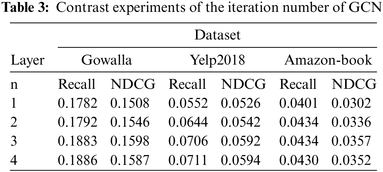
This paper adjusted the graph convolution iteration number n in the experimental part. The dimension of the embedding vector (d = 64) and other parameters in the comparative experiment of varying the number of iterations of graph convolution are consistent with those mentioned previously, as Table 3 illustrates. By examining and comparing the experimental data in Table 3, it can be inferred that the model’s optimal effect is achieved at n = 3. While certain data sets exhibit superior results at n = 4, this will complicate training and limit its benefits, leading to a final iteration number of 3 layers. Considering the sparsity of the data set, it can be inferred that most nodes in the GCN constructed by the three data sets, respectively, have 2-hop and 3-hop paths, and a few have paths above 3-hop (which can be verified by the data set). In this case, more correlations can be extracted when n = 2 than n = 1, and the model impact will be improved. When n = 3, more correlations are extracted than n = 2, which improves the effect of the model. When n = 4, more correlation can be extracted than n = 3; however, the model effect will not be better but will be relatively reduced.

To model the signal of high-order connectivity coding, the depth of high-order relevance in LGAM is set as 3, and the layer number of perceptron MLP is set as 2. This article presents the findings of three embedded propagation layers with a 0.1 message loss rate and a 0.0 node loss rate without any more explanation. Typically, the model can converge after 1000 epochs.

4.4 Performance Comparison

Table 4 demonstrates that LGAM outperforms alternative approaches across all data sets. Its efficiency is evidenced by a straightforward and rational design, where the model’s best outcomes are bolded.

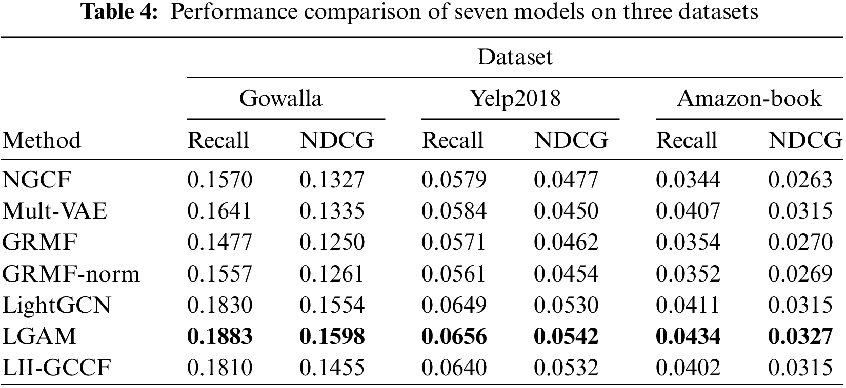
The performance of GRMF is comparable to that of NGCF. GRMF-norm outperforms GRMF on Gowalla and adds little value on Yelp2018 and Amazon-book by normalizing the Laplacian regularizer. Because of the non-linear interaction between user and object features during feature extraction and the addition of a perceptron, the LGAM model performs marginally better than the LightGCN model.

As can be seen from the above Table 4:

(1) LGAM outperforms slightly than LightGCN, and LightGCN is marginally superior to other methods. For instance, on Gowalla, the highest recall rate recorded in the LightGCN is 0.1830; however, in this study, the NDCG is 2.83% higher, and the LGAM can reach 0.1883 in a 3-layer setting, which is 2.90% higher. For example, the results of LGAM on the Gowalla dataset are shown in Fig. 4.

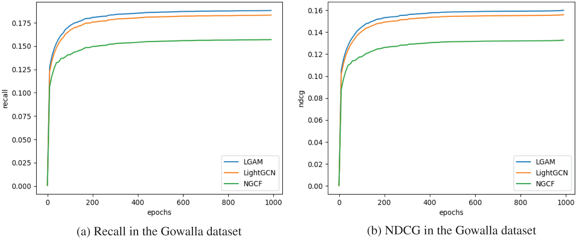
Figure 4: Evaluation metrics on the Gowalla dataset

(2) Raising the number of layers improves performance but reduces the benefits. The usual observation is that raising the number of layers from 0 to 1 results in maximum performance gain and adopting the number of layers three results in satisfactory performance in most cases.

(3) LGAM consistently produced reduced training loss during the training process, effectively translating to improved test accuracy and demonstrating LGAM’s potent generalization capacity. Although improving the learning rate of LightGCN can reduce its training loss, it cannot improve the test recall rate because reducing training loss is only a temporary solution for LightGCN.

4.5 Ablation Experiment

Ablation tests were performed to validate the efficacy of the LGAM model further. The hyperparameter adjustment discussed in Section 4.3 is consistent with the parameters of the LGAM model without an attention mechanism, which we will refer to as LGM. The graph convolution iteration number is 3. The comparison results of the LGM model’s recall rate and NDCG on the Gowalla dataset are shown in Fig. 5. Thus, it can be concluded that the attention mechanism has a positive effect on the model. In terms of recall, LGAM has improved by 1.074% compared to LGM, and the normalized cumulative loss gain of this model has increased by 2.04% compared to LGM.

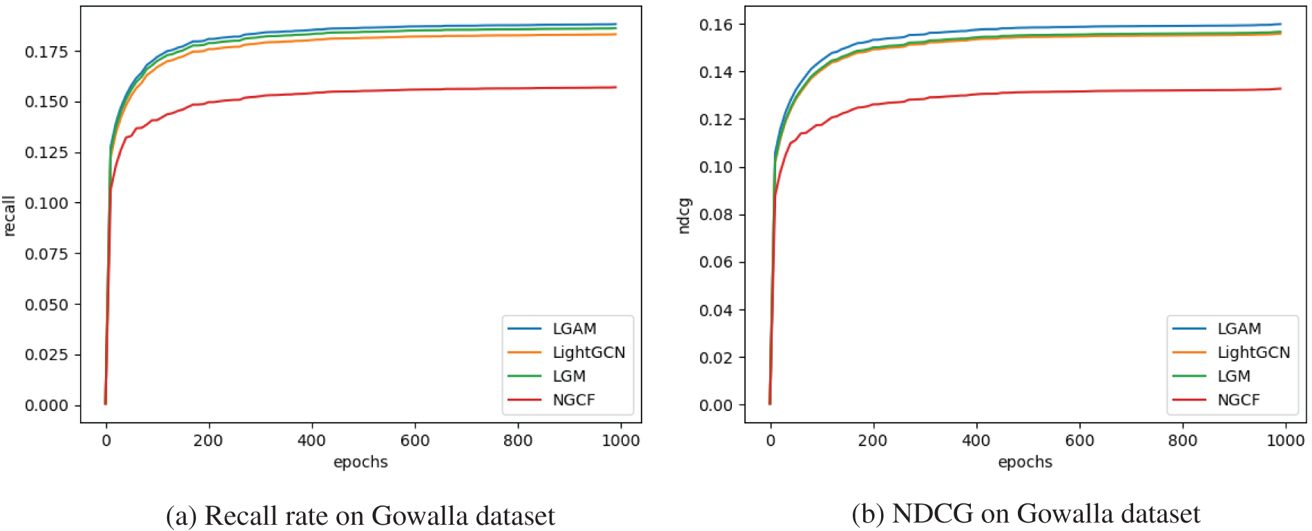
Figure 5: Ablation experiment on the Gowalla dataset

5  Conclusion

To fully extract the features of users’ items, this study proposes a hybrid algorithm known as LGAM. The model combines the strengths of graph neural networks and attention mechanism, consisting of closely related modules: EL, FPL, and SPL; notably, the FPL plays a crucial role. It employs two parallel GCNs to simultaneously extract the features from users and items. By stacking multi-layer graph convolutions and incorporating a carefully designed attention factor, it effectively captures higher-order correlations and association relevance information between users and items, better expressing user interests and preferences.

Experimental results on three datasets show that LGAM achieves higher recall and NDCG compared to other methods. This indicates its effectiveness in enhancing recommendation performance. In the future, frameworks such as knowledge graphs and neighborhood aggregation may be explored to optimize the model further. Additionally, the study will delve into the impacts of different feature fusions on the recommendation system.

Acknowledgement: None.

Funding Statement: This work was supported by the Fundamental Research Funds for Higher Education Institutions of Heilongjiang Province (145209126) and the Heilongjiang Province Higher Education Teaching Reform Project under Grant No. SJGY20200770.

Author Contributions: Writing—review and editing, supervision and funding acquisition: Z. Lian; validation and writing—original draft: Y. Yin; conceptualization, methodology, and formal analysis: H. Wang. All authors reviewed the results and approved the final version of the manuscript.

Availability of Data and Materials: The data used in the study are all available.

Conflicts of Interest: The authors declare that they have no conflicts of interest to report regarding the present study.

References

1. J. Yao, “Review of personalized recommendation system,” China Collect. Econ., no. 25, pp. 71–72, 2020. [Google Scholar]

2. Y. LeCun, Y. Bengio, and G. Hinton, “Deep learning,” Nature, vol. 521, no. 7553, pp. 436–444, 2015. doi: 10.1038/nature14539. [Google Scholar] [PubMed] [CrossRef]

3. X. He, K. Deng, X. Wang, and Y. Li, “LightGCN: Simplifying and powering graph convolution network for recommendation,” in Proc. 43rd Int. ACM SIGIR Conf. Res. Dev. Inf. Retriev., Xi’an, China, 2020, pp. 639–648. [Google Scholar]

4. Y. Deldjoo, T. D. Noia, and F. A. Merra, “A survey on adversarial recommender systems,” ACM Comput. Surv., vol. 54, no. 2, pp. 1–38, 2022. doi: 10.1145/3439729. [Google Scholar] [CrossRef]

5. M. Jallouli, S. Lajmi, and I. Amous, “When contextual information meets recommender systems: Extended SVD++ models,” Int. J. Comput. Appl., vol. 44, no. 4, pp. 349–356, 2020. doi: 10.1080/1206212X.2020.1752971. [Google Scholar] [CrossRef]

6. L. Duan, T. Gao, W. Ni, and W. Wang, “A hybrid intelligent service recommendation by latent semantics and explicit ratings,” Int. J. Intell. Syst., vol. 36, no. 2, pp. 7867–7894, 2021. doi: 10.1002/int.22612. [Google Scholar] [CrossRef]

7. B. Geluvaraj and M. Sundaram, “A Matrix factorization technique using parameter tuning of singular value decomposition for recommender systems,” Turk. J. Comput. Math. Educ., vol. 12, no. 2, pp. 3313–3319, 2021. [Google Scholar]

8. F. Zhang, E. Xue, R. Guo, G. Qu, G. Zhao and A. Y. Zomaya, “DS-ADMM++: A novel distributed quantized ADMM to speed up differentially private matrix factorization,” IEEE Trans. Parallel Distrib. Syst.: Publ. IEEE Comput. Soc., vol. 33, no. 6, pp. 1289–1302, 2022. doi: 10.1109/TPDS.2021.3110104. [Google Scholar] [CrossRef]

9. B. Cao, Y. Zhang, J. Zhao, X. Liu, and Z. Lv, “Recommendation based on large-scale many-objective optimization for the intelligent internet of things system,” IEEE Internet Things J., vol. 9, no. 16, pp. 15030–15038, 2021. doi: 10.1109/JIOT.2021.3104661. [Google Scholar] [CrossRef]

10. Y. Guo, Y. Ling, and H. Chen, “A time-aware graph neural network for session-based recommendation,” IEEE Access, vol. 8, pp. 167371–167382, 2020. doi: 10.1109/ACCESS.2020.3023685. [Google Scholar] [CrossRef]

11. J. Chen, G. Lin, J. Chen, and Y. Wang, “Towards efficient allocation of graph convolutional networks on hybrid computation-in-memory architecture,” Sci. China: Inf. Sci., vol. 64, no. 6, pp. 108–121, 2021. doi: 10.1007/s11432-020-3248-y. [Google Scholar] [CrossRef]

12. X. Wang, X. He, M. Wang, F. Feng, and T. S. Chua, “Neural graph collaborative filtering,” in Proc. 42nd Int. ACM SIGIR Conf. Res. Dev. Inf. Retriev., Paris, France, 2019, pp. 165–174. [Google Scholar]

13. M. Zhang, S. Wu, M. Gao, X. Jiang, K. Xu and L. Wang, “Personalized graph neural networks with attention mechanism for session-aware recommendation,” IEEE Trans. Knowl. Data Eng., vol. 34, no. 8, pp. 3946–3957, 2022. doi: 10.1109/TKDE.2020.3031329. [Google Scholar] [CrossRef]

14. T. Wei, T. W. S. Chow, J. Ma, and M. Zhao, “ExpGCN: Review-aware graph convolution network for explainable recommendation,” Neural Netw., vol. 157, no. 9, pp. 202–215, 2023. doi: 10.1016/j.neunet.2022.10.014. [Google Scholar] [PubMed] [CrossRef]

15. J. Wang, Q. Wen, X. Yang, and Q. Zhang, “Recommended attention neural networks algorithm based on deviation,” Control Decis., vol. 37, no. 7, pp. 1705–1712, 2020. [Google Scholar]

16. J. Sun et al., “Neighbor interaction aware graph convolution networks for recommendation,” in Proc. 43rd Int. ACM SIGIR Conf. Res. Dev. Inf. Retriev., Xi’an, China, 2020, pp. 1289–1298. [Google Scholar]

17. J. Su, T. Xu, X. Zhang, Y. Shi, and S. Gu, “Collaborative filtering recommendation based on convolution and outside product model,” Comput. Appl. Res., vol. 38, no. 10, pp. 3044–3048, 2021. [Google Scholar]

18. M. A. Mercioni and S. Holban, “Developing novel activation functions in time series anomaly detection with LSTM autoencoder,” in Proc. 2021 IEEE 15th Int. Symp. Appl. Comput. Intell. Inf. (SACI), Timişoara, Romania, 2021, pp. 000073–000078. [Google Scholar]

19. R. Gnanasambandam, B. Shen, J. Chung, X. Xue, and Z. Kong, “Self-scalable Tanh (StanFaster convergence and better generalization in physics-informed neural networks,” arXiv:2204.12589, 2022. [Google Scholar]

20. L. L.Parisi, D. Neagu, R. Ma, and F. Campeanet, “Quantum ReLU activation for convolutional neural networks to improve diagnosis of Parkinson’s disease and COVID-19,” Expert Syst. Appl., vol. 187, no. 1, pp. 115892, 2022. [Google Scholar]

21. S. Rendle, C. Freudenthaler, Z. Gantner, and L. Schmidt-Thiemeet, “BPR: Bayesian personalized ranking from implicit feedback,” arXiv:1205.2618, 2012. [Google Scholar]

22. D. P. Kingma and J. Ba, “Adam: A method for stochastic optimization,” arXiv:1412.6980, 2014. [Google Scholar]

23. D. Liang, T. McInerney, and D. Terzopoulos, “Modeling user exposure in recommendation,” in Proc. 25th Int. Conf. World Wide Web, 2016, pp. 951–961. [Google Scholar]

24. R. He and J. McAuley, “VBPR: Visual Bayesian personalized ranking from implicit feedback,” in Proc. 30th AAAI Conf. Artif. Intell., Phoenix, USA, vol. 30, 2016, pp. 1–7. [Google Scholar]

25. R. He and J. McAuley, “Ups and downs: Modeling the visual evolution of fashion trends with one-class collaborative filtering,” in Proc. 25th Int. Conf. World Wide Web, arXiv:1602.01585, 2016. [Google Scholar]

26. R. Berg, T. Kipf, and M. Welling, “Graph convolutional matrix completion,” in Proc. KDD’18 Deep Learn. Day, London, UK, 2017, pp. 1–7. [Google Scholar]

27. R. Ying, R. He, K. Chen, P. Eksombatchai, W. L. Hamilton, and J. Leskovec, “Graph convolutional neural networks for web-scale recommender systems,” in Proc. 24th ACM SIGKDD Int. Conf. Knowl. Discov. Data Min., London, UK, 2018, pp. 974–983. [Google Scholar]

28. X. He, L. Liao, H. Zhang, L. Nie, and T. S. Chua, “Neural collaborative filtering,” in Proc. 26th Int. Conf. World Wide Web, Perth, Australia, 2017, pp. 173–182. [Google Scholar]

29. T. Ebesu, B. Shen, and Y. Fang, “Collaborative memory network for recommendation systems,” in 41st Int. ACM SIGIR Conf. Res. Dev. Inf. Retriev., Ann Arbor, USA, 2018, pp. 515–524. [Google Scholar]

30. J. H. Yang, C. M. Chen, C. J. Wang, and M. F. Tsai, “HOP-rec: High-order proximity for implicit recommendation,” in Proc. 12th ACM Conf. Recommender Syst., Vancouver, Canada, 2018, pp. 140–144. [Google Scholar]

31. D. Liang, R. G. Krishnan, M. D. M.D.Hoffman, and T. Jebara, “Variational autoencoders for collaborative filtering,” in Proc. 2018 World Wide Web Conf., Lyon, France, 2018, pp. 689–698. [Google Scholar]

32. N. Rao, H. F. Yu, P. K. Ravikumar, and I. S. Dhillon, “Collaborative filtering with graph information: Consistency and scalable methods,” Adv. Neural Inf. Process. Syst., vol. 28, pp. 1–9, 2015. [Google Scholar]

33. R. Guo, X. Li, Y. Hu, and M. Qu, “A simple graph convolutional network with abundant interaction for collaborative filtering,” IEEE Access, vol. 9, pp. 77407– 77415, 2021. doi: 10.1109/ACCESS.2021.3083600. [Google Scholar] [CrossRef]

34. X. Glorot and Y. Bengio, “Understanding the difficulty of training deep feedforward neural networks,” in Proc. 13th Int. Conf. Artif. Intell. Stat., Sardinia, Italy, 2010, pp. 249–256. [Google Scholar]