Fault Diagnosis Method of Rolling Bearing Based on MSCNN-LSTM

1  Introduction

Rolling element bearing, as a key basic mechanical component widely used in modern industries, is prone to various forms of defects due to the complex and variant working conditions, which will affect the efficiency of mechanical equipment, spawn pecuniary losses and even threaten personal safety [1–4]. Therefore, fault diagnosis of bearing has raised great interest in the academic and industrial domains [5,6].

As an important branch of machine learning, deep learning technology [7] has broadened its application scope recently, such as driverless cars [8,9] computer vision [10,11], etc. Naturally, in bearing fault diagnosis area, various deep networks, including deep belief networks [12], autoencoder [13], recurrent neural networks [14], especially convolutional neural networks [15], etc., have been developed more and more and achieved remarkable results [16].

A critical component of the safe operation of mechanical equipment is the identification of rolling bearing faults. The main goal of rolling bearing fault recognition is to find, diagnose, and pinpoint the source of the vibration data collected from the bearings by using a variety of effective signal processing algorithms.

While time domain analysis is easy to use and straightforward, the fault information derived from statistical parameters that are explicitly chosen is not all-inclusive and has limitations. Fault diagnosis is done using spectral analysis, while frequency domain analysis is based on processed signals in the frequency domain. Amplitude, power, energy, envelope, and other types of spectra are frequently utilized. Zhang et al. [17] proposed an improved integrated empirical mode decomposition hard threshold denoising method, which denoises the collected data and highlights the fault characteristics of each sensor. Secondly, the Gaussian mixture model was used to analyze single-source and multi-source faults of sensors at different points. The experimental results indicate that the Gaussian mixture model and Gaussian mixture model have high diagnostic ability. Chen et al. [18] employed optimization algorithms to enhance the classification accuracy of support vector machines by optimizing parameters. The chicken swarm optimization algorithm, a novel global optimization approach proposed in recent years, is widely utilized for solving optimization problems due to its clear structure and robust global search capability. Building upon this foundation, we propose a fault diagnosis method based on the chicken swarm optimization support vector machine model and apply it to the bearing fault diagnosis field, comparing it with the trained model to determine the fault type. Han et al. [19] presented a cyclostationary analysis and variational mode decomposition-based defect diagnosis technique for rolling bearings. Initially, the correlation coefficient index is used to adaptively determine the suitable mode number of various signals. The determined mode number is then used to break down the original signals using variational mode decomposition, yielding certain intrinsic mode components. Second, select the optimal IMF based on the maximum kurtosis criterion. Finally, the best intrinsic mode components are picked out, and they are given a more thorough envelope spectrum analysis based on cyclostationary analysis.

While there have been some successes with this kind of approach, its use is severely constrained by its high reliance on expert knowledge, laborious feature extraction process, and subpar generalization capabilities; It will also be important for the model to adaptively extract features since, over the course of the mechanical equipment detection system’s extended operation, the amount of state detection data will grow.

As artificial intelligence and other technologies have advanced in recent years, deep learning has been progressively used in the field of fault diagnostics. When it comes to retrieving feature information that characterizes bearing states from huge amounts of data, deep learning makes up for the drawbacks of shallow network models. Rather than requiring a manual feature extraction method, the deep network structure of deep learning may directly extract features from the original vibration signals of bearings. Inspired by the above research, many researchers are interested in developing deep network-based artificial intelligence algorithms in bearing fault diagnosis [20–23]. For instance, Lu et al. [24] presented a deep neural network embedding maximum mean discrepancy for cross-domain bearing fault identification. Li et al. [25] addressed the bearing fault diagnosis domain shift problem by minimizing multi-layer and multi-kernel maximum mean discrepancies between two domains. While the techniques can successfully extract fault feature information, it is challenging to recover temporal information from vibration signals when depending just on convolutional structures since vibration signals have certain temporal features and periodicity.

Numerous research studies have indicated that even though one system consistently exhibits better performance than another, the combined utilization of both systems has the potential to achieve superior results [26]. Mwelinde et al. [27] proposed an integrated model based on Hierarchical Fuzzy Entropy, Convolutional Neural Network and Long Short-Term Memory. The two main components of the model are fault classification and feature extraction. Furthermore, to improve the computational efficiency and classification accuracy of the model, an intensity discriminator is integrated into the convolutional neural network to efficiently extract critical features that represent the actual condition of the bearing. Therefore, Liao et al. [28] proposed a bearing fault diagnosis method based on CNN-BiLSTM-Attention. This technique combines a bidirectional long-short-term memory network with a convolutional neural network. It then adds a dropout mechanism to the BiLSTM network to prevent overfitting. Finally, it adds an attention mechanism to automatically assign different weights to the BiLSTM network to enhance its sensitivity and its capacity to understand various fault information.

Even though these techniques show off CNN’s benefits, there are still issues such limited generalization, insufficient convolutional kernel scale, trouble adequately extracting deep fault characteristics, and challenges maintaining excellent performance in the face of heavy noise and fluctuating loads.

Although deep learning techniques have advanced significantly in the field of fault identification thus far, certain issues remain. Firstly, stacking convolutional layers is typically used to improve network performance for the problem of challenging extraction of bearing defect characteristics. However, this increases the spatial complexity of the network and complicates the deployment of the model. Second, the model’s stability and dependability may suffer if the coupling effect between noise interference and load variations is ignored. Lastly, it is challenging to acquire real defect samples and to attain optimal network performance.

To address the problems, the multi-scale fusion module was employed to enhance CNN’s learning process, successfully extracting the data’s essential fault space feature information. An LSTM network was combined to create a fusion network model that fully extracted temporal features. This paper employs long-short-term memory networks to enhance feature extraction efficacy and presents a fault diagnostic technique based on these networks along with convolutional and long-short-term memory networks. In this study, multiple techniques are implemented to ensure the model’s complexity while minimizing the phenomena of excessive fitting, including the addition of a BN layer and a dropout layer. Ultimately, a completely connected layer completes the bearing status recognition and categorization process.

2  Theoretical Backgrounds

2.1 Convolutional Neural Network

The convolutional neural network (CNN), a kind of deep neural network with a convolution structure, has been widely used in many practical applications and achieved impressive performance. The architecture of CNN is composed of the input layer, convolutional layer, pooling layer, fully connected layer, and output layer. In general, a convolutional layer consists of multiple kernels. It convolves the raw input data with kernels and generates features. The output of the layer can be expressed as:

xjl=δ(∑ixil−1∗Wjl+bjl)(1)

where xil−1 denoted the i−th feature map in the l−1 layer; Wjl represents the j−th kernel in the layer l; bjl denotes the bias; ∗ is the convolutional calculation; δ(⋅) indicates the activation function, and the rectified linear unit (ReLU) is selected in this work. The formula can be defined as follows:

δ(xms)=max(xms,0)(2)

After the activation operation, the deep features are flattened into one-dimensional vectors, then a fully connected layer is utilized to conduct classification. The pooling layer’s primary job is to carry out down-sampling operations, which clean up the input feature vector’s features to extract the key attributes. This method’s primary goal is to make neural network parameters less computationally tricky. By doing so, overfitting issues can be prevented more successfully. But in this paper, global average pooling is first proposed to replace the fully connected layer to enhance generalization ability.

2.2 Long-Short-Term Memory Network

In 1997, Hochreiter and Schmid Huber proposed long-short-term memory networks (LSTM). These networks introduced gating units and memory mechanisms to improve feature extraction capability. This effectively addressed the issue of gradient vanishing and prevented RNN from losing its capacity to learn new information. Most of RNN’s features are carried over to LSTM. It is superior to RNN in processing lengthy sequence signal data and has a stronger memory.

As shown in Fig. 1, by adding input, forgetting, and output gates, this model functions as a gated neural network and processes data. The input gate’s primary function is to evaluate incoming data and determine how much of it may now be saved to the memory unit; The forgetting gate primarily regulates the updating and forgetting of data in the memory unit, deciding which historical data should be forgotten and which data should be kept; in other words, it determines how the previous time memory unit affected the current time memory unit; The output gate determines how the memory unit affects the current output value by controlling the LSTM unit’s output at that moment. The three gate control units that have been introduced work together to store and update data through the LSTM, and the gate control unit’s hidden layer is fully connected.

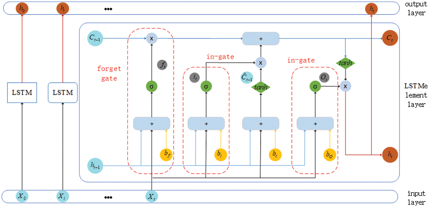
Figure 1: Architecture for long-short-term memory network

The following formula can represent the gate’s output:

ft=σ(Wf⊙[ht−1,Xt]+bf)(3)

in the formula, Wf and bf stand for weights and biases; The product of the elements is represented by the operator; The sigmoid activation function is represented by σ, whose output is 1 when the value is retained and 0 when it is forgotten.

Two activation functions are employed to ascertain the data kept in the state unit of an LSTM. The input gate’s sigmoid function determines the information to be updated, and the new information to be added to the unit state denoted by Ct is determined by the hyperbolic tangent function. The following is the mathematical description:

it=σ(Wi⊙[ht−1,Xt]+bi)(4)

Ct=tanh⁡(WC⊙[ht−1,Xt]+bC)(5)

it=σ(Wi⊙[ht−1,Xt]+bi)(6)

The input gate’s output is represented by it in the formula; the weights and biases of the input gates are represented by Wi and bi; the consequences and preferences of the tanh function are represented by WC and bC, respectively.

Meanwhile, Wf stand for weights, the LSTM unit calculates the output Ot of the output gate using the following equation:

Ot=σ(WO⊙[ht−1,Xt]+bO)(7)

Finally, calculate the output ht of the hidden layer unit as follows:

ht=Ottanh⁡(Ct)(8)

3  Proposed Methods

3.1 Framework of MSCNN-LSTM

An LSTM module plus a CNN module make up the entire model. While conventional CNN models can extract shape properties from the original bearing vibration signals, they struggle to capture the temporal elements of the signs, which leads to the loss of essential features in the time series. With the use of unique gating mechanisms, LSTM can learn temporal aspects of vibration signals and address problems closely tied to time. In the meantime, multi-scale can reduce superfluous features, enhance the expression ability of significant characteristics, and dynamically assign weights to input elements. As a result, it has been suggested to use a rolling bearing fault diagnosis technique based on the combination of long short-term memory networks and convolutional neural networks (MSCNN-LSTM).

This paper presents a method that allows neural networks to determine the rolling bearing health condition by directly extracting internal feature representations from normalized vibration data. The MSCNN-LSTM model’s structure is depicted in Fig. 2. Z-score normalization is applied to all samples before training to standardize dimensions and make further computations easier. A raw time-domain signal with a length of 1,1024 is the input sample.

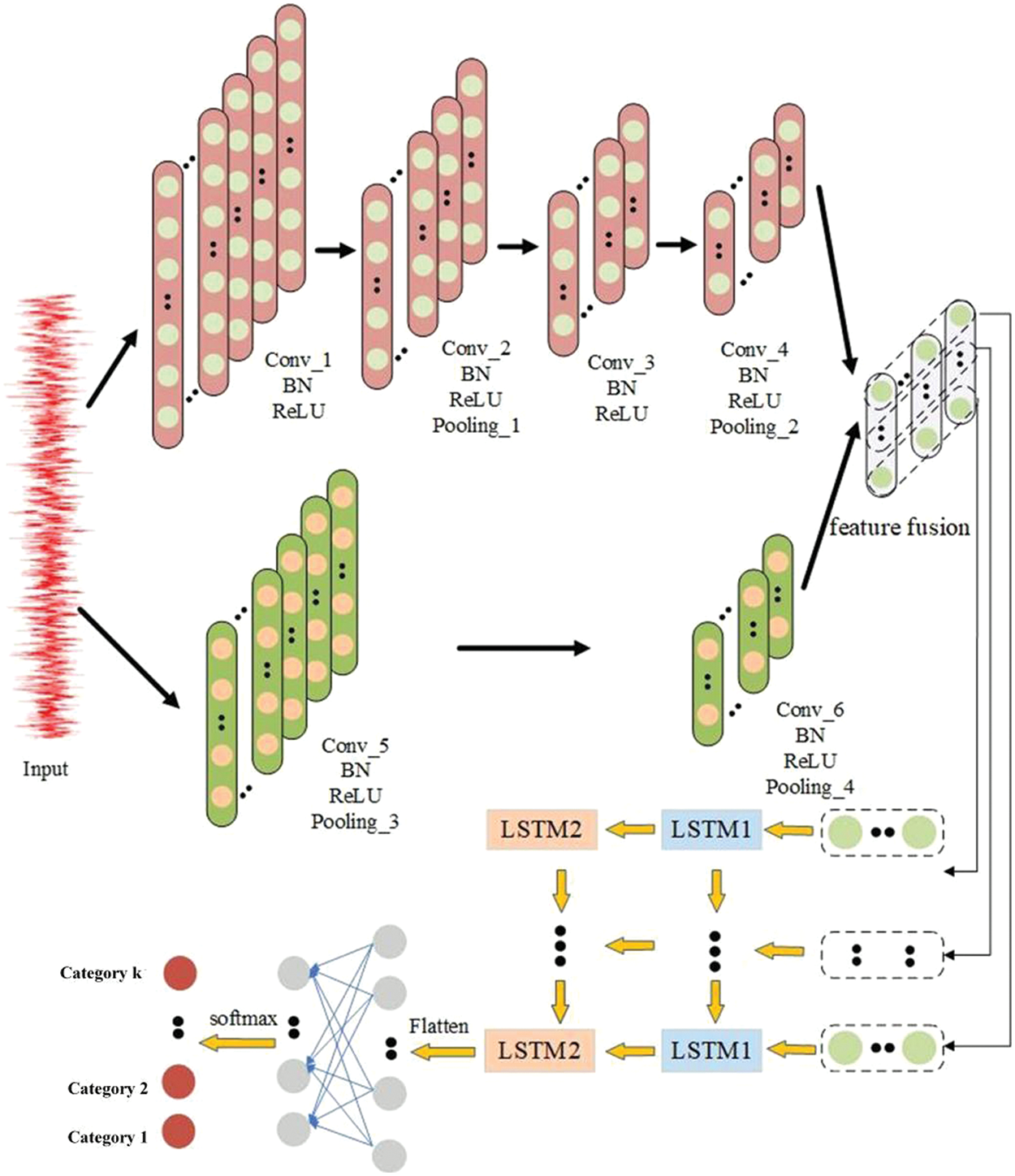
Figure 2: Framework of MSCNN-LSTM

Specifically, the model has two modules: A classifier and a feature extractor. The feature extractor consists of a two-layer LSTM network and a convolutional network made up of two parallel big convolutional kernels and a tiny convolutional kernel. First, both CNNs get the normalized Z-score vibration signal simultaneously. In the lower branch, CNN1, Conv_5, and Conv_6 mine low-frequency data using a 20 * 1 big convolutional kernel. 6 * 1 tiny convolutional kernels are used in the CNN2 upper branch Conv_ 1 to Conv_ All 4 to mine high-frequency data. Second, the element product is utilized to fuse the outputs from the two branches. To further investigate the data that the convolutional network overlooked, the fused features are then input into a two-layer LSTM network. Fig. 2 illustrates how LSTM2 receives input from the hidden state of LSTM1, and how a fully connected layer receives the LTSM2 output for classification. The preceding step’s output influences the subsequent step’s production in LSTM networks. As a result, LSTM networks extract the internal elements of vibration signals and fully use the time series characteristics. Ultimately, the diagnostic outcome is the defect that corresponds to the maximum probability label after the SoftMax function transforms the fully connected layer neurons’ output into the probability distribution of bearing health status.

It is important to note that to increase the model’s learning rate and prevent overfitting, this article adds a BN layer to CNN. As feature extractors, MSCNN and LSTM offer the following benefits: They can automatically learn the features of various vibration signals; CNN employs a shared weight strategy, which drastically lowers the number of parameters and high-dimensional input vectors; the size of the convolutional kernel limits both the input and output of the previous layer; LSTM fully utilizes the global features of vibration signals and improves model generalization.

The parameter list of MSCNN-LSTM is shown in Table 1, and the network containing the LSTM layer is trained using the Adam algorithm. A network with only convolutional layers and no LSTM layers is trained using SGD. During the training process of all models, the learning rate is adjusted in stages, with a total of 200 iterations. The learning rate for the first 60 iterations is set to 0.01, and after 60 iterations, the learning rate is adjusted to 0.001. The batch size is set to 64 throughout the entire training process.

3.2 Network Optimization Learning

Cross entropy is typically used to compute the error between predicted values and true values in multiclass fault diagnosis activities. As a result, the objective function in this article is likewise constructed using it, and the expression is as follows:

ℒ=−1n∑i(yiln⁡softmax(zi))softmax(zi)=exp⁡(zi)∑iKexp⁡(zi)(9)

In the original diagnostic signal formula, yi represents the true value, and zi represents the output of the i−th neuron in the last fully connected layer; softmax(zi) is the probability output of the i−th neuron after passing through the Softmax classifier; n represents the number of training samples; K represents the number of categories.

The original diagnostic signal should be normalized before being fed into two parallel convolutional networks to extract vibration features and gather local spatial correlation features using complementary convolutional kernels of varying widths.

To make up for convolutional networks’ inadequate capacity for global feature capture, the data features are fused using element product fusion and used as feature inputs for the LSTM layer. Temporal features are then recovered utilizing the memory module of hidden units in LSTM. Update the model’s parameters, minimize the cross-entropy objective function, and use error backpropagation. Until the model converges, repeat the first three sections.

Following the MSCNN-LSTM model’s training, test samples will be fed into the model for validation and a diagnostic model will be implemented for fault classification.

4  Experiment

4.1 CWRU Bearing Dataset

The dataset is the CWRU dataset from the Bearing Data Center of Case Western Reserve University [29]. The test bearing works under four working conditions (A0:1797 r/min/0 hp, A1:1772 r/min/hp, A2:1750 r/min/2 hp, A3:1730 r/min/3 hp), so twelve transfer scenarios can be established. As illustrated in Fig. 3, drive end-bearing vibration data with a 12 kHz sampling frequency is adopted in this paper. There are four kinds of health modes, including normal condition (NC), inner ring damage (IF), outer ring damage (OF), and roller damage (RF), and each failure mode has three different severity levels, namely 7, 14 and 21 mils (1 mil = 0.001 in). Therefore, the dataset can form 10 categories (NC, IF-07, IF-14, IF-21, OF-07, OF-14, OF-21, RF-07, RF-14, RF-21). In experiments, there are 500 samples in each category, and each sample is composed of 1024 points. As shown in Table 2, the proportion of training and testing samples is 7:3.

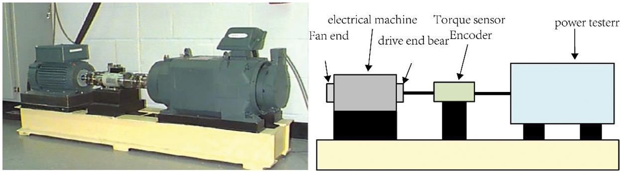
Figure 3: The test rig of CWRU

4.2 Implementation Details and Comparison Approaches

To verify the performance of the proposed method MSCNN-LSTM, the following model was designed for comparative experiments:

CNN1. The most representative deep model is CNN. We use it as a standard for comparison as a result. The portion of MSCNN-LSTM that remains after the LSTM is removed is the network structure. As the initial comparative experiment, we employ convolutional layers 1 through 4 to directly output the results. CNN2. After the LSTM is removed, the network structure is what’s left of MSCNN-LSTM. As the second comparative experiment, we directly output the results using convolutional layers 5 through 6.

CNN1-LSTM. A better recurrent neural network, the long-term dependence of RNN, and the vanishing gradient in real-world applications are issues that can be resolved by the LSTM, increasing the network’s dependability. To extend the duration of the short-term memory, LSTM employs memory blocks to store data selectively. The network structure is what’s left over when CNN2 is removed from MSCNN-LSTM. As the third comparative experiment, we employ convolutional layers 1 through 4 to directly output the findings. CNN2-LSTM. The network structure is what is left over when CNN2 is removed from MSCNN-LSTM. The fourth comparative experiment employs convolutional layers 5 through 6 to directly output the results.

Training time and accuracy can be significantly increased by using Batch Normalization (BN), a technique that standardizes the activation of intermediate layers in deep neural networks. Larger gradient step sizes, faster convergence, and the potential to avoid severe local minima are the outcomes of BN’s continuous correction of the activation output to zero mean and unit standard deviation, which reduces covariate drift. BN also smoothes the optimization environment, which increases the predictability and stability of the gradient behavior and facilitates faster training.

MSCNN-LSTM (w/o BN). The portion of MSCNN-LSTM that remains after the BN is removed is the network structure. As the sixth comparative experiment, we output the results using all convolutional layers. MSCNN-LSTM. We have introduced a BN layer in CNN to improve the learning rate of the model and avoid overfitting. Use the model constructed in the article as the sixth experiment.

4.3 Results of the CWRU Dataset

Table 3 shows the experimental results of CWRU-bearing diagnosis tasks. The accuracy and F1 score of the six methods under four operating conditions A0, A1, A2, and A3 are shown in Table 3, from which the following conclusions can be drawn:

The two CNN1-LSTM indicators have an average increase of 1.5%, although all CNN1 indicators are generally 1.9% greater than CNN2. This suggests that convolutional neural networks with deeper depths produce more abstracted extracted characteristics, which enhances diagnostic performance. Therefore, deepening the network may aid in improving diagnostic outcomes.

When compared to using CNN alone, the reasonable introduction of LSTM based on CNN, the potent feature extraction function of convolutional neural networks, and the good temporal modeling ability of LSTM combined can improve the fault performance of the network. All indicators of CNN1-LSTM and CNN2-LSTM are more than 3.5% higher than CNN1 and CNN2 on average. In comparison to CNN1-LSTM and CNN2-LSTM, the fault diagnostic results of MSCNN-LSTM are 1.7% and 3.5% higher on average. This suggests that learning multi-scale fault features in parallel using a layered structure with multiple pairs of convolutional and pooling layers can significantly improve feature learning ability and enhance fault diagnosis effectiveness. It is clear from the diagnostic results of MSCNN-LSTM that adding BN layers to convolutional networks can improve the network’s ability to represent and extract features. The results are more than 1% higher than the average of MSCNN-LSTM (w/o BN).

In conclusion, MSCNN-LSTM outperforms the other five approaches in terms of accuracy and F1 score, suggesting that the suggested algorithm can complete bearing fault classification tasks in the presence of constant operating conditions.

This article assesses convergence performance using the training process loss as well as the training and testing sets’ accuracy change curves. The training loss and accuracy curves for six distinct approaches under operating condition A0 are displayed in Fig. 4. The horizontal axis represents the number of iterations, the comparative experiment method is inferior to the one suggested in this article among the six comparison methods.

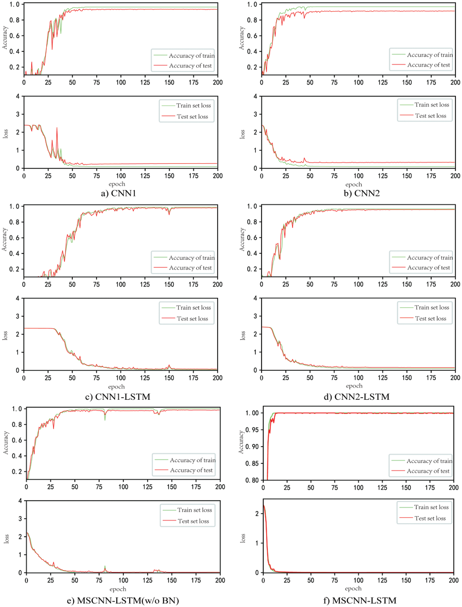
Figure 4: The curve of loss and accuracy changes during training and testing

The superior performance of CNN1-LSTM and CNN2-LSTM models over CNN1 and CNN2 models suggests that adding LSTM layers can significantly increase the accuracy of fault identification. MSCNN-LSTM is better than CNN1-LSTM and CNN2-LSTM. The high convergence speed and accuracy of the LSTM model indicate that parallel multi-scale convolution can learn more fine-grained distinguishable features, which is helpful for fault recognition.

The MSCNN-LSTM (w/o BN) without a BN layer converges after 40 iterations. MSCNN-LSTM only needs 15 iterations to converge, and the convergence curve is smooth. The accuracy of the test set is also quite high, indicating that the BN layer can indeed accelerate model convergence and improve diagnostic accuracy.

By feeding the test samples into the trained MSCNN-LSTM rolling bearing fault detection model, the results were displayed in a confusion matrix, which allowed for a more thorough assessment of the model’s generalization capacity based on the structural characteristics of MSCNN-LSTM. The type of diagnosed rolling bearing defect is represented by the horizontal axis data, whereas the vertical axis data depicts the actual type of rolling bearing failure. The normal recognition rate of the bearing is 100%, as illustrated in Fig. 5, while the rolling element damage recognition rate is comparatively high at 99%. The rolling bearing fault diagnosis model based on the enhanced convolutional neural network long short-term memory network has strong generalization capacity, as evidenced by the average accuracy of 98% for the four types of rolling bearing failures.

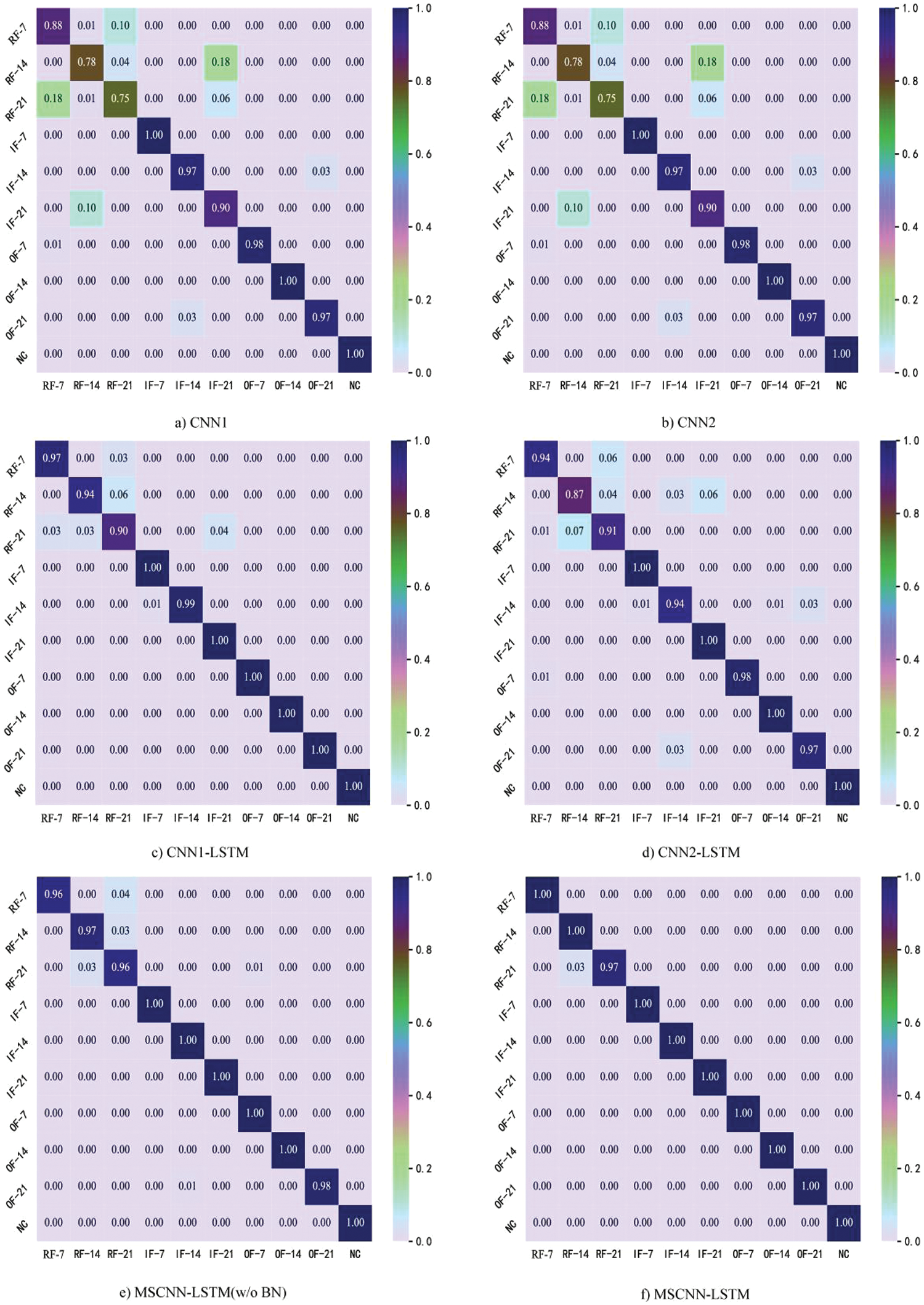
Figure 5: Confusion matrix of four domain adaptation methods

The learned characteristics of CNN1, CNN2, CNN1-LSTM, CNN2-LSTM, MSCNN-LSTM (w/o BN), and MSCNN-LSTM are visualized using t-SNE technology to further demonstrate the performance of the MSCNN-LSTM. As seen in Fig. 6, where various colors stand for various categories of data. It is evident that MSCNN-LSTM successfully distinguishes between distinct health models in addition to precisely identifying diverse sectors. In contrast, features within the same health mode are found to be clustered in other comparison approaches; however, source and target features do not exhibit good alignment within the relevant category. These findings generally provide intuitive evidence that the MSCNN-LSTM can provide superior feature representation and classification performance.

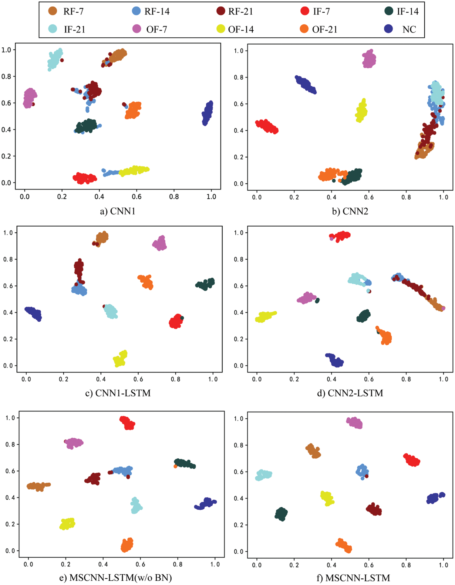
Figure 6: Visualization of learned features on CWRU

4.4 Results of the CWRU Dataset

To verify the universality of the model in diagnosing faults of different types of rolling bearings, this paper introduces bearing fault data collected by Jiangnan University [30]. The data collection frequency is 50 kHz, and it operates at three speeds: 600, 800, and 1000 r/min. The data in this article is categorized into four states: Rolling element failure (RF), inner ring failure (IF), outer ring failure (OF), and normal condition (NC). In the test, there are 500 samples in each category, and each sample is composed of 1024 points. The proportion of training testing samples is 7:3, additionally, the data were split into three datasets: B0, B1, and B2, based on the rotational rates of 600, 800, and 1000 revolutions per minute. Table 4 displays the datasets’ specifics.

On datasets B0, B1, and B2, comparative tests were carried out at various speeds. A comparison was made between the model structure of this experiment and the CWRU bearing dataset. Table 5 displays the experimental outcomes. This shows that, for this experimental dataset, all models’ diagnostic accuracy has dropped. This could be because of the environment and data collection device’s restricted precision. In comparison with models like BiLSTM, 1DCNN, and CNN-LSTM, our model performs better on the B0, B1, and B2 datasets than other approaches, demonstrating its stronger universality and high fault diagnosis performance for various bearing types.

5  Conclusions

The MSCNN-LSTM model’s structure, as well as the steps involved in training and testing, are suggested in this article. Afterward, the CWRU bearing dataset was used to thoroughly validate the MSCNN-LSTM network’s resilience, fault recognition accuracy, and feature extraction capability. The main experimental findings are presented in this article to investigate the internal workings of the model. Real-time bearing status identification is made possible by the technology described in this article, which features a compact network topology and normalized raw data input. It can reliably identify ten distinct fault kinds without requiring any preprocessing and automatically extract features from the raw signal.

According to the experimental results, the combined model performs better under constant operating conditions than some intelligent defect diagnosis systems with a single structure. In addition, the model in this study may reach lower loss values and higher accuracy after fewer iterations, and its convergence pace is steady and quick. Nevertheless, this paper only validates the model’s capacity to diagnose faults under fixed loads; more investigation is required to determine its ability to diagnose problems under fluctuating loads and its anti-noise performance in noisy situations.

There are certain issues with the paper that need to be fixed because of this paper restricted skill set and the circumstances of the experiment. In the future, it will be important to focus on developing a model that can automatically optimize parameters, as the configuration and selection of deep learning parameters rely too heavily on experience. The dataset used in the article was collected in a lab and will eventually be used in real wind farms.

Acknowledgement: In this article, thank you very much to H. C. Zhu and J. Lei. Firstly, I would like to express my gratitude to H. C. Zhu for leading me into the field of fault diagnosis and teaching me how to run programs to adapt to the field of deep learning more quickly. He provided me with ideas in the article. Secondly, I would like to express my gratitude to J. Lei for his assistance in drawing images. Lastly, I would like to thank the reviewers for their feedback, which allowed me to publish my paper faster. Sincere thanks to you all.

Funding Statement: The authors received no specific funding for this study.

Author Contributions: The authors confirm contribution to the paper as follows: Study conception and design: C. M. Wu, S. P. Zheng; data collection: C. M. Wu; analysis and interpretation of results: C. M. Wu, S. P. Zheng; draft manuscript preparation: S. P. Zheng. All authors reviewed the results and approved the final version of the manuscript.

Availability of Data and Materials: The data that support the findings of this study are openly available at http://groups.uni-paderborn.de/kat/BearingDataCenter/.

Conflicts of Interest: The authors declare that they have no conflicts of interest to report regarding the present study.

References

1. J. C. Yin, M. Q. Xu, and H. L. Zheng, “Fault diagnosis of bearing based on symbolic aggregate approximation and Lempel-Ziv,” Measurement, vol. 138, no. 4, pp. 206–216, May 2019. doi: 10.1016/j.measurement.2019.02.011. [Google Scholar] [CrossRef]

2. L. Zhang and N. Q. Hu, “Fault diagnosis of sun gear based on continuous vibration separation and minimum entropy deconvolution,” Measurement, vol. 141, pp. 332–344, Jul. 2019. doi: 10.1016/j.measurement.2019.04.049. [Google Scholar] [CrossRef]

3. Y. Liu, J. Wang, and Y. Shen, “Research on verification of sensor fault diagnosis based on BP neural network,” in 2020 11th Int. Conf. Progn. Syst. Health Manag. (PHM-2020 Jinan), Jinan, China, 2020, pp. 456–460. [Google Scholar]

4. Q. L. Hou, Y. Liu, P. P. Guo, C. T. Shao, L. Cao and L. Huang, “Rolling bearing fault diagnosis utilizing pearson’s correlation coefficient optimizing variational mode decomposition based deep learning model,” in 2022 IEEE Int. Conf. Sensing, Diagn., Progn., Control (SDPC), Chongqing, China, Aug. 2022, pp. 206–213. [Google Scholar]

5. H. D. Shao, H. K. Jiang, H. W. Zhao, and F. A. Wang, “A novel deep autoencoder feature learning method for rotating machinery fault diagnosis,” Mech. Syst. Signal. Process., vol. 195, no. 8, pp. 187–204, Oct. 2017. doi: 10.1016/j.ymssp.2017.03.034. [Google Scholar] [CrossRef]

6. J. Q. Zhang, S. Yi, L. Guo, H. L. Gao, X. Hong and H. L. Song, “A new bearing fault diagnosis method based on modified convolutional neural networks,” Chin. J. Aeronaut., vol. 33, no. 2, pp. 439–447, Feb. 2020. doi: 10.1016/j.cja.2019.07.011. [Google Scholar] [CrossRef]

7. H. M. Ahmad and A. Rahimi, “Deep learning methods for object detection in smart manufacturing: A survey,” J. Manuf. Syst., vol. 64, no. 1, pp. 181–196, Jul. 2022. doi: 10.1016/j.jmsy.2022.06.011. [Google Scholar] [CrossRef]

8. C. Y. Chen, A. Seff, A. Kornhauser, and J. X. Xiao, “DeepDriving: Learning affordance for direct perception in autonomous driving,” in 2015 IEEE Int. Conf. Comput. Vis. (ICCV), Santiago, Chile, 2015, pp. 2722–2730. [Google Scholar]

9. Q. Rao and J. Frtunikj, “Deep learning for self-driving cars: Chances and challenges,” in 2018 IEEE/ACM 1st International Workshop on Software Engineering for AI in Autonomous Systems (SEFAIAS), Gothenburg, Sweden, 2018, pp. 35–38. [Google Scholar]

10. G. Singh, P. Pidadi, and D. S. Malwad, “A review on applications of computer vision,” Lect. Notes Netw. Syst., vol. 647, pp. 464–479, 2023. doi: 10.1007/978-3-031-27409-1_42. [Google Scholar] [CrossRef]

11. F. Alsakka, S. Assaf, I. El-Chami, and M. Al-Hussein, “Computer vision applications in offsite construction,” Autom. Constr., vol. 154, Oct. 2023. doi: 10.1016/j.autcon.2023.104980. [Google Scholar] [CrossRef]

12. H. Y. Ma, D. Zhou, Y. J. Wei, W. Wu, and E. Pan, “Intelligent bearing fault diagnosis based on adaptive deep belief network under variable working conditions,” (in ChineseJ. Shanghai Jiaotong Univ., vol. 56, no. 10, pp. 1368–1378, 2022. doi: 10.16183/j.cnki.jsjtu.2021.161. [Google Scholar] [CrossRef]

13. Z. Meng, X. Y. Zhan, J. Li, and Z. Z. Pan, “An enhancement denoising autoencoder for rolling bearing fault diagnosis,” Measurement, vol. 130, pp. 448–454, Aug. 2018. doi: 10.1016/j.measurement.2018.08.010. [Google Scholar] [CrossRef]

14. R. Y. Du, F. L. Liu, L. J. Zhang, Y. H. Ji, J. L. Xu and F. Gao, “Modulation recognition based on denoising bidirectional recurrent neural network,” Wirel. Pers. Commun., vol. 132, no. 4, pp. 2437–2455, 2023. doi: 10.1007/s11277-023-10725-5. [Google Scholar] [CrossRef]

15. D. Pallavi and T. P. Anithaashri, “Novel predictive analyzer for the intrusion detection in student interactive systems using convolutional neural network algorithm over artificial neural network algorithm,” in Proc. 2022 4th Int. Conf. Adv. Computing, Commun. Control Netw., Greater Noida, India, 2022, pp. 638–641. [Google Scholar]

16. Y. G. Yang, H. B. Shi, Y. Tao, Y. Ma, B. Song and S. Tan, “A semi-supervised feature contrast convolutional neural network for processes fault diagnosis,” J. Taiwan Inst. Chem. Eng., vol. 151, Oct. 2023. doi: 10.1016/j.jtice.2023.105098. [Google Scholar] [CrossRef]

17. B. Y. Zhang, X. Y. Yan, G. Y. Liu, and K. X. Fan, “Multi-source fault diagnosis of chiller plant sensors based on an improved ensemble empirical mode decomposition Gaussian mixture model,” Energy Rep., vol. 8, pp. 2831–2842, Nov. 2022. doi: 10.1016/j.egyr.2022.01.179. [Google Scholar] [CrossRef]

18. Y. X. Chen, A. Zhu, and Q. S. Zhao, “Rolling bearing fault diagnosis based on flock optimization support vector machine,” in IEEE 7th Inf. Technol. Mechatron. Eng. Conf., Chongqing, China, 2023, pp. 1700–1703. doi: 10.1109/ITOEC57671.2023.10292080. [Google Scholar] [CrossRef]

19. P. P. Han, C. B. He, S. L. Lu, Y. B. Liu, and F. Liu, “Rolling bearing fault diagnosis based on variational mode decomposition and cyclostationary analysis,” in 2021 Int. Conf. Sensing, Meas. Data Anal. Era Artif. Intell. (ICSMD), Nanjing, China, 2021, pp. 1–6. doi: 10.1109/ICSMD53520.2021.9670846. [Google Scholar] [CrossRef]

20. D. K. Soother, I. H. Kalwar, T. Hussain, B. S. Chowdhry, S. M. Ujjan and T. D. Memon, “A novel method based on UNET for bearing fault diagnosis,” Comput. Mater. Contin., vol. 69, no. 1, pp. 393–408, 2021. doi: 10.32604/cmc.2021.014941. [Google Scholar] [CrossRef]

21. L. T. Gao, X. M. Wang, T. Wang, and M. Y. Chang, “WDBM: Weighted deep forest model based bearing fault diagnosis method,” Comput. Mater. Contin., vol. 72, no. 3, pp. 4742–4754, 2022. doi: 10.32604/cmc.2022.027204. [Google Scholar] [CrossRef]

22. B. Yang, Y. G. Lei, F. Jia, and S. B. Xing, “An intelligent fault diagnosis approach based on transfer learning from laboratory bearings to locomotive bearings,” Mech. Syst. Signal. Process., vol. 122, pp. 692–706, May 2019. doi: 10.1016/j.ymssp.2018.12.051. [Google Scholar] [CrossRef]

23. Y. G. Lei, B. Yang, X. W. Jiang, F. Jia, N. P. Li and A. K. Nandi, “Applications of machine learning to machine fault diagnosis: A review and roadmap,” Mech. Syst. Signal. Process., vol. 138, pp. 106587, Apr. 2020. doi: 10.1016/j.ymssp.2019.106587. [Google Scholar] [CrossRef]

24. W. N. Lu, B. Liang, Y. Cheng, D. S. Meng, J. Yang and T. Zhang, “Deep model-based domain adaptation for fault diagnosis,” IEEE Trans. Ind. Electron., vol. 64, no. 3, pp. 2296–2305, Mar. 2017. doi: 10.1109/TIE.2016.2627020. [Google Scholar] [CrossRef]

25. X. Li, W. Zhang, Q. Ding, and J. Q. Sun, “Multi-Layer domain adaptation method for rolling bearing fault diagnosis,” Signal Process., vol. 157, pp. 180–197, Apr. 2019. doi: 10.1016/j.sigpro.2018.12.005. [Google Scholar] [CrossRef]

26. N. Takahashi, N. Goswami, and Y. Mitsufuji, “Mmdenselstm: An efficient combination of convolutional and recurrent neural networks for audio source separation,” in 16th Int. Workshop Acoustic Signal Enhanc., Tokyo, Japan, Nov. 2018, pp. 106–110. [Google Scholar]

27. A. T. Mwelinde, Z. Y. Han, H. Y. Jin, T. Abayo, and H. Y. Fu, “Bearing fault diagnosis integrated model based on hierarchical fuzzy entropy, convolutional neural network and long short-term memory,” in 2022 Int. Conf. Sensing, Meas. Data Anal. Era Artif. Intell. (ICSMD), Harbin, China, 2022, pp. 1–5. [Google Scholar]

28. X. H. Liao and Y. H. Mao, “Rolling bearing fault diagnosis method based on attention mechanism and CNN-BiLSTM,” in Proc. SPIE—Int. Soc. Opt. Eng., Hangzhou, China, Jul. 2023, pp. 3377–3410. [Google Scholar]

29. W. A. Smith and R. B. Randall, “Rolling element bearing diagnostics using the case western reserve university data: A benchmark study,” Mech. Syst. Signal. Process., vol. 64–65, pp. 100–131, Dec. 2015. doi: 10.1016/j.ymssp.2015.04.021. [Google Scholar] [CrossRef]

30. Z. Q. Chen, S. C. Deng, X. D. Chen, C. Li, R. Sanchez and H. F. Qin, “Deep neural networks-based rolling bearing fault diagnosis,” Microelectron. Reliab., vol. 75, pp. 327–333, Aug. 2017. doi: 10.1016/j.microrel.2017.03.006. [Google Scholar] [CrossRef]